Generation of Polynomial Automorphisms Appropriate for the Generalization of Fuzzy Connectives

Abstract

Fuzzy logic is becoming one of the most-influential fields of modern mathematics with applications that impact not only other sciences, but society in general. This newly found interest in fuzzy logic is in part due to the crucial role it plays in the development of artificial intelligence. As a result, new tools and practices for the development of the above-mentioned field are in high demand. This is one of the issues this paper was composed to address. To be more specific, a sizable part of fuzzy logic is the study of fuzzy connectives. However, the current method used to generalize them is restricted to the use of basic automorphisms, which hinders the creation of new fuzzy connectives. For this reason, in this paper, a new method of generalization is conceived of that aims to generalize the fuzzy connectives using polynomial automorphism functions instead. The creation of these automorphisms is achieved through numerical analysis, an endeavor that is supported with programming applications that, using mathematical modeling, validate and visualize the research. Furthermore, the automorphisms satisfy all the necessary criteria that have been established for use in the generalization process and, consequently, are used to successfully generalize fuzzy connectives. The result of the new generalization method is the creation of new usable and flexible fuzzy connectives, which is very promising for the future development of the field.

1. Introduction

The main focus of this paper is the production of polynomial automorphisms, which are able to be used to generalize fuzzy connectives. Achieving this is important because of the crucial role that fuzzy connectives play in the fields of fuzzy logic and, consequently, artificial intelligence [1]. To be more specific, the above-mentioned fields will benefit from advancements in the study of fuzzy connectives, like the one presented in this paper, as they make possible further developments and optimizations. In order to further understand the significance of fuzzy connectives, the following paragraphs present the history of the field through the most-notable published research.

The study of fuzzy connectives started with the publication of the paper “Statistical metrics” by Menger [2], which used the concept of t-norms for the first time. Then, the field progressed with the work of Schweizer B.and Sklar A. [3] which spanned several years. Specifically, publications in 1958, 1960, 1961, and 1983 defined the theorems of ordinary rules and documented their findings. The work of Schweizer B. and Sklar A. was built upon by Ling C.H. [4], who, in 1965, determined the Archimedean t-norms. In 1979, Frank M.J. [5] expanded upon the previous research by defining the parameterized families of t-norms. However, the progress did not stop, as Navara M. [6] in 1999, Gottwald S. [7] in 2000, and Klement E.P. [8] in 2001 proposed the strategy of generating t-norms via automorphism and additive generative functions. Modus ponens and tollens were discovered in 2004 by Kerre E. et al. [9]. In the same year, Kerre E. and Nachtegael M. [10] defined the fuzzy mathematical morphology. Four years later, in 2008, the implications of various properties were found by Trillas E. et al. [11].

However, previously, in 2006, Bustince H. et al. [12] published a work on fuzzy measures and image processing. Thereafter, Baczyński M. and Jayaram B., as well as Mas M. et al. [13,14], in 2007, crafted a method that generates (S,N)-implications. A strategy for creating R-implications was invented by Fodor J.C. and Roubens M. [15], in 1994. The generation of QL- and D-operations constituted the main objective of the process published by Mas M. et al. [16] in 2006. In 2004, the problem of generating f- and g-implications was tackled by Yager R.R. [17]. Finally, in 2012, Callejas C. et al. [18] proposed a method that creates any fuzzy implication.

For a decade, from 2012 to 2021, there was little to no further research about the subject of fuzzy connectives. Nonetheless, in 2022, Makariadis S. and Papadopoulos B. [19] published the paper titled “Generalization of Fuzzy Connectives”, which brought the focus back to the field. This new development motivated the creation of this paper as a proof that the interest brought to the field by the 2022 paper was not temporary, but rather, the beginning to a series of new discoveries. So, the main goal of this work is to prove that the study of fuzzy connectives is not complete by developing a new method of generalizing fuzzy connectives. The conclusions drawn from the research presented in this paper are multiple. To be more specific, the field of the generalization of fuzzy connectives is proven to be still active, evidenced by the creation of a new method of generalizing fuzzy connectives that provides more flexibility and usability in comparison with established methods. Furthermore, it was concluded that other fields can be used in combination with fuzzy logic to create new tools and, finally, that automation paired with fuzzy logic can offer significant time savings gains. Finally, it is important to mention that the structure of the paper is as follows:

Introduction: In this section, a brief presentation of the research included in this paper takes place. Furthermore, the history, as well as the state of the paper’s field are explored.

Preliminaries: In this section, the main concepts necessary for the understanding of the paper are defined.

Materials and Methods: In this section, the methods and strategies followed in the paper are explained in detail before being mathematically proven.

Results: In this section, the results of the paper are presented.

Discussion: In this section, the results of the paper are discussed and interpreted from the perspective of previous studies.

Conclusions: In this section, the conclusions drawn from the whole paper are presented.

2. Preliminaries

This section is dedicated to the display of the basic concepts used throughout the paper. To be more specific, the main points of interest are fuzzy negations, triangular norms (conjunctions and disjunctions), and fuzzy implications, as they form the basis of fuzzy connectives. Furthermore, emphasis is given to the explanation of notions such as automorphisms and Lagrange interpolation.

2.1. Fuzzy Negations

The definition displayed in this subsection can be found in the following references: Baczyński M., 1.4.1–1.4.2 Definitions, pp. 13–14, [20], Bedregal B.C., p. 1126, [21], Fodor J., 1.1–1.2 Definitions, p. 3, [15], Gottwald S., 5.2.1 Definition, p. 85, [7], Weber S., 3.1 Definition, p. 121, [22], and Trillas E., p. 49, [23].

Definition 1. 

A function $N:(0,1)\to [0,1]$ is called a fuzzy negation if

• $\left(N1\right)N\left(0\right)=1,N\left(1\right)=0;$
• $\left(N2\right)Nisdecreasing.$
  A fuzzy negation N is called strict if, in addition to the former properties, the following apply:
• (N3) N is strictly decreasing;
• (N4) N is continuous.
  A fuzzy negation N is called strong if the following property is satisfied:
• $\left(N5\right)N\left(N\right(x\left)\right)=x,x\in [0,1].$

2.2. Triangular Norms (Conjunctions)

In this subsection, the definition and properties of t-norms will be provided.

The sequent definition can be found in: Klement E.P et al., 1.1 Definition, pp. 4–10, [8], Baczyński M., 2.1.1, 2.1.2 Definitions, pp. 41–42, [20], Weber S., 2.1 Definition, pp. 116–117, [22], and Yun s., p. 16, [24].

Definition 2. 

A function $T:{[0,1]}^2\to [0,1]$ is called a triangular norm, or t-norm, if it satisfies, for all $x,y\in [0,1]$, the following conditions:

$\left(T1\right)T(x,y)=T(y,x),\left(commutativity\right);$

$\left(T2\right)T(x,T(y,z\left)\right)=T\left(T\right(x,y),z),\left(associativity\right);$

$\left(T3\right)ify\le z,thenT(x,y)\le T(x,z),\left(monotonicity\right);$

$\left(T4\right)T(x,1)=x,\left(boundarycondition\right).$

2.3. Triangular Conorms (Disjunctions)

S-conorms allow for the generalization of the union in a lattice or disjunction in logic. The sequent definition can be found in: Klement E.P et al., 1.13 Definition, p. 11, [8], Baczyński M., 2.2.1, 2.2.2 Definitions, pp. 45–46, [20], and Yun s., p. 22, [24].

Definition 3. 

A function $S:{[0,1]}^2\to [0,1]$ is called a triangular conorm (t-conorm) if it satisfies, for all $x,y\in [0,1]$, the following conditions:

$\begin{array}{c}\left(S1\right):S\left(x,y\right)=S\left(y,x\right)\left(commutativity\right);\hfill \\ \left(S2\right):S\left(x,S\left(y,z\right)\right)=S\left(S\left(x,y\right),z\right)\left(associativity\right);\hfill \\ \left(S3\right):\mathrm{If}y\le z,\mathrm{then}S\left(x,y\right)\le S\left(x,z\right)\left(monotonicity\right);\hfill \\ \left(S4\right):S\left(x,0\right)=x(\mathrm{neutral}\mathrm{element}0).\hfill \end{array}$

2.4. Fuzzy Implications

Fuzzy implications play a crucial role in fuzzy logic as they represent what the classical implications are in crisp logic. The primary use of fuzzy implication functions is the execution of any fuzzy “if–then” rule on fuzzy systems.

The sequent definition can be found: Baczyński M., p. 2, [20], Yun s., p. 5, [24], and Fodor J., p. 299, [25].

Definition 4. 

A binary operator $I:{[0,1]}^2\to [0,1]$ is said to be an implication function, or an implication, if, for all $x,y\in [0,1]$, it satisfies:

$\begin{array}{c}\left(I1\right):I\left(x,z\right)\ge I\left(y,z\right)whenx\le y,isinthefirstplace\left(antitonicity\right);\hfill \\ \left(I2\right):I\left(x,y\right)\le I\left(x,z\right)wheny\le z,isinthesecondplace\left(isotonicity\right);\hfill \\ \left(I3\right):I\left(0,0\right)=1,\left(boundarycondition\right);\hfill \\ \left(I4\right):I\left(1,1\right)=1,\left(boundarycondition\right);\hfill \\ \left(I5\right):I\left(1,0\right)=0,\left(boundarycondition\right).\hfill \end{array}$

A function $I:{[0,1]}^2\to [0,1]$ is called a fuzzy implication only if it satisfies $\left(I1\right)$–$\left(I5\right)$.

2.5. Automorphism Functions

Automorphisms are necessary for the generalization of fuzzy connectives, and as a result, they shape, to a degree, how the field evolves.

The sequent definition can be found in: Bedregal B., p. 1127, [21], and Yun s., p. 13, [24].

Definition 5. 

A mapping $\phi :[\mathrm{a},\mathrm{b}]\to [\mathrm{a},\mathrm{b}]\left(\right[\mathrm{a},\mathrm{b}]\subset \mathbb{R})$ is an automorphism of the interval [a, b] if it is continuous and strictly increasing and satisfies the boundary conditions: $\phi \left(a\right)=a$ and $\phi \left(b\right)=b$. If φ is an automorphism of the unit interval, then ${\phi }^{-1}$ is also an automorphism of the unit interval.

2.6. Lagrange Interpolating Polynomial

The following definition was retrieved from [26].

Definition 6. 

The Lagrange interpolating polynomial is the polynomial $P\left(x\right)$ of degree $\le (n-1)$ that passes through the n points $\left(x_1,y_1=f\left(x_1\right)\right)$, $\left(x_2,y_2=f\left(x_2\right)\right),\dots ,\left(x_n,y_n=f\left(x_n\right)\right)$, and is given by

$$P\left(x\right)=\sum _{j=1}^n{P}_j\left(x\right),$$

where

$$P_j\left(x\right)=y_j\prod _{\begin{array}{c}k=1\\ k\ne j\end{array}}^n\frac{x-x_k}{x_j-x_k}.$$

Written explicitly,

$P\left(x\right)=\frac{\left(x-x_2\right)\left(x-x_3\right)\cdots \left(x-x_n\right)}{\left(x_1-x_2\right)\left(x_1-x_3\right)\cdots \left(x_1-x_n\right)}{y}_1+\frac{\left(x-x_1\right)\left(x-x_3\right)\cdots \left(x-x_n\right)}{\left(x_2-x_1\right)\left(x_2-x_3\right)\cdots \left(x_2-x_n\right)}{y}_2+\cdots +\frac{\left(x-x_1\right)\left(x-x_2\right)\cdots \left(x-x_{n-1}\right)}{\left(x_n-x_1\right)\left(x_n-x_2\right)\cdots \left(x_n-x_{n-1}\right)}{y}_n.$

3. Materials and Methods

As mentioned in the above segments, this paper is focused on the creation of automorphisms that can be used to generalize fuzzy connectives. The generalization of fuzzy connectives using automorphisms was achieved with the use of one of the following equations:

$$N_{\phi }\left(x\right)={\phi }^{-1}\left(N\left(\phi \left(x\right)\right)\right),\forall x\in [0,1]$$

(1)

$$T_{\phi }(x,y)={\phi }^{-1}\left(T(\phi \left(x\right),\phi \left(y\right))\right),\forall x,y\in [0,1]$$

(2)

$$S_{\phi }(x,y)={\phi }^{-1}\left(S(\phi \left(x\right),\phi \left(y\right))\right),\forall x,y\in [0,1]$$

(3)

$$I_{\phi }(x,y)={\phi }^{-1}\left(I(\phi \left(x\right),\phi \left(y\right))\right),\forall x,y\in [0,1]$$

(4)

The process of generalization, as displayed above, (1)–(4), involves the use of an automorphism and a fuzzy connective. In [19], the approach of using different fuzzy connective families in conjunction with basic automorphisms was used to achieve generalization. This paper, however, explores the prospect of pairing well-known fuzzy connectives with polynomial automorphisms instead of basic ones.

The reason that moved the paper towards this direction is, firstly, that the fuzzy connective part of the equations has already been researched in regard to generalization and, secondly, the fact that the need for new automorphisms cannot be satisfied by the limited number of practical basic automorphisms (Figure 1). To be more specific, it is not a viable solution to expand further than a few degrees of the mentioned automorphisms, as doing so would lead to computationally intensive and complex scenarios. As a result, the need for new practical automorphisms remains unaddressed, and a task is accomplished in this paper by the use of polynomial automorphisms.

However, currently, there are no appropriate automorphisms for use in the generalization of fuzzy connectives. So, before implementing the new strategy, it was necessary to craft a procedure for generating the necessary polynomial automorphisms. The main problem that was encountered by pursuing this endeavor is the fact that it is notoriously difficult to develop new automorphisms, with the task becoming even more complex when fuzzy logic is involved as the new polynomial functions must not only satisfy the automorphism criteria, but also the restrictions of fuzzy logic.

The problem was addressed by the composition of an algorithm that using numerical analysis methods generates the needed polynomial automorphisms. The algorithm is described in Theorem 1:

Theorem 1. 

Three abscissas are chosen from $[0,1]$: $x_0=0,x_1,0<x_1<1,x_2=1$.

Let $f:[0,1]\to [0,1]$ be an automorphism function with the formula: $f\left(\mathrm{x}\right)=x·\sqrt{x}$.

The corresponding ordinates are calculated with f: $f\left(0\right)=0$, $f\left(x_1\right)=x_1·\sqrt{x_1}$, $f\left(1\right)=1$.

The Lagrange interpolation formula:

$$L\left(x\right)=\frac{\left(\left(x-x_1\right)\left(x-x_2\right)\right)f\left(x_0\right)}{\left(x_0-x_1\right)\left(x_0-x_2\right)}+\frac{\left(\left(x-x_0\right)\left(x-x_2\right)\right)f\left(x_1\right)}{\left(x_1-x_0\right)\left(x_1-x_2\right)}+\frac{\left(\left(x-x_0\right)\left(x-x_1\right)\right)f\left(x_2\right)}{\left(x_2-x_0\right)\left(x_2-x_1\right)}$$

(5)

for the generation of second-degree polynomials is used.

The result is the generation of a second-degree polynomial with the formula:

$$L\left(x\right)=\frac{\sqrt{x_1}-1}{x_1-1}·x^2+\frac{x_1-\sqrt{x_1}}{x_1-1}·x$$

(6)

Let $\phi :[0,1]\to [0,1]$ be a function with the formula: $\phi \left(x\right)=\frac{\sqrt{x_1}-1}{x_1-1}·x^2+\frac{x_1-\sqrt{x_1}}{x_1-1}·x$.

Then, φ is an invertible automorphism function.

As is visible in Theorem 1, the algorithm responsible for the generation of the polynomial automorphisms has multiple steps. However, before explaining them, it was deemed necessary to highlight a key decision that shaped the final result.

The decision mentioned was about the degree of the generated polynomial. To be more specific, in this paper, the generation of second-degree polynomials was pursued because a major focus was given to the production of new automorphisms that can replace the basic ones while bypassing problems like complexity and computational resources, which plague higher degrees. However, it is important to note that, according to the results that the current strategy presents, the generation of higher-degree polynomials appropriate for fuzzy connective generalization is possible. This direction will be further explored in the “Discussion” Section of this paper.

The explanation of Theorem 1 begins with the choice of three abscissas. These values are utilized by the function f, which calculates the corresponding ordinates, leading to the creation of a set of three points. The choice of the function f is crucial to the success of this endeavor because it influences the properties of the produced polynomial. The main point of interest regarding those properties is the fact that the generated polynomials must satisfy the automorphism criteria for use in fuzzy logic. One of the criteria is the fact that the polynomial must cross the points (0,0) and (1,1). The result drawn from this realization is dual. Firstly, two of the three abscissas must be set to 0 and 1, so that the above-mentioned points can be realized. At this point, it is important to mention that the abscissa of the third point is a parameter with a value between 0 and 1 (as this is the interval to which fuzzy logic is applied). Secondly, a function f must be selected so that it can return the appropriate ordinates and complete the creation of the points. The crossing of these two points by the polynomial is guaranteed by the Lagrange interpolation, which produces polynomials that cross all the points that are given as an input and, consequently, crossing (0,0)–(1,1).

When researching functions that would be applicable for this use, the goal was to pinpoint a function that not only satisfied the above limitations, but had a power approximating the degree of the polynomial. In the beginning, the use of the $x^2$ function among other low-degree basic automorphisms was considered. However, the use of these functions was found to be problematic, as for particular values of the third abscissa, the polynomials they generated were basic automorphisms. As a result, the function $x·\sqrt{x}$ was selected for the role of f. This decision was based on the fact that this function has a power that approximately is the nearest to a second-degree polynomial function while providing acceptable and consistent results.

Finally, the points are replaced to the Lagrange interpolation formula for second-degree polynomials, and a general automorphism is generated that includes the third abscissa value as a parameter. Furthermore, the generated automorphism is invertible, and as a result, it can be used for the generalization of fuzzy connectives. The innovative aspect of the automorphism-generation strategy presented in this paper is the fact that every value of the parameter can produce a unique invertible automorphism and, consequently, provide an infinite number of generalized fuzzy connectives. The proof of Theorem 1 is the following:

Proof of Theorem 1. 

Let $f:[0,1]\to [0,1]$ be an automorphism function with the formula: $f\left(\mathrm{x}\right)=x·\sqrt{x}$.

Three abscissas are chosen from $[0,1]$: $x_0=0,x_1,0<x_1<1,x_2=1$.

The corresponding ordinates are calculated with f: $f\left(0\right)=0$, $f\left(x_1\right)=x_1·\sqrt{x_1}$, $f\left(1\right)=1$.

The points generated are replaced in the Lagrange interpolation (5), and the polynomial (6) is constructed:

$\begin{array}{c}L\left(x\right)=\frac{\left(\left(x-x_1\right)\left(x-x_2\right)\right)·f\left(x_0\right)}{\left(x_0-x_1\right)\left(x_0-x_2\right)}+\frac{\left(\left(x-x_0\right)\left(x-x_2\right)\right)·f\left(x_1\right)}{\left(x_1-x_0\right)\left(x_1-x_2\right)}+\frac{\left(\left(x-x_0\right)\left(x-x_1\right)\right)·f\left(x_2\right)}{\left(x_2-x_0\right)\left(x_2-x_1\right)}\iff \\ L\left(x\right)=\frac{\left(\left(x-x_1\right)\left(x-1\right)\right)·f\left(0\right)}{\left(0-x_1\right)\left(0-1\right)}+\frac{\left(\left(x-0\right)\left(x-1\right)\right)·f\left(x_1\right)}{\left(x_1-0\right)\left(x_1-1\right)}+\frac{\left(\left(x-0\right)\left(x-x_1\right)\right)·f\left(1\right)}{\left(1-0\right)\left(1-x_1\right)}\iff \\ L\left(x\right)=\frac{\left(\left(x-x_1\right)\left(x-1\right)\right)·0}{\left(0-x_1\right)\left(0-1\right)}+\frac{\left(\left(x-0\right)\left(x-1\right)\right)·(x_1·\sqrt{x_1})}{\left(x_1-0\right)\left(x_1-1\right)}+\frac{\left(\left(x-0\right)\left(x-x_1\right)\right)·1}{\left(1-0\right)\left(1-x_1\right)}\iff \\ L\left(x\right)=\frac{x\left(x-1\right)·(x_1·\sqrt{x_1})}{x_1·\left(x_1-1\right)}-\frac{x\left(x-x_1\right)}{\left(x_1-1\right)}\iff \\ L\left(x\right)=\frac{\sqrt{x_1}-1}{x_1-1}·x^2+\frac{x_1-\sqrt{x_1}}{x_1-1}·x\end{array}$

Let $\phi :[0,1]\to [0,1]$ be a function with the formula:

$$\phi \left(x\right)=\frac{\sqrt{x_1}-1}{x_1-1}·x^2+\frac{x_1-\sqrt{x_1}}{x_1-1}·x$$

(7)

$\begin{array}{c}\phi \left(0\right)=0\\ \phi \left(1\right)=1\\ {\phi }^{\prime }\left(x\right)=\frac{2·(\sqrt{x_1}-1)}{x_1-1}·x+\frac{x_1-\sqrt{x_1}}{x_1-1}\\ x_1<1\iff x_1-1<0\\ x_1<1\iff \sqrt{x_1}<1\iff \sqrt{x_1}-1<0\\ \frac{2·(\sqrt{x_1}-1)}{x_1-1}>0\\ {\phi }^{\prime }\left(x\right)>0\Rightarrow \phi strictlyincreasing[0,1]\end{array}$

$$\begin{array}{c}\phi \left(x\right)=y\iff \frac{\sqrt{x_1}-1}{x_1-1}·x^2+\frac{x_1-\sqrt{x_1}}{x_1-1}·x=y\iff \frac{\sqrt{x_1}-1}{x_1-1}·x^2+\frac{x_1-\sqrt{x_1}}{x_1-1}·x-y=0\\ D={\left(\frac{x_1-\sqrt{x_1}}{x_1-1}\right)}^2-4·\left(\frac{\sqrt{x_1}-1}{x_1-1}\right)\left(-y\right)\iff \\ D=\frac{{\left(x_1-\sqrt{x_1}\right)}^2+4·y·\left(1-x_1\right)·\left(1-\sqrt{x_1}\right)}{{\left(1-x_1\right)}^2}\\ x=\frac{x_1-\sqrt{x_1}+\sqrt{{\left(x_1-\sqrt{x_1}\right)}^2+4·y·\left(1-x_1\right)·\left(1-\sqrt{x_1}\right)}}{2·\left(1-\sqrt{x_1}\right)}\\ {\phi }^{-1}\left(x\right)=\frac{x_1-\sqrt{x_1}+\sqrt{{\left(x_1-\sqrt{x_1}\right)}^2+4·x·\left(1-x_1\right)·\left(1-\sqrt{x_1}\right)}}{2·\left(1-\sqrt{x_1}\right)}\end{array}$$

where D is the discriminant of the equation $\frac{\sqrt{x_1}-1}{x_1-1}·x^2+\frac{x_1-\sqrt{x_1}}{x_1-1}·x-y=0$.

So, the inverse of $\phi$ is:

$${\phi }^{-1}\left(x\right)=\frac{x_1-\sqrt{x_1}+\sqrt{{\left(x_1-\sqrt{x_1}\right)}^2+4·x·\left(1-x_1\right)·\left(1-\sqrt{x_1}\right)}}{2·\left(1-\sqrt{x_1}\right)}$$

(8)

□

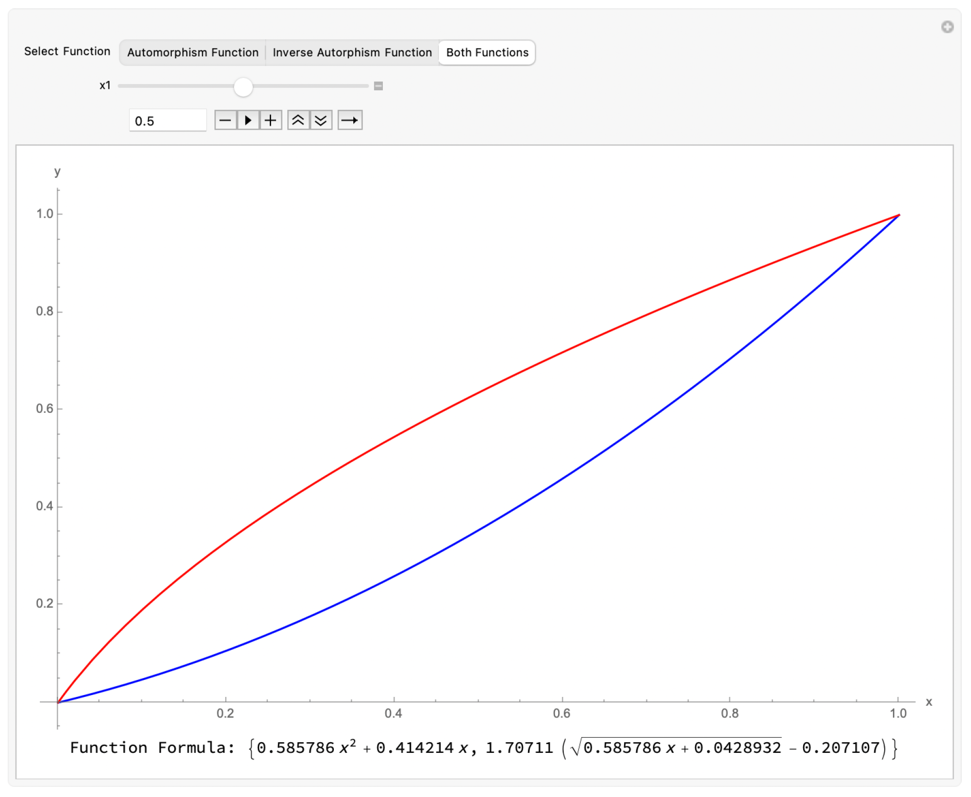
The graph of the generalized automorphism functions $\phi$, ${\phi }^{-1}$ and their symmetry are shown in Figure 2, Figure 3 and Figure 4, when a parameter $x_1=0.5$.

As mentioned at the start of this section, in this paper, the method of using polynomial automorphisms instead of basic ones for the generalization of fuzzy connectives is proposed. So, after proving the polynomial-automorphism-generation strategy, the main problem hindering the implementation of the new generalization method is resolved. Even though the new strategy generates polynomials that satisfy every criteria for use in the generalization of fuzzy connectives, it was deemed important to validate this statement. The simple use of the new polynomial automorphism in the generalization process would see the replacement of the parameter in Theorem 1 with a value and, then, the utilization of the result in one of (1)–(4). However, an example like this is too simple to present in this paper. As a result, the more-interesting Examples 1–4 were created. In each of these examples, a fuzzy connective generator is presented. To be more specific, each generator utilizes the polynomial automorphism general formula (with the parameter) in order to generalize an indicative fuzzy connective from each of the four categories of fuzzy connectives as the proof of the polynomial’s effectiveness. The result of each generator is the generalized formula of the input fuzzy connective with a parameter that can take infinite values between 0 and 1 and, as a result, produce an infinite amount of generalized fuzzy connectives. The interesting aspect of these generators is that an infinite number of generalized fuzzy connectives can be generated from a single fuzzy connective input by simply replacing the parameter’s value.

In Example 1, a natural negation is used as the input fuzzy connective during the generalization process. It is important to note the fact that the natural negation can be replaced only by other strong negations, and the current choice serves only the purpose of presenting the capabilities of the proposed direction.

Example 1. 

Let $\phi :[0,1]\to [0,1]$ be a function with Formula (7).

Let ${\phi }^{-1}:[0,1]\to [0,1]$ be the inverse function of φ with Formula (8).

Let $N:[0,1]\to [0,1]$ be a strong (natural) negation $N\left(x\right)=1-x$.

Then, there is a function $N_{\phi }:[0,1]\to [0,1]$ with the formula:

$$N_{\phi }\left(x\right)=\frac{x_1-\sqrt{x_1}+\sqrt{{\left(x_1-\sqrt{x_1}\right)}^2+4·(1-\frac{\sqrt{x_1}-1}{x_1-1}·x^2-\frac{x_1-\sqrt{x_1}}{x_1-1}·x).\left(1-x_1\right)·\left(1-\sqrt{x_1}\right)}}{2·\left(1-\sqrt{x_1}\right)}$$

(9)

where $x_1$ is a parameter with values ranging in the interval $(0,1)$.

Indeed,

utilizing Theorem 1 of [19], the formula $N_{\phi }\left(x\right)={\phi }^{-1}\left(N\left(\phi \left(x\right)\right)\right)$ is applied.

Then, Equations (7) and (8), as well as the (natural) negation are replaced in the formula:

$$\begin{array}{c}{N}_{\phi }\left(x\right)={\phi }^{-1}\left(N\left(\phi \left(x\right)\right)\right)\iff N_{\phi }\left(x\right)=\frac{x_1-\sqrt{x_1}+\sqrt{{\left(x_1-\sqrt{x_1}\right)}^2+4·N\left(\phi \left(x\right)\right).\left(1-x_1\right)·\left(1-\sqrt{x_1}\right)}}{2·\left(1-\sqrt{x_1}\right)}\iff \\ N_{\phi }\left(x\right)=\frac{x_1-\sqrt{x_1}+\sqrt{{\left(x_1-\sqrt{x_1}\right)}^2+4·(1-\phi \left(x\right)).\left(1-x_1\right)·\left(1-\sqrt{x_1}\right)}}{2·\left(1-\sqrt{x_1}\right)}\iff \\ N_{\phi }\left(x\right)=\frac{x_1-\sqrt{x_1}+\sqrt{{\left(x_1-\sqrt{x_1}\right)}^2+4·(1-\frac{\sqrt{x_1}-1}{x_1-1}·x^2-\frac{x_1-\sqrt{x_1}}{x_1-1}·x).\left(1-x_1\right)·\left(1-\sqrt{x_1}\right)}}{2·\left(1-\sqrt{x_1}\right)}\end{array}$$

where $x_1$ is a parameter with values ranging in the interval $(0,1)$.

The graph of the generalized strong negation $N_{\phi }$ when a parameter $x_1=0.5$ shown in the Figure 5.

In Example 2, the minimum t-norm is used as the input fuzzy connective. In this generator configuration, the minimum t-norm can be replaced only by other t-norms.

Example 2. 

Let $\phi :[0,1]\to [0,1]$ be a function with Formula (7).

Let ${\phi }^{-1}:[0,1]\to [0,1]$ be the inverse function of φ with Formula (8).

Let $T:{[0,1]}^2\to [0,1]$ be a t-norm with the formula: $T(x,y)=min\{x,y\}$.

Then, there is a function $T\phi :{[0,1]}^2\to [0,1]$ with the formula:

$$T_{\phi }(x,y)=\frac{x_1-\sqrt{x_1}+\sqrt{{\left(x_1-\sqrt{x_1}\right)}^2+4·(min\{\frac{\sqrt{x_1}-1}{x_1-1}·x^2+\frac{x_1-\sqrt{x_1}}{x_1-1}·x,\frac{\sqrt{x_1}-1}{x_1-1}·y^2+\frac{x_1-\sqrt{x_1}}{x_1-1}·y\})·\left(1-x_1\right)·\left(1-\sqrt{x_1}\right)}}{2·\left(1-\sqrt{x_1}\right)}$$

(10)

where $x_1$ is a parameter with values ranging in the interval $(0,1)$.

Indeed,

utilizing Theorem 2 of [19], the formula $T_{\phi }(x,y)={\phi }^{-1}\left(T(\phi \left(x\right),\phi \left(y\right))\right)$ is applied.

Then, Equations (7) and (8), as well as the t-minimum-norm are replaced in the formula:

$\begin{array}{c}{T}_{\phi }(x,y)={\phi }^{-1}\left(T(\phi \left(x\right),\phi \left(y\right))\right)\iff T_{\phi }(x,y)=\frac{x_1-\sqrt{x_1}+\sqrt{{\left(x_1-\sqrt{x_1}\right)}^2+4·\left(T(\phi \left(x\right),\phi \left(y\right))\right)·\left(1-x_1\right)·\left(1-\sqrt{x_1}\right)}}{2·\left(1-\sqrt{x_1}\right)}\iff \\ T_{\phi }(x,y)=\frac{x_1-\sqrt{x_1}+\sqrt{{\left(x_1-\sqrt{x_1}\right)}^2+4·(min\{\phi \left(x\right),\phi \left(y\right)\})·\left(1-x_1\right)·\left(1-\sqrt{x_1}\right)}}{2·\left(1-\sqrt{x_1}\right)}\iff \\ T_{\phi }(x,y)=\frac{x_1-\sqrt{x_1}+\sqrt{{\left(x_1-\sqrt{x_1}\right)}^2+4·(min\{\frac{\sqrt{x_1}-1}{x_1-1}·x^2+\frac{x_1-\sqrt{x_1}}{x_1-1}·x,\frac{\sqrt{x_1}-1}{x_1-1}·y^2+\frac{x_1-\sqrt{x_1}}{x_1-1}·y\})·\left(1-x_1\right)·\left(1-\sqrt{x_1}\right)}}{2·\left(1-\sqrt{x_1}\right)}\end{array}$where $x_1$ is a parameter with values ranging in the interval $(0,1)$.

The graph of the generalized t-norm $T_{\phi }$ when a parameter $x_1=0.5$ shown in the Figure 6.

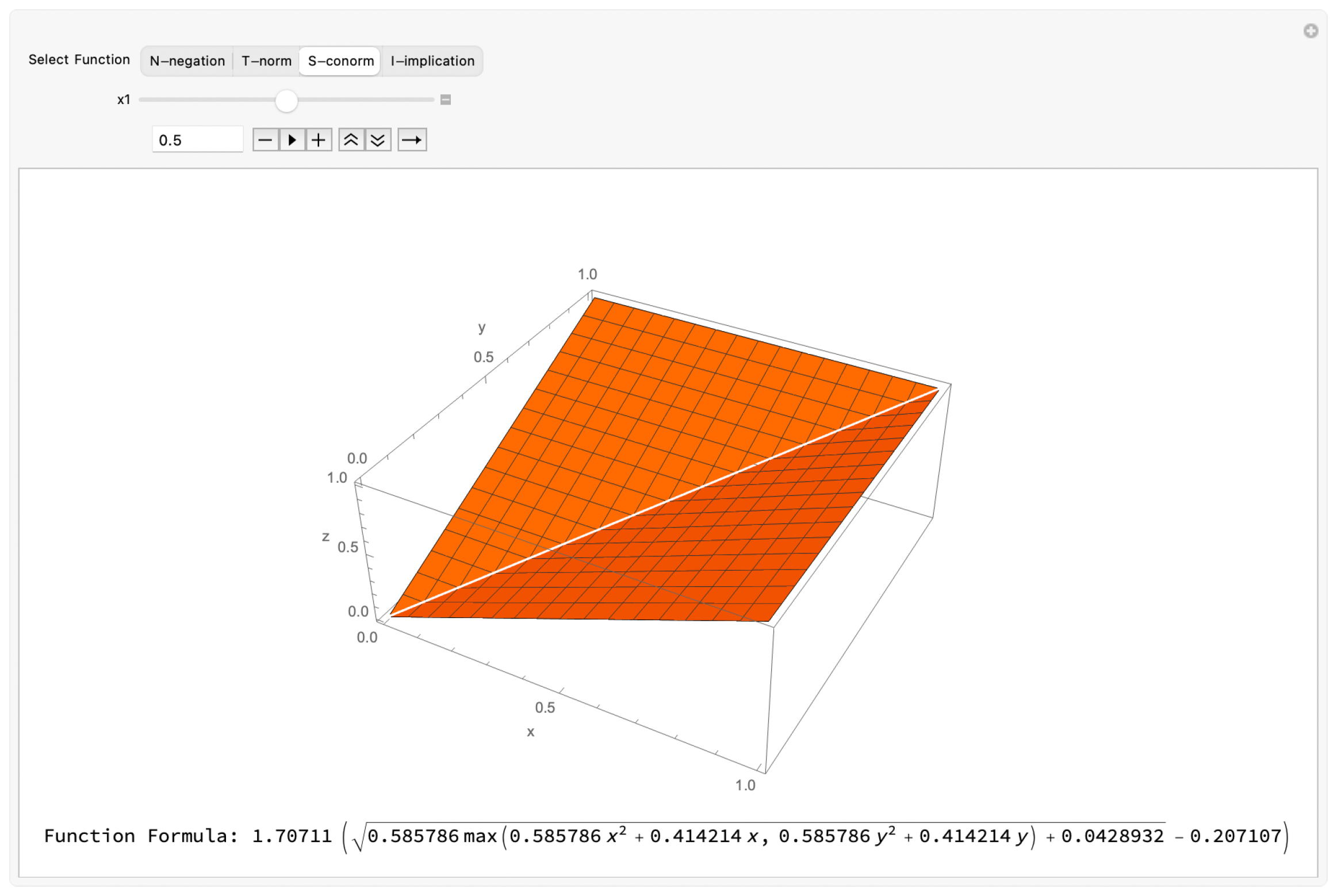
In Example 3, the maximum S-conorm is used as the input fuzzy connective. In this generator configuration, the maximum S-conorm can be replaced only by other S-conorms.

Example 3. 

Let $\phi :[0,1]\to [0,1]$ be a function with Formula (7).

Let ${\phi }^{-1}:[0,1]\to [0,1]$ be the inverse function of φ with Formula (8).

Let $S:{[0,1]}^2\to [0,1]$ be a S-conorm with the formula: $S(x,y)=max\{x,y\}$.

Then, there is a function $S\phi :{[0,1]}^2\to [0,1]$ with the formula:

$$S_{\phi }(x,y)=\frac{x_1-\sqrt{x_1}+\sqrt{{\left(x_1-\sqrt{x_1}\right)}^2+4·(max\{\frac{\sqrt{x_1}-1}{x_1-1}·x^2+\frac{x_1-\sqrt{x_1}}{x_1-1}·x,\frac{\sqrt{x_1}-1}{x_1-1}·y^2+\frac{x_1-\sqrt{x_1}}{x_1-1}·y\})·\left(1-x_1\right)·\left(1-\sqrt{x_1}\right)}}{2·\left(1-\sqrt{x_1}\right)}$$

(11)

where $x_1$ is a parameter with values ranging in the interval $(0,1)$.

Indeed,

utilizing Theorem 3 of [19], the formula $S_{\phi }(x,y)={\phi }^{-1}\left(S(\phi \left(x\right),\phi \left(y\right))\right)$ is applied.

Then, Equations (7) and (8)as well as the S-conorm are replaced in the formula:

$\begin{array}{c}{S}_{\phi }(x,y)={\phi }^{-1}\left(S(\phi \left(x\right),\phi \left(y\right))\right)\iff S_{\phi }(x,y)=\frac{x_1-\sqrt{x_1}+\sqrt{{\left(x_1-\sqrt{x_1}\right)}^2+4·\left(S(\phi \left(x\right),\phi \left(y\right))\right)·\left(1-x_1\right)·\left(1-\sqrt{x_1}\right)}}{2·\left(1-\sqrt{x_1}\right)}\iff \\ S_{\phi }(x,y)=\frac{x_1-\sqrt{x_1}+\sqrt{{\left(x_1-\sqrt{x_1}\right)}^2+4·(max\{\phi \left(x\right),\phi \left(y\right)\})·\left(1-x_1\right)·\left(1-\sqrt{x_1}\right)}}{2·\left(1-\sqrt{x_1}\right)}\iff \\ S_{\phi }(x,y)=\frac{x_1-\sqrt{x_1}+\sqrt{{\left(x_1-\sqrt{x_1}\right)}^2+4·(max\{\frac{\sqrt{x_1}-1}{x_1-1}·x^2+\frac{x_1-\sqrt{x_1}}{x_1-1}·x,\frac{\sqrt{x_1}-1}{x_1-1}·y^2+\frac{x_1-\sqrt{x_1}}{x_1-1}·y\})·\left(1-x_1\right)·\left(1-\sqrt{x_1}\right)}}{2·\left(1-\sqrt{x_1}\right)}\end{array}$ where $x_1$ is a parameter with values ranging in the interval $(0,1)$.

The graph of the generalized s-conorm $S_{\phi }$ when a parameter $x_1=0.5$ shown in the Figure 7.

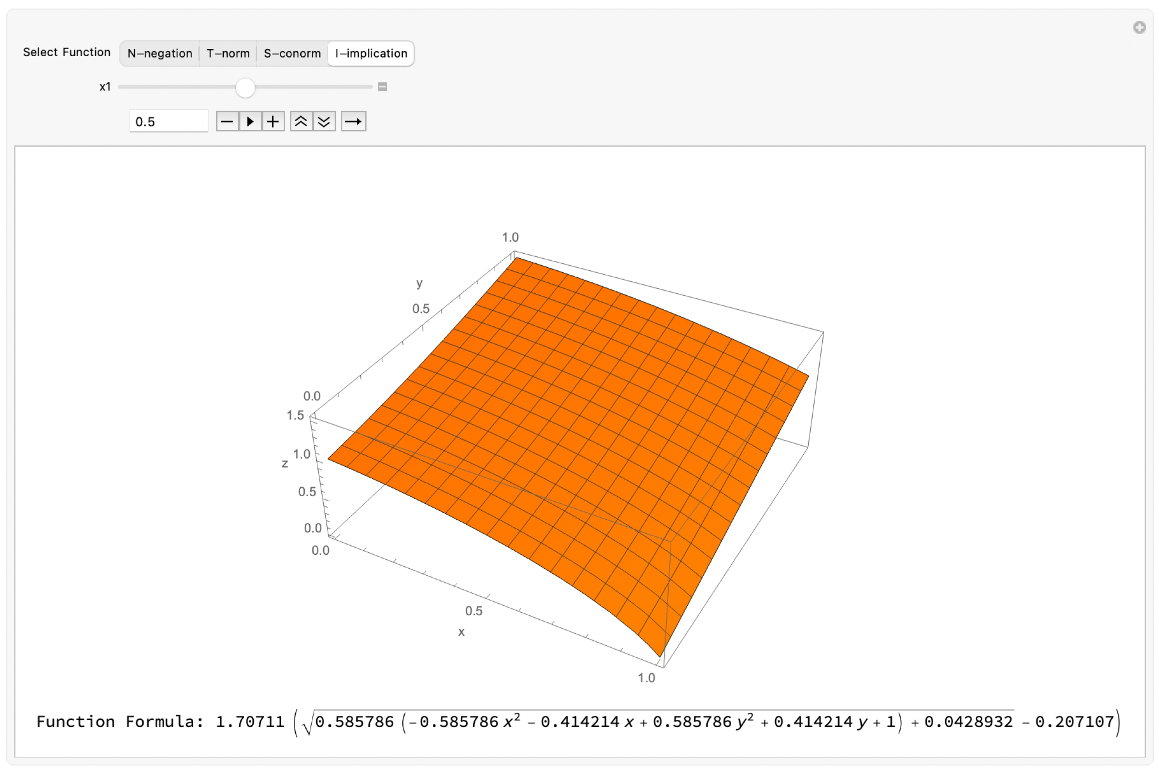
In Example 4, the Łukasiewicz I-implication is used as the input fuzzy connective. In this generator configuration, the Łukasiewicz I-implication can be replaced only by other I-implications.

Example 4. 

Let $\phi :[0,1]\to [0,1]$ be a function with Formula (7).

Let ${\phi }^{-1}:[0,1]\to [0,1]$ be the inverse function of φ with Formula (8).

Let $I:{[0,1]}^2\to [0,1]$ be a Łukasiewicz I-implication with formula: $I(x,y)=min\{1,1-x+y\}$.

Then, there is a function $I_{\phi }:{[0,1]}^2\to [0,1]$ with the formula:

$$I_{\phi }(x,y)=\frac{x_1-\sqrt{x_1}+\sqrt{{\left(x_1-\sqrt{x_1}\right)}^2+4·(min\{1,1-\frac{\sqrt{x_1}-1}{x_1-1}·x^2-\frac{x_1-\sqrt{x_1}}{x_1-1}·x+\frac{\sqrt{x_1}-1}{x_1-1}·y^2+\frac{x_1-\sqrt{x_1}}{x_1-1}·y\})·\left(1-x_1\right)·\left(1-\sqrt{x_1}\right)}}{2·\left(1-\sqrt{x_1}\right)}$$

(12)

where $x_1$ is a parameter with values ranging in the interval $(0,1)$.

Indeed,

utilizing [27], the formula $I_{\phi }(x,y)={\phi }^{-1}\left(I(\phi \left(x\right),\phi \left(y\right))\right)$ is applied.

Then, Equations (7) and (8), as well as the I-implication are replaced in the formula:

$\begin{array}{c}{I}_{\phi }(x,y)={\phi }^{-1}\left(I(\phi \left(x\right),\phi \left(y\right))\right)\iff I_{\phi }(x,y)=\frac{x_1-\sqrt{x_1}+\sqrt{{\left(x_1-\sqrt{x_1}\right)}^2+4·\left(I(\phi \left(x\right),\phi \left(y\right))\right)·\left(1-x_1\right)·\left(1-\sqrt{x_1}\right)}}{2·\left(1-\sqrt{x_1}\right)}\iff \\ I_{\phi }(x,y)=\frac{x_1-\sqrt{x_1}+\sqrt{{\left(x_1-\sqrt{x_1}\right)}^2+4·(min\{1,1-\phi \left(x\right)+\phi \left(y\right)\})·\left(1-x_1\right)·\left(1-\sqrt{x_1}\right)}}{2·\left(1-\sqrt{x_1}\right)}\iff \\ I_{\phi }(x,y)=\frac{x_1-\sqrt{x_1}+\sqrt{{\left(x_1-\sqrt{x_1}\right)}^2+4·(min\{1,1-\frac{\sqrt{x_1}-1}{x_1-1}·x^2-\frac{x_1-\sqrt{x_1}}{x_1-1}·x+\frac{\sqrt{x_1}-1}{x_1-1}·y^2+\frac{x_1-\sqrt{x_1}}{x_1-1}·y\})·\left(1-x_1\right)·\left(1-\sqrt{x_1}\right)}}{2·\left(1-\sqrt{x_1}\right)}\end{array}$where $x_1$ is a parameter with values ranging in the interval $(0,1)$.

The graph of the generalized I-implication $I_{\phi }$ when a parameter $x_1=0.5$ shown in the Figure 8.

As it is apparent from the above examples, the strategy of using polynomial automorphisms for the generalization of fuzzy connectives is a multistage and technical procedure. So, in this paper, mathematical modeling was employed for the purpose of automating the theorems as an efficient, reliable, and practical tool that streamlines the whole process from start to finish. In order to achieve this goal, two different paths during the development of the tool were taken. To be more specific: the tool was coded in two different programming languages and philosophies, which, even though they provide the same end results, prioritize different aspects.

The first version of the tool was coded in the programming language “MATLAB” using the version 2021b of the product “MATLAB”, which is distributed by the company MathWorks. Before explaining the mentioned code, it is important to state that it has been saved in a public repository and is accessible at Supplementary Materials.

The complexity and size of the code may be a problem for researchers that are not familiar with computer programming. As a result, it was deemed necessary to provide a simpler and more-accessible version of the project written in pseudo code.

The pseudo code version of the “MATLAB” script in steps is given as follows:

• Step 1: Create the points that will be used in the Lagrange interpolation as X and Y vectors;
• Step 2: Implement the Lagrange interpolation algorithm;
• Step 3: Display the messages to the user regarding the results of Step 2;
• Step 4: Create and display the Lagrange interpolating polynomial;
• Step 5: Display the automorphism properties to the user for the verification of its validity;
• Step 6: Create and display of the inverse Lagrange interpolating polynomial;
• Step 7: Plot the polynomial automorphism and its inverse;
• Step 8: Display the generalization menu to the user;
• Step 9: Generalize and plot the chosen fuzzy connective.

Since the basic structure of the script has been presented, in the following paragraphs, a more-detailed explanation of the procedures and user interface used is give. Moreover, the instructions for the proper use and modification of the code are given so other researchers can maximize the utility of the research presented in this paper.

The code has a very simple, yet practical user interface. Firstly, upon running the program, the user will be requested to input a float number between the numbers 0 and 1. If the input code is not valid, the program will not continue and the process will be repeated until the user provides the expected values. When this happens, the code automatically starts the implementation of Theorem 1 by creating the set of points that will be used in the Lagrange interpolation. Then, the Lagrange interpolation is executed. The code snippet responsible for the code implementation of the Lagrange interpolation was retrieved from [28]; however, it has been modified to fit the goals and practices of this study. The output of the interpolation is a vector, which includes the coefficients of the generated second-degree polynomial. This vector is displayed to the user among the abscissas and ordinates of the points used in the Lagrange interpolation. Then, using the tools of the MATLAB environment, the vector is converted into a symbolic function that houses the automorphism function. Afterwards, the automorphism properties of the polynomial are displayed, which include the calculation and plotting of the derivative of the polynomial. Furthermore, the inverse of the polynomial automorphism is calculated, and it is plotted with the polynomial.

At this point, the user is met with a menu of options regarding the generalization of fuzzy connectives. Specifically, the user has to choose between the generalization of one of the four categories of fuzzy connectives or the termination of the program. As before, any invalid input of the user will lead to a repeat of the process. If one of the four categories of fuzzy connectives is chosen, the program creates an indicative fuzzy connective as in Examples 1, 2, 3, and 4 and stores it in a symbolic function. It is important to highlight that the fuzzy connectives that are used can be replaced by any other compatible fuzzy connective, with the choice presented in this paper being made for illustration purposes. Any researcher that is interested in using the tool can easily change the input fuzzy connective from the source code (the lines that the user can modify are pointed out with comments inside the code, e.g., line 83). Then, the appropriate formula for the generalization of fuzzy connectives via automorphisms is used in combination with the generated polynomial automorphism, its inverse, and the fuzzy connective. The generated connective is displayed and plotted either as a regular plot or as a 3D plot depending the fuzzy connective category.

The main philosophy of this approach is the fact that the code simplifies the process of the generalization of fuzzy connectives and guides the user throughout it. To be more specific, the user will generate a specific automorphism and, gradually, without any effort, will be provided with all the necessary information regarding the specific generalization that he/she intends to realize.

The second version of the tool was coded in the programming language “Wolfram Language” using the version 12 of the product “WOLFRAM MATHEMATICA”, which is distributed by the company “WOLFRAM”. The code is also available at Supplementary Materials. The main philosophy of the approach taken in this code is the visualization of the research presented in this paper and not the creation of a streamlined process. The motivation behind the development of this project was the creation of a tool capable of providing a visual representation of the paper’s research that can be used and understood by any reader regardless of background. In order to achieve this, the program was divided into two independent sections, one focused on the presentation of the generated polynomial automorphisms and the other on the presentation of the generalized connectives.

In the first section, the code utilizes the general formulas (7 and 8, respectively) of the polynomial automorphism and its inverse as they were defined by Theorem 1 in order to create the respective plots. However, the program does not simply display the plots of these functions, as a more-elaborate user interface has been created. To be more specific, the plots have been labeled with the functions they represent and categorized into an easy-to-understand menu. Furthermore, each graph has its own unique color and a separate box that displays the specific function formula generated with every $x_1$ value. $x_1$ is defined by the user with the help of a slider, which simplifies the process even more. Moreover, a set of controls was implemented in the code that give the user the ability to influence the $x_1$ slider in multiple ways. For example, the user may choose to replace automatically different $x_1$ values in order to see the deviations between the unique generated polynomials. Finally, the menu presents the option of plotting the two functions on the same axis with all the above options being available.

In the second section, the code utilizes the generalized parametric Formulas ((9), (10), (11), and (12), respectively) as defined by Examples 1–4 in order to create the respective plots. The generalized parametric formulas used can be replaced by the generalized parametric formulas of any other compatible fuzzy connective, with the choice presented in this paper being made for illustration purposes. If a researcher wants to utilize the tool in order to visualize his/her own generalized fuzzy connective, he/she can follow the steps presented in the above-mentioned examples with the fuzzy connective of his/her choice in order to create the appropriate generalized fuzzy formula. The user interface and the various features of the program are the same as the above code, with the difference being that the majority of the plots are 3D and, as a result, were graphed in a different environment using the same color for visualization purposes.Finally, a third Mathematica script was created that was used to generate Figure 1, which displays the basic automorphism functions.

4. Results

The goal set at the start of the paper was the creation of a new method for generalizing fuzzy connectives using polynomial automorphisms. However, in order to achieve this target, it was necessary to generate the polynomial automorphisms, a task that was fulfilled with the composition of a strategy that involved numerical analysis. The results drawn from this research are represented in the following paragraphs.

4.1. Generation of Polynomial Automorphisms

The generation of polynomial automorphisms that satisfy the special criteria for use in fuzzy logic has proven to be a very demanding endeavor. However, the process displayed in this paper proved to be reliable and robust, as it is capable of generating an infinite number of unique polynomial automorphisms. Furthermore, two computer programs were constructed that automate the above-mentioned strategy into a procedure that can be operated by a researcher of any field. So, it is safe to say that the attempt to create a polynomial automorphism generator was successful.

4.2. Generalization of Fuzzy Connectives

Since the required automorphisms were successfully generated, the next step during the development process of this paper was the generalization of fuzzy connectives. In order to establish that the proposed method of generalization is valid, an indicative fuzzy connective was generalized from each fuzzy connective category. It is important to note at this point that the method can generalize any fuzzy connective; however, it is not possible to display the generalization of every fuzzy connective in a paper. The results of every generalization process were positive. As a result, the method presented in this paper was confirmed to work with any category of fuzzy connectives. Finally, the option of automating the generalization of the fuzzy connectives was added to the above-mentioned programs, leading to the creation of an efficient implementation of the introduced generalization method.

The main results of the paper can be briefly described as follows: a new powerful and robust polynomial automorphism generator was created; two programs were coded that automate both the generation of the polynomial automorphisms and the generalization of fuzzy connectives; a new, more-flexible method for generalizing fuzzy connectives was composed and proven.

5. Discussion

The results of the research presented in this paper provide a fresh view of the study of fuzzy connectives. One of the reasons that contributed to this is the fact that the generalization method proposed innovates in comparison with previous studies. To be more specific, every previous attempt at generalizing fuzzy connectives had turned to the use of alternative fuzzy connectives as a generalizing element. However, in this paper, the prospect of using a polynomial automorphism instead of a basic one was explored and validated, a choice that differentiated the method from any other that preceded it. Another reason is the fact that computer programming was employed to reinforce and automate the findings of the paper, a move that introduced new capabilities to the study of fuzzy connectives like the easy and accurate visualization of research. Furthermore, the discovery made in this paper opens the possibility of using numerical analysis as a potential tool in the study of fuzzy logic. Moreover, it is important to point out the fact that the generalized fuzzy connectives that were created by this paper are a very powerful and useful asset to the researchers that are active in fields like decision-making, artificial intelligence, and even environmental study like [29,30]. It is important also to mention that the use of second-degree polynomials in the process of generalization saved valuable processing resources and significantly reduced the complexity of the whole procedure, helping its widespread adoption. Finally, the utilization of degree polynomials highlights the future research direction of generating polynomial automorphisms of various powers.

6. Conclusions

This paper successfully tackled the problems and failings that led to its creation. Furthermore, it delivered useful and practical results that enable interesting future research directions. Furthermore, the presented research proved that computer programming can assist in the development of fuzzy connectives and fuzzy logic in general by automating tedious and repetitive tasks. In conclusion, taking everything this paper has researched into consideration, it is safe to assume that the study of fuzzy connectives not only is not near completion, but is at its infancy with exciting new opportunities becoming a reality.