Deep Learning-Based Cross-Layer Power Allocation for Downlink Cell-Free Massive Multiple-Input–Multiple-Output Video Communication Systems

Abstract

We propose a deep learning-based cross-layer power allocation method for asymmetric cell-free massive MIMO video communication systems. The proposed cross-layer approach considers physical layer channel state information (CSI) and the application layer rate distortion (RD) function, and it aims to enhance video quality in terms of peak signal-to-noise ratio (PSNR). Our study develops a decentralized deep neural network (DNN) model to capture intricate system patterns, enabling accurate and efficient power allocation decisions. The proposed cross-layer approach includes unsupervised and hybrid (supervised/unsupervised) learning models. The numerical results show that the hybrid method achieves convergence with just 50% of the iterations required by the unsupervised learning model and that it achieves a 1 dB gain in PSNR over the baseline physical layer scheme.

1. Introduction

Cell-free technology [1,2,3] enables the deployment of large-scale MIMO systems without cell boundaries, leading to enhanced network coverage, increased capacity, and reduced interference levels. This approach enables more flexible and efficient power allocation, leading to improved overall network performance.

The utilization of a cross-layer design [4,5,6,7] brings forth the benefits of effective collaboration between different layers of the wireless communication system. By integrating insights from the physical layer characteristics and user multimedia demands, we can optimize the power/resource allocation to reduce interference levels, resulting in improved user experience.

Deep learning [8,9,10,11] plays a crucial role in developing a learning-based power allocation model. By leveraging deep learning techniques, we can effectively capture complex patterns and correlations within the system, leading to more accurate and efficient power/resource allocation decisions [12,13,14,15].

By harnessing the advantages of cell-free technology, cross-layer design, and deep learning, this research aims to enhance the performance and applicability of cell-free massive MIMO (CFMM) systems. This should contribute to improved network coverage, increased capacity, and overall network performance in practical deployment scenarios.

The remaining part of this article is organized as follows. Section 2 presents previous related works. Section 3 outlines the contribution/novelty of this article. Section 4 introduces the system model. Section 5 presents the proposed solution. Section 6 discusses the proposed DNN model. Section 7 contains the simulation results. Section 8 presents our conclusions.

2. Related Works

In the field of CFMM systems, network coverage and feasibility have been challenging issues. The term “CFMM” was first introduced in [16]. Recent research, such as [2], has focused on the concept of a cell-free network and related technologies, providing essential information for designing and constructing next-generation mobile networks. Additionally, ref. [17] has proposed a scalable system framework to address these challenges.

Refs. [18,19] survey machine learning schemes for massive MIMO systems, including CFMM systems, in all practical implementations, such as precoding, power allocation, and channel estimation.

Building upon [20], another recent study, [21], introduced a fully distributed architecture that enhances the scalability and feasibility of cell-free networks. It also leverages deep neural networks (DNNs) to effectively reduce the overall system complexity. The experimental results demonstrated that its performance sacrifice is acceptable compared with those required for traditional optimal solutions.

Ref. [22] extends [21] and proposes a cooperative learning structure which is scalable to the number of APs in a CFMM network. Ref. [23] proposes a machine learning approach for power allocation in an underlay CFMM network.

However, these studies have focused on the physical layer only and have not considered both physical layer channel state information (CSI) and application layer rate distortion (RD) function. In this regard, the cross-layer solutions proposed in [4,5,24] have addressed this issue, providing better simulations of real-world usage scenarios.

3. Contributions

The contributions of this paper are outlined in this section. Ref. [21] developed a deep learning-based approach for computing downlink power allocation coefficients for a fully decentralized CFMM system using supervised learning. However, it considered the physical layer only. Unlike the physical layer baseline scheme presented in [21], we take a cross-layer approach and change the objective function to peak signal-to-noise ratio (PSNR), improving the video quality of CFMM video communication systems to improve user experience. We propose two schemes: unsupervised learning and hybrid (supervised/unsupervised) learning. For comparison, the baseline scheme of [21] applies supervised learning only and does not use hybrid (supervised/unsupervised) learning.

Both the proposed unsupervised learning method and the hybrid (supervised/unsupervised) learning method exhibit performance gains in cross-layer applications compared with the baseline scheme of [21]. The proposed hybrid learning method only needs 50% of the iterations required by the proposed unsupervised learning method to achieve convergence, and the resulting performance improvement is a 1 dB gain in video quality in terms of peak signal-to-noise ratio (PSNR) over the baseline physical layer scheme of [21].

4. System Model

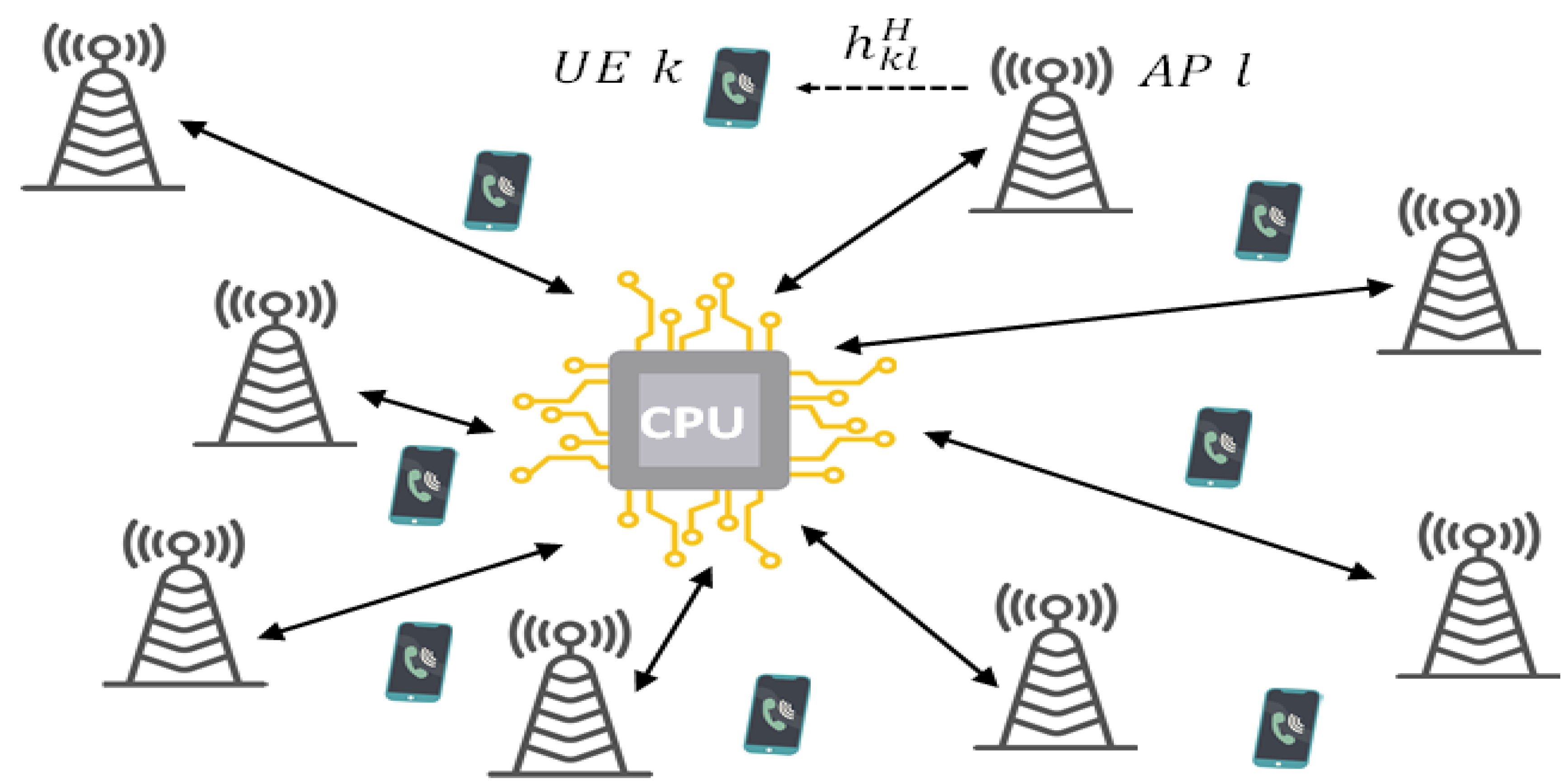
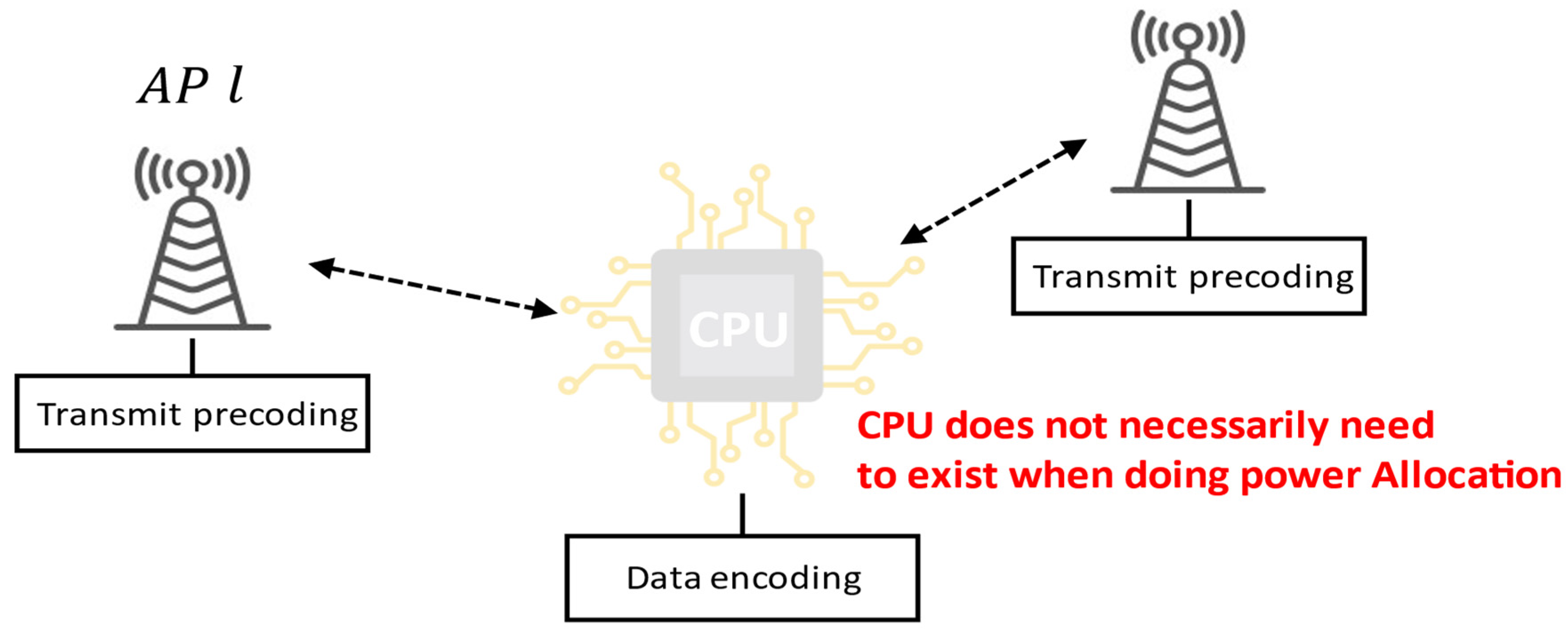
The cell-free network can be centralized, as in Figure 1, or distributed, as in Figure 2. Here, we consider a distributed cell-free network like the baseline scheme outlined in [21]. We consider a distributed cell-free network that has $K$ single-antenna user equipment (UE) distributed randomly over a wide service area. These UE devices are served simultaneously by $L$ access points (APs), each of which is equipped with N antennas. The channel model used assumes a standard block-fading approach, where the time-varying wideband channels are divided into coherence blocks to ensure that the channel time response remain stationary and the channel frequency response remains flat within each block [21]. Each coherence block comprises ${\tau }_c$ symbols, and within each block, the channels experience independent random variations. The communication channel connecting UE $k$ and AP $l$ is described as $h_{kl}$∈$C^{N\times 1}$ and adheres to a correlated Rayleigh fading model, where $h_{kl}$∼$N_c$(0, $R_{kl}$). In this context, $R_{kl}$∈$C^{N\times N}$ represents the spatial correlation matrix. The normalized trace ${\beta }_{kl}$ = $\frac{1}{N}$* tr($R_{kl}$) describes the average channel gain from a specific antenna at AP $l$ to UE $k$ [21].

Fronthaul links establish connections between APs and a central processing unit (CPU), facilitating the transmission of uplink (UL) and downlink (DL) data, along with other essential signals [19,25]. In the context of massive MIMO cell-free systems, precoding techniques are employed, involving the application of specific weightings to signals transmitted by different APs based on channel state information. This optimization reduces interference and enhances system performance [21]. This paper focuses on cross-layer power control in CFMM video transmission systems, ultimately boosting video quality performance [18,23].

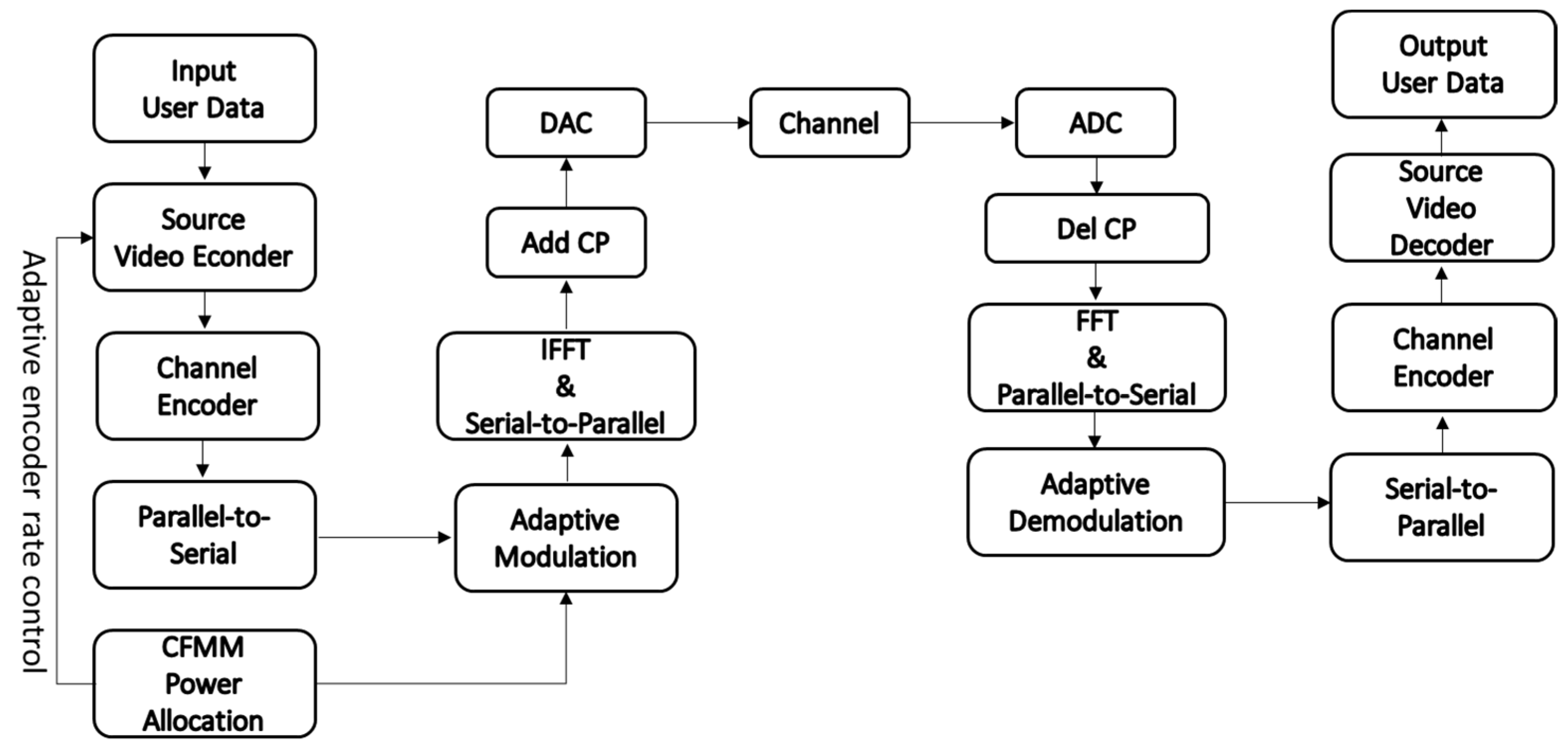
Figure 3 displays a block diagram depicting the CFMM video transmission system with cross-layer power allocation. It is similar to the cellular network video transmission system with cross-layer resource allocation described in [4,5,20], but it utilizes CFMM instead of cellular network communication and incorporates power allocation instead of resource allocation.

Cross-layer means a change of power allocation objective to PSNR. PSNR is a measure of video quality in the application layer. The proposed power allocation considers both PSNR (or the rate-distortion function) in the application layer and CSI in the physical layer and is thus a cross-layer approached as [4,5,6,20,24].

In addition, an adaptive source encoding rate (indicated by the arrow pointing to the video source encoder block in Figure 3) is employed to enhance video quality [4,5,20].

Downlink Data Transmission

In this scenario, we assume that all user equipment (UE) is served simultaneously by all access points (APs) using the same time–frequency resources. Consequently, the downlink (DL) signal received by UE k can be expressed as follows [21]:

$$y_k^{dl}=\sum _{l=1}^L{h}_{kl}^H\sum _{i=1}^K\sqrt{{\rho }_{il}}{w}_{il}{s}_i+n_k$$

(1)

Within the system framework, the channel between UE $k$ and AP $l$ is represented by $h_{kl}\in C^{N\times 1};{ \rho }_{il}$ ≥ 0 indicates the allocated downlink (DL) power from access point (AP) $l$ to user equipment (UE) $i$. The normalized precoding vector $w_{il}$∈$C^{N\times 1}$ is utilized to ensure its normalization, satisfying the condition ${‖w_{il}‖}^2=1$. Additionally, $s_i$ represents the zero-mean signal directed towards user equipment i, while $n_k$∼$N_c(0,{\sigma }^2)$ denotes complex Gaussian noise.

Based on the derivation presented in [25], the achievable spectral efficiency (SE) for user equipment (UE) k can be lower bounded by the following expression:

$${SE}_k=\frac{{\tau }_d}{{\tau }_c}(1+{SINR}_k)$$

(2)

where ${\tau }_d$ represents the duration of the downlink occupancy, while ${\tau }_c$ represents the duration of the entire coherence block. Since we are considering the downlink channel, we calculate the time ratio for the downlink portion.

5. Proposed Solution

In this section, our primary emphasis lies in the pursuit of maximizing the average peak signal-to-noise ratio (PSNR) by optimizing power allocation across the complete network. Our main goal is to identify the power allocation coefficients {${\mathsf{\rho }}_{kl}$:∀k,l} for the downlink links that lead to the highest average PSNR, a measure of video quality. For AP, the power constraint is formulated:

$$\sum _{k=1}^K{\mathsf{\rho }}_{kl}\le P_{max}^{dl}$$

(3)

The power limitation for each AP is specified by the maximum permissible transmit power, denoted as $P_{max}^{dl}$.

5.1. Video Distortion MSE Model (RD Function) and PSNR

To simulate realistic usage scenarios, we adopted the video distortion MSE model in [4,5,20,24,26]. For each group of pictures (GOPs), representing a sequence of video frames, the video distortion MSE (or rate-distortion function, RD function) for the user $k$ is approximated as:

$${video distortion MSE}_k=a_k+\frac{b_k}{{\sum }_{l=1}^L{R}_{l,k}+c_k}$$

(4)

where the constants $a_l$, $b_l$ and $c_l$ are specific to the content of the video and will vary accordingly. Among them, $a_l$ represents the distortion introduced by video data compression. The term $\frac{b_k}{{\sum }_{l=1}^L{R}_{l,k}+c_k}$ represents the residual error and the error between video frames, where $R_{l,k}$ is the information rate (in bits/s) between the AP $l$ and the user $k$. For higher video complexity such as fast motion, $b_k$ is larger. The video source encoder (H.264 baseline profile) has seventeen discrete rates. These operation points corresponding to specific video encoding rates, were used to nonlinearly fit the video distortion MSE model/RD function in (4) [4,20,24,26].

The common user video quality peak signal-to-noise ratio (PSNR) is the reciprocal of the video distortion MSE [4,5,20,24,26]. The PSNR for user k is:

$$\mathrm{P}\mathrm{S}\mathrm{N}{R}_k=10{\mathit{log}}_{10}\left(\frac{{255}^2}{video distortion MS{E}_k}\right)$$

(5)

where 255 is the peak signal because one pixel is of 8 bits (0–255) in H.264 source encoding.

The average PSNR (averaging over the users’ PSNR/video quality), which will be used in the loss function in the unsupervised learning in (15), is:

$$\mathit{\text{avg\_PSNR}}=\frac{1}{K}\sum _{k=1}^K{PSNR}_k$$

(6)

5.2. Baseline Scheme: Physical Layer

Ref. [21] proposes a fully distributed DNN learning framework in a massive MIMO cell-free system. The model is trained to maximize the system’s total spectral efficiency, the objective function, using SINR. This model incorporates a supervised learning approach by generating labels through WMMSE. The labels are then utilized in the training process to optimize the performance of the deep neural network. The spectral efficiency is computed using (2) to determine the achievable rate in the system.

$$\underset{\{{\mu }_{\mathit{kl}} : \forall k,l\}}{\mathrm{maximize}}{\log }_2(1+{SINR}_k)$$

(7)

$${\mathit{SINR}}_k=\frac{(a_k^T{\mu }_k{)}^2}{\sum _{i=1}^K{\mu }_i^T{B}_{ki}{\mu }_{i }-(a_k^T{\mu }_k{)}^2+{\mathsf{\sigma }}^2}$$

(8)

where

$${\mu }_k=[{\mu }_{k1}\dots { \mu }_{kL}{]}^T\in {\mathbb{R}}^{L\times 1},{ \mu }_{kl}=\sqrt{{\rho }_{il}}$$

(9)

$$a_k=[a_{k1}\dots { a}_{kL}{]}^T\in {\mathbb{R}}^{L\times 1},{ a}_{kl}=\mathbb{E}\{h_{kl}^H{w}_{kl}\}$$

(10)

$$B_{ki}\in {\mathbb{R}}^{L\times L},b_{ki}^{lm}=\mathfrak{R}\left(\mathbb{E}\right\{h_{kl}^H{w}_{il}{w}_{im}^H{h}_{km}\left\}\right)$$

(11)

Equation (7) represents the objective function, which is maximized to enhance the system’s total spectral efficiency using the signal-to-interference-plus-noise ratio (SINR).

Transmit power limit per AP:

$$Subjet to\sum _{k=1}^K{{\mu }^2}_{kl}\le P_{max}^{dl},l=1,\dots ,L$$

(12)

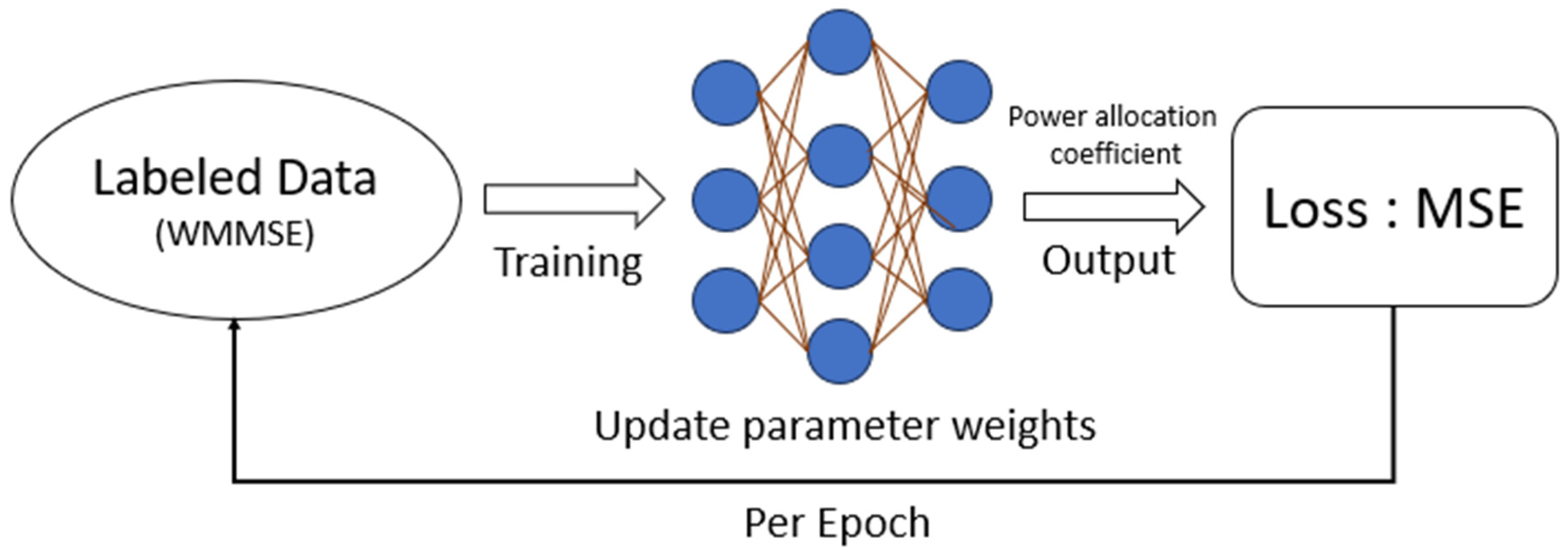
Figure 4 illustrates the training process of the baseline physical layer scheme [21] for supervised learning. Initially, labels for the power allocation coefficients are generated through WMMSE, and the weights are updated at each iteration.

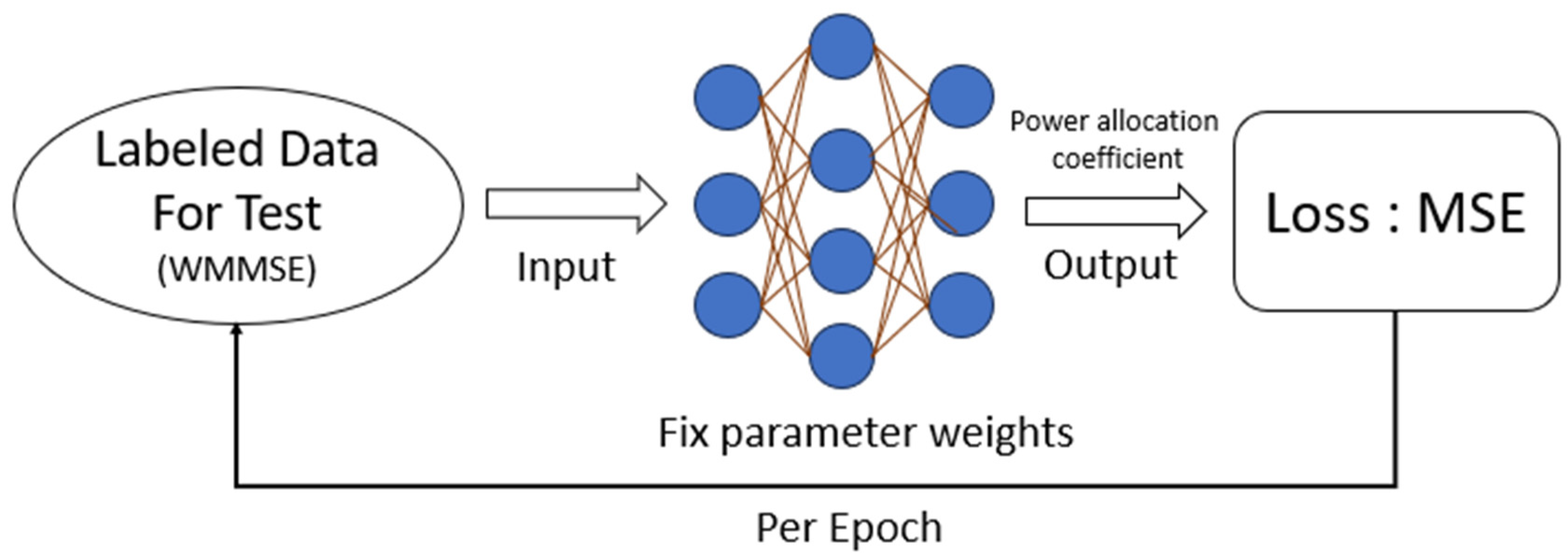
Figure 5 depicts the testing process of the baseline physical layer scheme [21] for supervised learning. The most significant difference between testing and training is that the weights are not updated; instead, they are used to directly produce corresponding outputs based on the respective inputs.

In order to gain a deeper understanding of the fundamental problem structure, ref. [21] introduces variables {${\mu }_{kl}$} in (12), which are related to the square roots of the power allocation coefficients {${\rho }_{il}$}. In this research, the optimization problems under consideration do not enforce constraints on ${\mu }_{kl}$ ≥ 0, following a similar approach as discussed in [25]. This relaxed formulation facilitates the derivation of analytical update formulas in the ensuing algorithms. Importantly, this relaxation does not lead to any complications since, upon completion of the optimization algorithms, any negative values of ${\mu }_{kl}$ can be seamlessly substituted with their positive counterparts without violating any other constraints.

5.3. Problem Formulation: Average-PSNR Maximization

When transmitting videos in a cell-free system, it becomes crucial to consider not only the theoretical communication capacity but also factors like video content and channel conditions for propagation. This comprehensive approach goes beyond considering only the data and channel statistics at the physical layer, as it also incorporates considerations of RD function/video distortion MSE in (4) at the application layer.

The problem is formulated as to maximized the average video quality, PSNR, as follows:

$$\underset{\{{\mu }_{\mathit{kl}} : \forall k,l\}}{\mathrm{maximize}} \mathit{\text{avg\_PSNR}}=\frac{{\sum }_{k=1}^K{PSNR}_k}{K}$$

(13)

$$Subjet to \sum _{k=1}^K{{\mu }^2}_{kl}\le P_{max}^{dl}, l=1,\dots ,L$$

(14)

6. Proposed DNN Model

Building upon the concept presented in [21], we have developed a fully distributed power allocation model for each access point (AP) using a deep neural network (DNN). This model relies solely on statistical information obtained from the local channels between the AP and various user equipment (UE), making it easily accessible at the AP. To enhance the system’s performance for users consuming diverse video and audio content, we have modified the loss function of this model to maximize the overall system’s average peak signal-to-noise ratio (PSNR). In response to this requirement, we have introduced both unsupervised and hybrid (supervised/unsupervised) learning approaches.

6.1. Proposed Scheme: Cross-Layer UL

For the unsupervised learning approach, we developed a model that does not rely on labeled data and instead utilizes the available statistical information from the local channels. This approach allows for autonomous learning and adaptation based on the observed patterns and characteristics of the system. The model was designed to address the objective of maximizing the overall system’s average PSNR, thereby enhancing the system’s performance for various video and audio content.

Similar to common approaches in maximizing problems, we can handle our objective function, defined as (13) and (14), by introducing a negative sign to it:

$$\mathit{Loss}=-\mathit{\text{avg\_PSNR}}=-\frac{{\sum }_{k=1}^K{PSNR}_k}{K}$$

(15)

To optimize the training process and focus on learning unknown variables, preprocessing the input data using domain knowledge is crucial. Instead of directly using the raw large-scale fading (LSF) coefficients as DNN inputs, to generate inputs, a heuristic approach is employed, utilizing the LSF coefficients to devise a power allocation scheme. This heuristic power allocation scheme is designed to optimize the distribution of inputs for the system. Our numerical experiments demonstrate that this heuristic method yields inputs with improved dynamic range and distribution, ultimately leading to the enhanced performance of the distributed DNN. The coefficients obtained through this heuristic approach are computed in a similar manner to the methodology outlined in [19].

$${{\rho }^{\prime }}_{il}=\sqrt{P_{max}^{dl}}\frac{{{(\beta }_{kl})}^v}{{\sum }_{i=1}^K{{(\beta }_{il})}^v }, k=1,\dots ,K$$

(16)

In the heuristic approach described in (16), we introduce the constant exponent $v$ to transform the large-scale fading (LSF) coefficients. An interesting aspect of this heuristic is its direct provision of the ratio between the LSF coefficients, which significantly influences power allocation decisions. By incorporating this heuristic input, we enhance the dynamic range and distribution of the dataset while retaining all pertinent information. In order to standardize the dataset, we use a robust scaler to normalize the logarithm (in dB scale) of the heuristic coefficients {${{\rho }^{\prime }}_{kl}$: ∀k}. This scaler employs the interquartile range, which measures the range between the first and third quartiles, to rescale the data. This method efficiently reduces the influence of outliers present in the dataset, caused by substantial variations in LSF coefficients among different user equipment (UE) for a given access point (AP), especially in larger coverage areas.

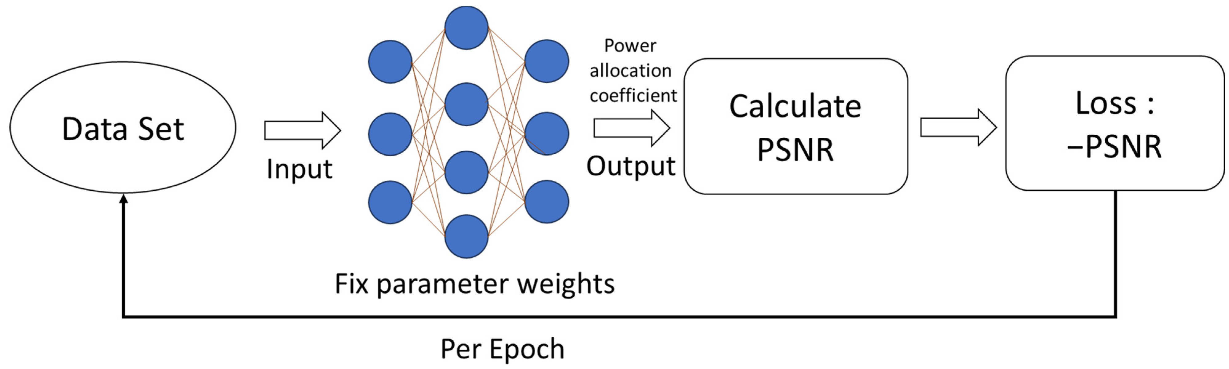
Figure 6 illustrates the training process of our proposed UL (unsupervised learning) approach. The dataset is fed into the DNN, and after each output, the result is transformed into the PSNR. This PSNR value is then negated and used as the loss function to update the model’s parameter weights due to the necessity of the PSNR transformation involving calculations from (4) to (6).

Figure 7 depicts the testing process of our proposed UL approach. The primary distinction between testing and training lies in the fact that the weights are not updated in reverse. Instead, they are utilized to transform the corresponding input into the PSNR, which serves as the corresponding output for evaluating the model’s performance.

Table 1. Fully distributed DNN architecture: 5524 trainable parameters.

	Dimension	Parameters	Activation Method
Input	K	-	-
Layer1	32	672	Linear
Layer2	64	2112	Tanh
Layer3	32	2080	Tanh
Layer4	K	660	Relu

illustrates the configuration of a fully distributed DNN. For an AP involves a set of parameters that need to undergo training. Specifically, there are 5524 parameters that will be fine-tuned during the training process. These parameters play a crucial role in the DNN’s ability to adapt and optimize power allocation based on the local channel characteristics. Through iterative updates and optimization, the DNN learns to make informed decisions about power allocation, aiming to maximize the system’s overall average PSNR. The training procedure enables the DNN to effectively leverage the available data and optimize its parameter values for improved performance.

6.2. Proposed Scheme: Cross-Layer Hybrid (SL/UL)

In our hybrid (supervised/unsupervised) learning approach, we have adopted a methodology similar to the one used in [20], with supervised learning in the first stage and unsupervised learning in the second stage for fine-tuning. This hybrid method combines labeled and unlabeled data to harness the strengths of both approaches. By leveraging the labeled information and incorporating a larger pool of training data, our goal is to enhance the model’s performance and generalization ability. The model’s architecture adheres to the approach outlined in UL, with the layout designed as per Table 1.

The model is divided into two stages. In the initial stage, we persist with the methodology proposed in [21], where the objective function aims to maximize the supervised deep neural network (DNN) learning of sum-SE. Convergence is typically attained within around 50 epochs. In this stage, our loss function is designed using mean squared error (MSE); during the training process, the DNN for access point (AP) $l$ is optimized to minimize the following loss function:

$$\mathit{Loss}=‖{\overline{\mathsf{\mu }}}_l^{\ast }-{\overline{\mathsf{\mu }}}_l^{DNN}‖$$

(17)

The vector ${\overline{\mathsf{\mu }}}_l^{\ast }$ = ${\left[{\overline{\mathsf{\mu }}}_{1l}^{\ast },\dots {\overline{\mathsf{\mu }}}_{Kl}^{\ast }\right]}^T$ represents the concatenation of the optimal normalized powers (obtained using the WMMSE approach) to disseminate the total power allocated by the access point (AP) to all user equipment (UE) across the network.

Following the initial 50 epochs, where the model was updated based on supervised learning (SL), despite the objective not directly focusing on the PSNR, the model’s parameters can still benefit from the labels generated through the weighted minimum mean squared error (WMMSE) approach. In the subsequent second stage of training, we will continue updating the model’s parameters using unsupervised learning. The loss function used will remain the same as (15).

7. Simulation Result

The simulation parameters, extracted from [21], are succinctly presented in

Table 2. Parameters for the simulation CFMM networks, similar to those in [21].

Coverage Area	1000 m × 1000 m
Bandwidth	20 MHz
AP Count	L = 16
UE Count	K = 20
Antenna Count per AP	N = 4
Pathloss Factor	α = 3.76
DL Transmit Power Limit per AP	$P_{max}^{dl}$ = 1 W
Uplink Transmit Power	$p_i$ = 100 mW
Noise Power (UL/DL)	−94 dBm

. We investigated a cell-free network encompassing 16 access points (APs) denoted by L, strategically deployed in an expansive area measuring 1000 m × 1000 m. Each AP is equipped with four antennas (N = 4). To create a realistic simulation, we employed a wrap-around topology to eliminate artificial boundaries. Moreover, we randomly and uniformly distributed 20 user equipment (UE) devices (K = 20) within the coverage area. To ensure the reliability and consistency of the findings, the performance outcomes were averaged over an extensive and diverse test dataset that consists of 6000 different user equipment (UE) distributions. It is essential to note that this test dataset is entirely distinct and separate from the training dataset, which greatly contributes to the model’s ability to generalize effectively to unseen scenarios.

Communication is conducted over a 20 MHz channel, and the total power of the receiver noise is −94 dBm. Each access point (AP) is capable of transmitting a maximum downlink power of $P_{max}^{dl}$ = 1 W, while each user equipment (UE) device employs an uplink power of $p_i$ = 100 mW during the pilot transmission phase. The system follows the approach presented in [25], wherein the entire bandwidth is shared among all APs, resulting in an average bandwidth of 1.25 MHz per AP under normal conditions. The LSF coefficients are generated using the pathloss model based on the methodology described in [27,28].

The parameters of the dataset are provided in

Table 3. Parameters of the datasets.

Algorithm	Dataset Size (Samples)	Features	Training	Testing
Baseline 1 [21]	200,000	CSI	190,000	10,000
Baseline 2 [22]	200,000
Proposed UL	400,000		390,000	10,000
Proposed Hybrid	400,000

. For the baseline methods [21,22], the dataset of 200,000 samples is divided into training and testing sets, with the training set containing 190,000 samples and the testing set including 10,000 samples. For our proposed UL method and hybrid method, we employed a larger dataset, each containing 400,000 samples. The testing dataset has the same 10,000 samples.

The simulation platforms/tools we used are a desktop PC with Intel Core i7-10700 K CPU and 24 GB of RAM and Zotac (China) RTX 3060 GPU, and Pytorch version 1.9.0.

In Section 7.1, we compare the results of different models in terms of their performance on the test data. In Section 7.2, we extensively compare unsupervised and hybrid (supervised/unsupervised) learning models, focusing on the peak signal-to-noise ratio (PSNR) during training and testing. In Section 7.3, we compare the complexity. In Section 7.4, we compare the performance in massive MIMO cases.

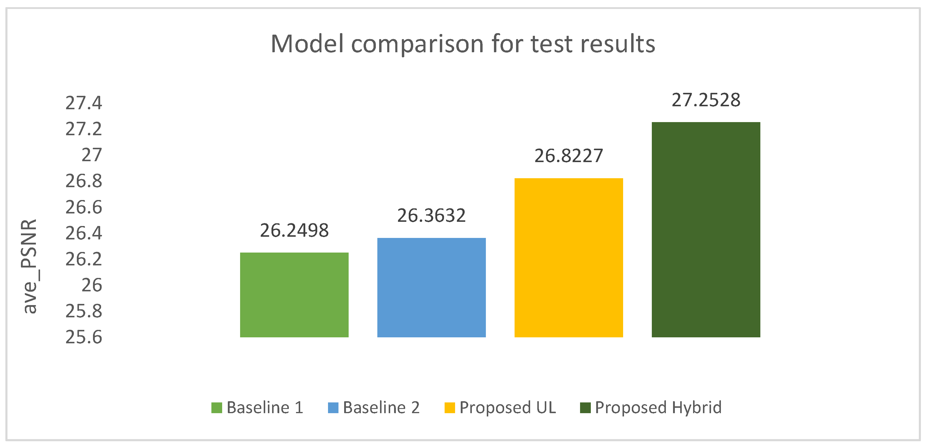
7.1. Model Comparison for the Test Results

In this section, we compare the results of different models in terms of their performance on the test data. We evaluate the models based on various metrics and analyze their effectiveness in solving the given problem. The models under consideration include:

• Baseline 1 [21]: This model serves as the reference or baseline model. It represents a supervised learning approach with the objective function of minimizing the sum of squared errors (sum-SE).
• Baseline 2 [22]: Another physical layer scheme has improved spectrum efficiency over physical layer scheme Baseline 1 [21]
• Proposed UL-cross: This model utilizes an unsupervised learning approach and aims to maximize the average PSNR (peak signal-to-noise ratio) of the entire network.
• Proposed Hybrid (SL/UL)-cross: This model adopts a hybrid approach combining both supervised and unsupervised learning methods. It integrates elements of both supervised and unsupervised learning, utilizing labeled data borrowed from Model SL-phy to update the model parameters, and further incorporating unsupervised learning similar to Model UL-cross. The objective function of the model is to maximize the average PSNR of the network. It follows a two-stage training approach.

We evaluated and compared these models based on their respective objective functions and their performance in terms of average PSNR. The results, as shown in Figure 8, indicate that both Model UL-cross and Model Hybrid (SL/UL)-cross outperform Model SL-phy in maximizing the average PSNR of the network.

Therefore, Model UL-cross and Model Hybrid (SL/UL)-cross demonstrate better effectiveness in addressing the objective of maximizing the average PSNR compared to the reference Model SL-phy.

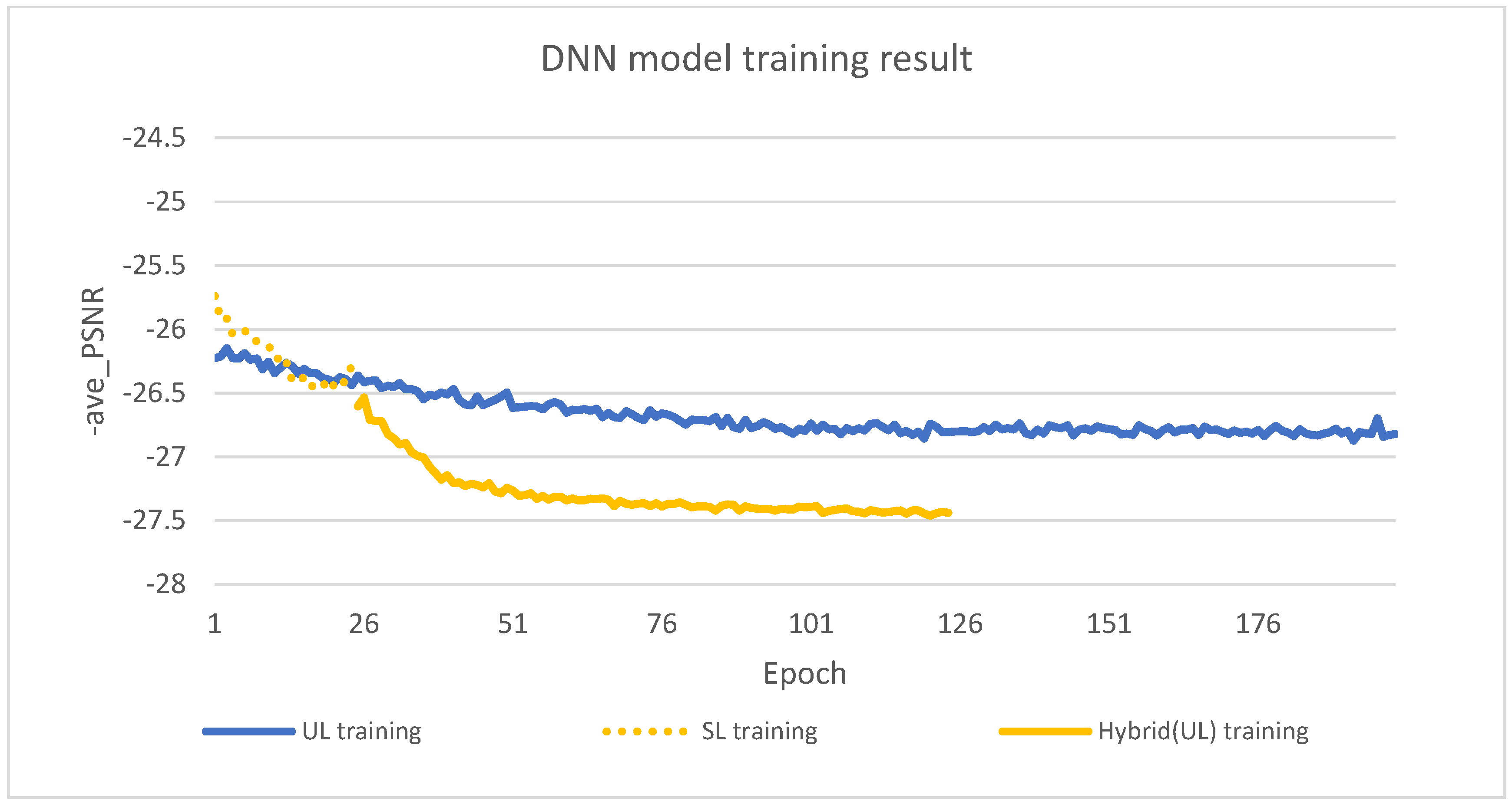
7.2. Model UL vs. Model Hybrid (SL/UL)

In this section, we extensively compared unsupervised and hybrid (supervised/unsupervised) learning models, focusing on the peak signal-to-noise ratio (PSNR) during training and testing. The hybrid model consistently outperformed the unsupervised model, showing higher PSNR values throughout. This showcases the effectiveness of combining supervised and unsupervised learning.

During testing, both models experienced a slight performance decrease, which is common in deep learning. The hybrid model stood out with impressive generalization, maintaining results close to its training performance. This indicates its robustness and reliability in real-world scenarios.

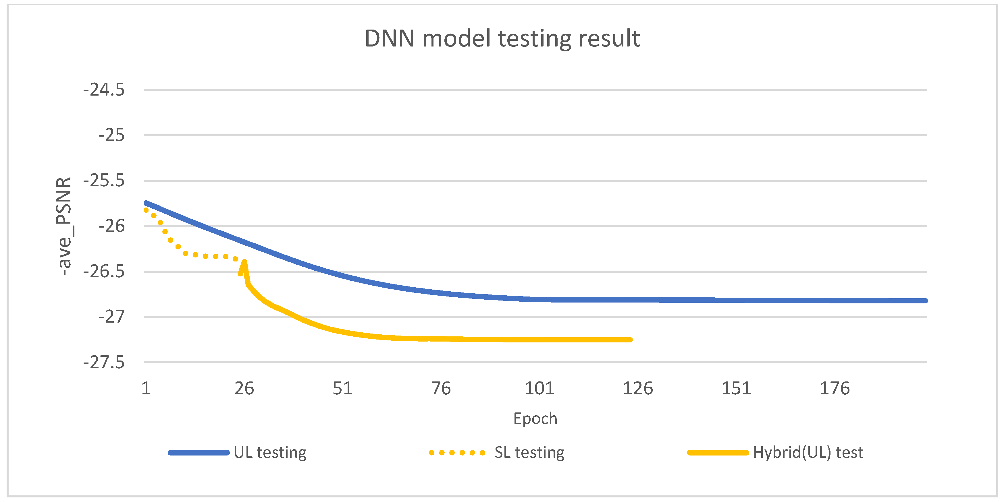
Figure 9 shows the loss function evolution during training, while Figure 10 displays changes in the loss function during testing. Our analysis focuses on evaluating the model’s performance based on the testing results.

According to the observations from Figure 10, the hybrid learning (supervised+ unsupervised two stage) method shows a significant improvement in PSNR compared to pure unsupervised learning. This finding is further supported by the fact that during the initial training phase of hybrid methods, the goal is to maximize the sum SE of the system. Surprisingly, this goal also gradually improves the overall PSNR of the system. Hence, hybrid learning methods are proven to be very effective in achieving better performance.

Pure unsupervised learning usually takes about 150 iterations to converge, and the hybrid method has a clear advantage in training time. It only requires about 25 iterations of supervised learning, followed by 50 iterations of unsupervised learning. The hybrid learning method saves about 75 iterations compared to the unsupervised learning method, thus greatly reducing the training time. Remarkably, this hybrid approach requires only 50% of the iterations of unsupervised learning, while still achieving superior performance.

7.3. Complexity and Performance Comparison

In

Table 4. Comparison of complexity and PSNR values.

Schemes	Average Computational Time (ms) at Testing Stage	PSNR (dB)
Baseline physical layer [21]	9.134	26.2498
Baseline physical layer [22]	9.173	26.3632
Proposed cross-layer UL	9.168	26.8227
Proposed cross-layer hybrid	10.189	27.2528

, we present performance and execution time comparisons between our proposed cross-layer UL and hybrid methods against the baseline physical layer schemes [21,22]. It can be observed that after model training is completed, there is actually little difference in execution time among the various models at the testing stage. This is because the sizes of the DNNs of the proposed schemes and baseline schemes are similar, falling within the range of approximately 9 to 10 ms. Therefore, in terms of complexity, our two proposed methods do not exhibit significantly higher complexity compared to [21,22].

Comparing Figure 4 and Figure 5 and Figure 6 and Figure 7, respectively, the cross-layer approach has additional PSNR calculation, so the computational burden is slightly higher, as also verified in the execution time in Table 3.

Furthermore, in terms of video quality, PSNR values, it can also be observed that both of our proposed methods outperform other methods [21,22]. This improvement is attributed to the fact that our models are optimized specifically with the PSNR as the objective function.

7.4. Performance Comparison in Massive MIMO Cases

In this subsection, we compare the baseline scheme [21] and the proposed cross-layer hybrid in massive MIMO cases, where the number of antennas is 64 or higher. As shown in

Table 5. PSNR performance comparison with larger number of antennas, N = 4,32,256. Baseline 1 is [21], a physical layer scheme.

Schemes	Number of AP Antennas	PSNR (dB)
Baseline 1	4	26.2498
Baseline 1	32	26.2589
Baseline 1	256	26.2723
Proposed cross-layer hybrid	4	27.2528
Proposed cross-layer hybrid	32	27.3373
Proposed cross-layer hybrid	256	27.5238

, the proposed cross-layer hybrid outperforms the baseline scheme [21] by 1.2515 dB when the number of antennas N = 256. The performance gain is larger than 1.0030 dB when the number of antennas N = 4

8. Conclusions

This study focused on addressing the power allocation problem in the downlink (DL) for CFMM systems. We adopted MR (maximum ratio) precoding for the task. Initially, we formulated the objective of maximizing the average PSNR (peak signal-to-noise ratio) across the network, as it provided the most suitable means to generate labels for learning. Consequently, we developed a DNN (deep neural network) architecture that combines unsupervised and hybrid (supervised/unsupervised) learning. This DNN architecture allowed us to approximate the power coefficients by solely utilizing locally available LSF (line spectral frequency) coefficients at the AP/EP (access point/edge point), effectively reducing the need for forward/backward transmissions.

Our proposed architecture outperforms the control group in maximizing the average PSNR across the network. Hybrid learning combines labeled and unlabeled data to improve model performance and generalization. The final experimental results indicate that the proposed approach also outperforms unsupervised learning.