Riemann–Hilbert Problems, Polynomial Lax Pairs, Integrable Equations and Their Soliton Solutions ^†

Abstract

The standard approach to integrable nonlinear evolution equations (NLEE) usually uses the following steps: (1) Lax representation $[L,M]=0$; (2) construction of fundamental analytic solutions (FAS); (3) reducing the inverse scattering problem (ISP) to a Riemann-Hilbert problem (RHP) ${\xi }^{+}(x,t,\lambda )={\xi }^{-}(x,t,\lambda )G(x,t\lambda )$ on a contour $\Gamma$ with sewing function $G(x,t,\lambda )$; (4) soliton solutions and possible applications. Step 1 involves several assumptions: the choice of the Lie algebra g underlying L, as well as its dependence on the spectral parameter, typically linear or quadratic in $\lambda$. In the present paper, we propose another approach that substantially extends the classes of integrable NLEE. Its first advantage is that one can effectively use any polynomial dependence in both L and M. We use the following steps: (A) Start with canonically normalized RHP with predefined contour $\Gamma$; (B) Specify the x and t dependence of the sewing function defined on $\Gamma$; (C) Introduce convenient parametrization for the solutions ${\xi }^{\pm }(x,t,\lambda )$ of the RHP and formulate the Lax pair and the nonlinear evolution equations (NLEE); (D) use Zakharov–Shabat dressing method to derive their soliton solutions. This requires correctly taking into account the symmetries of the RHP. (E) Define the resolvent of the Lax operator and use it to analyze its spectral properties.

1. Introduction

In 1968 one of the great discoveries in mathematical physics took place. Its authors: P. Lax, C. S. Gardner, J. M. Greene, M. D. Kruskal, R. M. Miura and N. J. Zabusky after several years of analysis proved that the KdV equation can be exactly solved by the inverse scattering method (ISM). This was the first and for some time, the only NLEE that could be solved exactly. Soon after, it was demonstrated that the KdV is a completely integrable infinite-dimensional Hamiltonian system; its action-angle variables were found by Zakharov and Faddeev [1]. The whole story is well described by N. J. Zabusky in his review paper [2].

The second big step in this direction followed in 1971 by the seminal paper of Zakharov and Shabat who discovered the second equation integrable by the ISM: the nonlinear Schrödinger (NLS) equation [3]; in 1973 the same authors demonstrated that the NLS equation is integrable also under non-vanishing boundary conditions [4]. Both versions of NLS equations described interesting and important physical applications in nonlinear optics, plasma physics, hydrodynamics and others. This inspired many scientists, mathematicians and physicists alike, to join the scientific community interested in the study of soliton equations. As a result, new soliton equations started to appear one after another. Notable mentions being the modified KdV (mKdV) equation [5], the N-wave equations [6], the Manakov system known also as the vector NLS equation [7] and many others. Many of them have already been included in monographs: see, e.g., [8,9,10,11,12] and the numerous references therein.

The first few NLEE were related to the algebra $sl\left(2\right)$, so the corresponding inverse scattering problem could be solved using the famous Gelfand-Levitan-Marchenko (GLM) equation. For the Manakov system, it was necessary to use the $2\times 2$ block matrix Lax operator, so the GLM equation was naturally generalized also for that case. However, the ISM for the N-wave system came up to be substantially more difficult. Indeed, for the $2\times 2$ (block) matrix Lax operator the Jost solutions possess analyticity properties, which are basic for the GLM equation. However, the Lax pair for the N-wave system is the generalized $sl\left(n\right)$ Zakharov–Shabat system (GZS):

$$\begin{array}{cc}\hfill L\psi & \equiv i\frac{\partial \psi }{\partial x}+([J,Q(x,t)]-\lambda J)\psi (x,t,\lambda )=0,M\psi \equiv i\frac{\partial \psi }{\partial t}+([K,Q(x,t)]-\lambda K)\psi (x,t,\lambda )=0,\hfill \\ \hfill J& =\mathrm{diag}(a_1,a_2,\dots ,a_n),K=\mathrm{diag}(b_1,b_2,\dots ,b_n),\hfill \end{array}$$

(1)

where $[X,Y]=XY-YX$ is the commutator of X and Y, $a_k$ and $b_k$ are real constants such that $trJ=0$, $trK=0$. Without restrictions, we can assume that $a_1>a_2>\dots >a_n$. In this case, only the first and the last columns of the corresponding Jost solutions allow analytic extension in the spectral parameter $\lambda$. This, however, was not enough to derive the GLM equation. It was Shabat who discovered the way out of this difficulty [13,14]. He was able to modify the integral equations for the Jost solutions into integral equations that provide the fundamental analytic solutions (FAS) ${\chi }^{+}(x,t,\lambda )$ and ${\chi }^{+}(x,t,\lambda )$ of L which allowed analytic extensions for $Im\lambda >0$ and $\mathrm{Im}\lambda <0$, respectively. As a result, the interrelation between the FAS and the sewing function $G_0(x,t,\lambda )$:

$$\begin{array}{cc}\hfill {\chi }^{+}(x,t,\lambda )& ={\chi }^{-}(x,t,\lambda )G_0(t,\lambda ),Im\lambda =0.\hfill \end{array}$$

(2)

can be reformulated as the Riemann–Hilbert problem (RHP). Now, we can solve the ISP for L by using the RHP with canonical normalization:

$$\begin{array}{cc}\hfill {\xi }^{+}(x,t,\lambda )& ={\xi }^{-}(x,t,\lambda )G(x,t,\lambda ),\mathrm{Im}\lambda =0,\hfill \\ \hfill i\frac{\partial G_0}{\partial x}& =\lambda [J,G_0(x,t,\lambda )],i\frac{\partial G_0}{\partial t}=\lambda [K,G_0(x,t,\lambda )].\hfill \end{array}$$

(3)

$$\begin{array}{c}\hfill \underset{\lambda \to \infty }{lim}{\xi }^{\pm }(x,t,\lambda )=11,\end{array}$$

(4)

The normalization condition (4) ensures that the RHP has a unique regular solution [12]. It also allowed Zakharov and Shabat to develop their dressing method, which enables one to calculate the N-soliton solutions not only for the N-wave system but also for the whole hierarchy of NLEE related to L (1); see [12,15,16,17]. In short, the dressing Zakharov–Shabat factor came up as one of the most effective methods for (a) constructing soliton solutions, and (b) understanding that the dressed Lax operator has some additional discrete eigenvalues, as well as giving the explicit form of the dressed FAS.

The GZS system has natural reductions. One commonly used reduction requires that $Q(x,t)=Q^{†}(x,t)$ and J and K are constant diagonal matrices with real eigenvalues. Other reductions require that $Q(x,t)$, J and K belong either to $sp\left(2r\right)$ or $so\left(n\right)$ Lie algebras. Mikhailov in [18] introduced the notion of the reduction group which substantially enlarged the classes of integrable NLEE. Some of these reductions require that J has complex-valued eigenvalues. Constructing FAS for such systems poses additional difficulties, which were overcome by Beals and Coifman [19] for the GZS systems related to $sl\left(n\right)$ algebra. Later, the results of [19] were extended first for the systems related to $so\left(n\right)$ or to $sp\left(2r\right)$ algebra, (see [11]) as well as to Mikhailov’s reductions [11,20].

The FAS play an important role in soliton theory. Indeed, they can be used to introduce:

1. 

Scattering data The minimal sets of scattering data are determined by the asymptotics of

$$\underset{x\to -\infty }{lim}{\chi }^{\pm }(x,t,\lambda )e^{iJ\lambda x}=S^{\pm }(\lambda ,t)\mathrm{or}\underset{x\to \infty }{lim}{\chi }^{\pm }(x,t,\lambda )e^{iJ\lambda x}=T^{\pm }(\lambda ,t).$$

Here, $S^{\pm }(t,\lambda )$ and $T^{\pm }(\lambda ,t)$ are the factors of the Gauss decompositions of the scattering matrix $T(\lambda ,t)$.

2. 

Resolvent The FAS determine the kernel of the resolvent $R^{\pm }(x,y,t,\lambda )$ of L. Applying the contour integration method on $R^{\pm }(x,y,t,\lambda )$, one can derive the spectral expansions for L, i.e., the completeness relation of the FAS.

3. 

Dressing method Zakharov–Shabat dressing method is a very effective and convenient method to construct the class of reflectionless potentials of L and to derive the soliton solutions of the NLEE. The simplest dressing factor $u(x,t,\lambda )$ has pole singularities at ${\lambda }_1^{\pm }$, which determine the new discrete eigenvalues that are added to the spectrum of the initial Lax operator.

4. 

Generalized Fourier transforms (GFTs) Here, we start with a GZS system related to a simple Lie algebra $\mathfrak{g}$ with Cartan-Weyl basis $H_j$, $E_{\alpha }$ [21] and construct the so-called ‘squared solutions’

$$e_{\alpha }^{\pm }(x,t,\lambda )={\pi }_{0J}({\chi }^{\pm }{E}_{\alpha }{\left({\chi }^{\pm }\right)}^{-1}(x,t,\lambda )\mathrm{and}{h}_j^{\pm }(x,t,\lambda )={\pi }_{0J}({\chi }^{\pm }{H}_j{\left({\chi }^{\pm }\right)}^{-1}(x,t,\lambda ),$$

where ${\pi }_{0J}$ is the projector onto the image of the operator ${\mathrm{ad}}_J$. It is known that the ‘squared solution‘ are complete set of functions in the space of allowed potentials [22]. In particular, if we expand the potential $Q(x,t)$ over the ‘squared solutions’ the expansion coefficients will provide the minimal set of scattering data. Similarly, the expansion coefficients of ${\mathrm{ad}}_J^{-1}\delta Q$ are the variations of the minimal set of scattering data. Therefore, the ‘squared solutions’ can be viewed as FAS in the adjoint representation of $\mathfrak{g}$, see [11,22,23,24,25,26,27,28,29,30,31,32,33,34].

5. 

Hierarchies of Hamiltonian structures The GFTs described above allow one to prove that each of the NLEE related to L allows a hierarchy of Hamiltonian structures. More precisely, each NLEE allows a hierarchy of Hamiltonians $H^{\left(n\right)}$ and a hierarchy of symplectic forms ${\Omega }^{\left(n\right)}$ (or a hierarchy of Poisson brackets) such that for any n they produce the relevant NLEE [22,35,36].

6. 

Complete integrability and action-angle variables Starting from the famous paper by Zakharov and Faddeev [1] it is known that some of the NLEE allow action-angle variables. The difficulty here is that these NLEE are Hamiltonian systems with infinitely many degrees of freedom. Therefore, the strict derivation of the proof must be based on the completeness relation for the ‘squared solutions’. In fact, V. Gerdjikov and E. Khristov [27,28] (see also [30]) proposed the so-called ‘symplectic basis’ of squared solutions, which maps the variation of the potential $\delta Q(x,t)$ of the AKNS system to the variation of the action-variables. Unfortunately, for many multi-component systems such bases are not yet known.

The above arguments lead us to the hypothesis that we could use more effective approach to the integrable NLEE which starts from the RHP rather than from a specific Lax operator.

In Section 2 we remind Shabat’s idea for constructing the FAS ${\chi }^{\pm }(x,t,\lambda )$ for the GZS which are analytic for $\lambda \in {\mathbb{C}}_{\pm }$ respectively, see Figure 1.

In Section 3 we first demonstrate that the well known methods for analysis of NLEE can be generalized also for Lax operators quadratic in $\lambda$, see Equation (32) below. On this level we for the first time meet with purely algebraic problem for constructing two commuting quadratic pencils. For polynomial pencils of higher orders those problems will be more and more difficult to solve. In particular we outline the construction of the FAS ${\chi }^{+}(x,t,\lambda )$ and ${\chi }^{-}(x,t,\lambda )$ which are analytic in ${\mathbb{Q}}_1\cup {\mathbb{Q}}_3$ and ${\mathbb{Q}}_2\cup {\mathbb{Q}}_4$ respectively, see Figure 2 below. As a result, the continuous spectrum of these Lax operators fill up the union of the real and imaginary axis of the complex $\lambda$-plane. As a consequence contours of the corresponding RHP will be $\mathbb{R}\cup i\mathbb{R}$ unless an additional factor complicates the picture. Thus we see that the symmetries of the NLEE or of its Lax pair determine the contour of the RHP.

In Section 4 we review the notion of Mikhailov’s reduction group and briefly outline the characteristic contours of the relevant RHP. We also demonstrate that Zakharov–Shabat theorem is valid for a larger class of Lax operators than it was proved before. It is important that the RHP is canonically normalized. This ensures that the RHP has unique regular solution, which is important for the application of the Zakharov-Shabat dressing method.

Another important factor in formulating the RHP is Mikhailov’s reduction group. In Section 5 we outline some of the obvious effects which the reduction group may have on the contour of the RHP. Therefore it is not only the order of the polynomial in $\lambda$, but also the symmetry (the reduction group) which determine the contour of the RHP. For example, if we add an additional Mikhailov’s symmetry that maps $\lambda \to 1/{\lambda }^{\ast }$ then the corresponding Lax operator will be polynomial in $\lambda$ and $1/\lambda$ which in turn will require adjustments in the techniques for deriving the dressing factors and soliton solutions.

In Section 6 we propose a parametrization of the solutions $\xi (x,t,\lambda )$ of RHP for the class of RHP related to homogeneous spaces, see Equation (76). Here we require that the coefficients $Q_s(x,t)$ provide local coordinates of the corresponding homogeneous space. Thus we are able to derive a new systems of N-wave equations, see also [37,38,39,40,41]. We also demonstrate that the dressing Zakharov–Shabat method [16,17,42,43,44] can be naturally extended to derive the soliton solutions of these new N-wave equations. At the same time the structure of the dressing factors depends substantially on the symmetries of the Lax operators. Thus even for the one-soliton solutions we need to solve linear block-matrix equations. The situation when we have two involutions: the Hermitian one ${\left({\chi }^{+}(x,t,\lambda )\right)}^{†}={\left({\chi }^{-}(x,t,{\lambda }^{\ast })\right)}^{-1}$ and the $\lambda \to -\lambda$ symmetry $C_0{\chi }^{\pm }(x,t,\lambda )C_0^{-1}={\chi }^{\pm }(x,t,-\lambda )$ are typical for Lax operators L related to the algebras $sl(n,\mathbb{C})$. But if we request in addition that L is related to symplectic or orthogonal Lie algebra then we have to deal with three involutions, and the corresponding linear equations get more involved. That is why we focus first on the one-soliton solutions. The derivation of the N soliton solutions is discussed later.

Section 7 is devoted to the MNLS equations which require the use of symmetric spaces, see Refs. [7,21,45,46,47,48,49,50,51]. We start again with the parametrization of the RHP which now must be compatible with the structure of the symmetric spaces. To us it was natural to limit ourselves to the four classes Hermitian symmetric spaces related to the non-exceptional Lie algebras, see [21]. Again we parametrize the coefficients $Q_s(x,t)$ as local coordinates of the corresponding symmetric spaces. In fact $\mathcal{Q}(x,t,\lambda )$ must have the same grading as the symmetric space, but we were able to apply additional reductions requesting $Q_{2s}=0$, see Equation (177) below. Thus we formulate the typical MNLS equations related to the four classes of symmetric spaces.

In Section 8 we derive the one soliton solutions of MNLS. Again, like in Section 6, we treat separately the MNLS related to A.III type symmetric spaces, because the corresponding FAS have only two involutions. The MNLS related to C.I and D.III symmetric spaces possess three involutions; the corresponding linear equations are similar to the ones for the class of N-wave equations, but the solutions are different. The symmetric spaces of BD.I class are treated separately, because their typical representation is provided by $3\times 3$ block matrices, so many of the calculations are indeed different.

In Section 9 we show, how the dressing method can be naturally generalized for the calculation of N soliton solutions. The problem again reduces to solving systems of linear equations for deriving the polarization vectors $|N_j\rangle$ and $|M_j\rangle$ which determine the residues of the poles of the dressing factors. The additional difficulties as compared to the GZS system are illustrated by Equation (269). In order to calculate the two-soliton solutions we need to invert $4\times 4$ block-matrix.

In Section 10 we introduce the resolvent of the Lax operators in terms of the FAS. The diagonal of the resolvent after a regularization can be expressed in terms of the solution of the RHP by ${\xi }^{\pm }(x,t,\lambda )J{\widehat{\xi }}^{\pm }(x,t,\lambda )$; here by ‘hat’ we denote the inverse matrix. It can be viewed as generating functional of the integrals of motion.

In Section 11 we outline how our ideas can be extended to Lax pairs in which both operators are cubic pencils.

We end the paper with a discussion and conclusions. Some technical aspects in the calculations such as the structure of the symmetric spaces, and the root systems of the simple Lie algebras as well as the Gauss decompositions of the elements of the simple Lie groups are given in the Appendix A and Appendix B.

2. From the Lax Representation to the RHP

2.1. N-Waves According to Manakov and Zakharov

The N-wave equations were discovered by Manakov and Zakharov in 1974 [6]. The Lax operator is the classical Zakharov–Shabat system:

$$\begin{array}{c}\hfill L_{\mathrm{ZS}}\psi \equiv i\frac{\partial \psi }{\partial x}+([J,Q(x,t)]-\lambda J)\psi (x,t,\lambda )=0,\end{array}$$

(5)

with real-valued diagonal $J=\mathrm{diag}(a_1,a_2,\dots ,a_n)$. Here and below, by $[X,Y]=XY-YX$ we denote the commutator of the matrices X and Y, also known as the Lie bracket. The second operator in the Lax representation is also linear in $\lambda$

$$\begin{array}{c}\hfill M\psi \equiv i\frac{\partial {\psi }_{\mathrm{ZS}}}{\partial x}+([K,Q(x,t)]-\lambda K)\psi (x,t,\lambda )=0,\end{array}$$

(6)

with real-valued diagonal $K=\mathrm{diag}(b_1,b_2,\dots ,b_n)$. Then, the N-wave equations, which are the compatibility condition $[L,M]=0$ take the form:

$$\begin{array}{c}\hfill \left[J,\frac{\partial Q}{\partial t}\right]-\left[K,\frac{\partial Q}{\partial x}\right]+\left[[J,Q(x,t\left)\right],[K,Q(x,t\left)\right]\right]=0.\end{array}$$

(7)

For some time, solving the ISP for the Lax operator $L_{\mathrm{ZS}}$ was an open problem. However, in 1974, Shabat [13,14] proved that $L_{\mathrm{ZS}}$ has fundamental solutions ${\chi }^{+}(x,t,\lambda )$ and ${\chi }^{-}(x,t,\lambda )$, which are analytic in the upper- and lower-half of $\mathbb{C}$.

Let us briefly outline the construction of those FAS, for more details see also [12,15]. For simplicity and if there is no risk of confusion we will not write explicitly the t-dependence of the potential. We will assume that $Q\left(x\right)$ is defined for all x and satisfies the following conditions:

C.1 

By $Q\left(x\right)\in {\mathcal{M}}_S$ we mean that $Q\left(x\right)$ possesses smooth derivatives of all orders and falls off to zero for $|x|\to \infty$ faster than any power of x:

$$\underset{x\to \pm \infty }{lim}{|x|}^{k}Q\left(x\right)=0,\forall k=0,1,2,\cdots$$

C.2 

$Q\left(x\right)$ is such that the corresponding operator L has only a finite number of simple discrete eigenvalues.

We will impose also the following reduction on the Lax operator (GZS with a ${\mathbb{Z}}_2$-reduction):

$$U^{†}(x,t,ϵ{\lambda }^{\ast })=U(x,t,\lambda ),ϵ=\pm 1.$$

(8)

Next we introduce the Jost solutions of L by:

$$\begin{array}{c}\hfill \underset{x\to -\infty }{lim}\varphi (x,t,\lambda )e^{i\lambda Jx}=11,\underset{x\to \infty }{lim}\varphi (x,t,\lambda )e^{i\lambda Jx}=11,\end{array}$$

(9)

and the scattering matrix:

$$\begin{array}{c}\hfill T(t,\lambda )={\psi }^{-1}(x,t,\lambda )\varphi (x,t,\lambda ).\end{array}$$

(10)

By $11$ here and below we denote the unit matrix, whose dimensions is clear from the context. The Jost solutions satisfy the following Volterra type integral equations:

$$\begin{array}{cc}\hfill {\mathit{\psi }}_{ij}(x,\lambda )& ={\delta }_{ij}+i{\int }_{\infty }^{x}dy{e}^{-i\lambda (a_i-a_j)(x-y)}\sum _{p=1}^h(a_i-a_p)Q_{ip}\left(y\right){\psi }_{pj}(y,\lambda ),\hfill \\ \hfill {\mathit{\varphi }}_{ij}(x,\lambda )& ={\delta }_{ij}+i{\int }_{-\infty }^{x}dy{e}^{-i\lambda (a_i-a_j)(x-y)}\sum _{p=1}^h(a_i-a_p)Q_{ip}\left(y\right){\varphi }_{pj}(y,\lambda ),\hfill \end{array}$$

(11)

where $\mathit{\psi }(x,\lambda )=\psi (x,\lambda )e^{iJ\lambda x}$ and $\mathit{\varphi }(x,\lambda )=\varphi (x,\lambda )e^{iJ\lambda x}$. It is well known that Volterra type equations possess solutions provided the integrals of the equations are convergent. In our case, this will be true for real $\lambda$. Indeed, in this case, the exponential factors in the Equation (11) will be bounded and the convergence of the integrals is ensured by the fact that $Q\left(x\right)$ satisfies Condition 1. However, for complex $\lambda$ the exponential factors are not growing only for the first and the last columns of the Jost solutions.

Shabat introduced the FAS ${\chi }^{\pm }(x,\lambda )$ of L by modifying the integral equations for them as follows:

$$\begin{array}{cc}\hfill {\xi }_{ij}^{+}(x,\lambda )& ={\delta }_{ij}+i{\int }_{-\infty }^{x}dy{e}^{-i\lambda (a_i-a_j)(x-y)}\sum _{p=1}^h(a_i-a_p)Q_{ip}\left(y\right){\xi }_{pj}^{+}(y,\lambda ),i\ge j;\hfill \\ \hfill {\xi }_{ij}^{+}(x,\lambda )& =i{\int }_{\infty }^{x}dy{e}^{-i\lambda (a_i-a_j)(x-y)}\sum _{p=1}^h(a_i-a_p)Q_{ip}\left(y\right){\xi }_{pj}^{+}(y,\lambda ),i<j;\hfill \end{array}$$

(12)

$$\begin{array}{cc}\hfill {\xi }_{ij}^{-}(x,\lambda )& =i{\int }_{\infty }^{x}dy{e}^{-i\lambda (a_i-a_j)(x-y)}\sum _{p=1}^h(a_i-a_p)Q_{ip}\left(y\right){\xi }_{pj}^{-}(y,\lambda ),i>j;\hfill \\ \hfill {\xi }_{ij}^{-}(x,\lambda )& ={\delta }_{ij}+i{\int }_{-\infty }^{x}dy{e}^{-i\lambda (a_i-a_j)(x-y)}\sum _{p=1}^h(a_i-a_p)Q_{ip}\left(y\right){\xi }_{pj}^{-}(y,\lambda ),i\le j;\hfill \end{array}$$

(13)

where

$${\xi }^{\pm }(x,\lambda )={\chi }^{\pm }(x,\lambda )e^{i\lambda Jx}.$$

(14)

Now, it is not difficult to check that all exponential factors in the integrands of (12) are falling off for $\lambda \in {\mathbb{C}}_{+}$, while the exponential factors in the integrands of (13) are falling off for $\lambda \in {\mathbb{C}}_{-}$. In other words, ${\xi }^{+}(x,t,\lambda )$ allows analytic extensions for $\lambda$ in the upper complex half-plane, while ${\xi }^{-}(x,t,\lambda )$ is analytic for $\lambda$ in the lower complex half-plane. Obviously ${\xi }^{+}(x,\lambda )$ and ${\xi }^{-}(x,\lambda )$ are FAS of a slightly modified Lax operator:

$$\begin{array}{c}\hfill \tilde{L}{\xi }^{\pm }\equiv i\frac{\partial {\xi }^{\pm }}{\partial x}+[J,Q(x,t)]{\xi }^{\pm }(x,\lambda )-\lambda [J,{\xi }^{\pm }(x,\lambda )]=0.\end{array}$$

(15)

Theorem 1. 

Let $Q\left(x\right)\in {\mathcal{M}}_S$ satisfy conditions (C.1), (C.2) and let the matrix elements of J be ordered $a_1>a_2>\dots >a_n$. Then, the solution ${\xi }^{+}(x,\lambda )$ of the Equation (12) (resp. ${\xi }^{-}(x,\lambda )$ of the Equation (13)) exists and allows analytic extension for $\lambda \in {\mathbb{C}}_{+}$ (resp. for $\lambda \in {\mathbb{C}}_{-}$).

Remark 1. 

Due to the fact that in Equation (12) we have both ∞ and $-\infty$ as lower limits the equations are rather of Fredholm than of Volterra type. Therefore, we have to consider also the Fredholm alternative, i.e., there may exist finite number of values of $\lambda ={\lambda }_k^{\pm }\in {\mathbb{C}}_{\pm }$ for which the solutions ${\xi }^{\pm }(x,\lambda )$ have zeroes and pole singularities in λ. The points ${\lambda }_k^{\pm }$ in fact are the discrete eigenvalues of $L\left(\lambda \right)$ in ${\mathbb{C}}_{\pm }$.

The reduction condition (8) with $ϵ=1$ means that the FAS and the scattering matrix $T\left(\lambda \right)$ satisfy:

$$\begin{array}{c}\hfill {\left({\chi }^{+}(x,t,{\lambda }^{\ast })\right)}^{†}={\left({\chi }^{-}(x,t,\lambda )\right)}^{-1},T^{†}(t,{\lambda }^{\ast })=T^{-1}(t,\lambda ).\end{array}$$

(16)

Each fundamental solution of the Lax operator is uniquely determined by its asymptotic for $x\to \infty$ or $x\to -\infty$. Therefore, in order to determine the linear relations between the FAS and the Jost solutions for $\lambda \in \mathbb{R}$ we need to calculate the asymptotics of FAS for $x\to \pm \infty$. Taking the limits in the right-hand sides of the integral Equations (12) and (13) we obtain:

$$\begin{array}{c}\hfill \underset{x\to -\infty }{lim}{\xi }_{ij}^{+}(x,\lambda )={\delta }_{ij},\mathrm{for}i\ge j;\underset{x\to \infty }{lim}{\xi }_{ij}^{+}(x,\lambda )=0,\mathrm{for}i<j;\end{array}$$

(17a)

$$\begin{array}{c}\hfill \underset{x\to -\infty }{lim}{\xi }_{ij}^{-}(x,\lambda )={\delta }_{ij},\mathrm{for}i\le j;\underset{x\to \infty }{lim}{\xi }_{ij}^{-}(x,\lambda )=0,\mathrm{for}i>j;\end{array}$$

(17b)

This can be written in compact form using (14):

$${\chi }^{\pm }(x,\lambda )={\psi }_{-}(x,\lambda )S^{\pm }\left(\lambda \right)={\psi }_{+}(x,\lambda )T^{\mp }\left(\lambda \right)D^{\pm }\left(\lambda \right),$$

(18)

where the matrices $S^{\pm }\left(\lambda \right)$, $D^{\pm }\left(\lambda \right)$ and $T^{\pm }\left(\lambda \right)$ are of the form:

$$\begin{array}{ccc}\hfill & & S^{+}\left(\lambda \right)=\left(\begin{array}{cccc}1& S_{12}^{+}& \cdots & S_{1n}^{+}\\ 0& 1& \cdots & S_{2n}^{+}\\ ⋮& ⋮& \ddots & ⋮\\ 0& 0& \cdots & 1\end{array}\right),T^{+}\left(\lambda \right)=\left(\begin{array}{cccc}1& T_{12}^{+}& \cdots & T_{1n}^{+}\\ 0& 1& \cdots & T_{2n}^{+}\\ ⋮& ⋮& \ddots & ⋮\\ 0& 0& \cdots & 1\end{array}\right),\hfill \end{array}$$

(19a)

$$\begin{array}{ccc}\hfill & & D^{+}\left(\lambda \right)=\mathrm{diag}(D_1^{+},D_2^{+},\dots ,D_n^{+}),D^{-}\left(\lambda \right)=\mathrm{diag}(D_1^{-},D_2^{-},\dots ,D_n^{-}),\hfill \end{array}$$

(19b)

$$\begin{array}{ccc}\hfill & & S^{-}\left(\lambda \right)=\left(\begin{array}{cccc}1& 0& \cdots & 0\\ S_{21}^{-}& 1& \cdots & 0\\ ⋮& ⋮& \ddots & ⋮\\ S_{n1}^{-}& S_{n2}^{-}& \cdots & 1\end{array}\right),T^{-}\left(\lambda \right)=\left(\begin{array}{cccc}1& 0& \cdots & 0\\ T_{21}^{-}& 1& \cdots & 0\\ ⋮& ⋮& \ddots & ⋮\\ T_{n1}^{-}& T_{n2}^{-}& \cdots & 1\end{array}\right),\hfill \end{array}$$

(19c)

Let us now relate the factors $T^{\pm }\left(\lambda \right)$, $S^{\pm }\left(\lambda \right)$ and $D^{\pm }\left(\lambda \right)$ to the scattering matrix $T\left(\lambda \right)$. Comparing (18) with (10) we find

$$T\left(\lambda \right)=T^{-}\left(\lambda \right)D^{+}\left(\lambda \right){\widehat{S}}^{+}\left(\lambda \right)=T^{+}\left(\lambda \right)D^{-}\left(\lambda \right){\widehat{S}}^{-}\left(\lambda \right),$$

(20)

i.e., $T^{\pm }\left(\lambda \right)$, $S^{\pm }\left(\lambda \right)$ and $D^{\pm }\left(\lambda \right)$ are the factors in the Gauss decomposition of $T\left(\lambda \right)$.

It is well known that given $T\left(\lambda \right)$ one can construct explicitly its Gauss decomposition, see the Appendix B. Here, we need only the expressions for $D^{\pm }\left(\lambda \right)$:

$$D_j^{+}\left(\lambda \right)=\frac{m_j^{+}\left(\lambda \right)}{m_{j-1}^{+}\left(\lambda \right)},D_j^{-}\left(\lambda \right)=\frac{m_{n-j+1}^{-}\left(\lambda \right)}{m_{n-j}^{-}\left(\lambda \right)},$$

(21)

where $m_j^{\pm }$ are the principal upper and lower minors of $T\left(\lambda \right)$ of order j.

Remark 2. 

The Gauss decomposition of of $T(t,\lambda )\in SL\left(n\right)$ is well known, see Appendix B and [15]. The derivation requires knowledge of the fundamental representations of the Lie algebra $sl\left(n\right)$. If $T(t,\lambda )$ belongs to an orthogonal or symplectic group, see [22].

Corollary 1. 

The upper (resp. lower) principal minors $m_j^{\pm }\left(\lambda \right)$ (resp. $m_j^{-}\left(\lambda \right)$ of $T\left(\lambda \right)$ are analytic functions of λ for $\lambda \in {\mathbb{C}}_{+}$ (resp. for $\lambda \in {\mathbb{C}}_{-}$).

Proof. 

Follows directly from Theorem 1, considering the limits:

$$\underset{x\to \infty }{lim}{\xi }_{jj}^{+}(x,\lambda )=D_j^{+}\left(\lambda \right),\underset{x\to \infty }{lim}{\xi }_{jj}^{-}(x,\lambda )=D_j^{-}\left(\lambda \right),$$

(22)

and from (19b) and (21). □

This means that the solution of the ISP for $L_{\mathrm{ZS}}$ can be reduced to an RHP:

$$\begin{array}{c}\hfill {\chi }^{+}(x,t,\lambda )={\chi }^{-}(x,t,\lambda )G_0(t,\lambda ),\lambda \in \mathbb{R}\end{array}$$

(23)

on the real axis of $\mathbb{C}$. The solutions ${\xi }^{+}(x,t,\lambda )$ defined by (14) satisfy an alternative RHP:

$$\begin{array}{cc}\hfill {\xi }^{+}(x,t,\lambda )& ={\xi }^{-}(x,t,\lambda )G(x,t,\lambda ),\lambda \in \mathbb{R},\hfill \\ \hfill i\frac{\partial G}{\partial x}-\lambda [J,G(x,t,\lambda )]& =0,i\frac{\partial G}{\partial t}-\lambda [K,G(x,t,\lambda )]=0,\hfill \end{array}$$

(24)

which is canonically normalized, i.e.,

$$\begin{array}{c}\hfill \underset{\lambda \to \infty }{lim}{\xi }^{\pm }(x,t,\lambda )=11.\end{array}$$

(25)

2.2. MNLS Equations According to Manakov, Fordy and Kulish

The first MNLS:

$$\begin{array}{c}\hfill i\frac{\partial \overrightarrow{q}}{\partial t}+\frac{{\partial }^2\overrightarrow{q}}{\partial x^2}+2(\overrightarrow{q}{}^{†},\overrightarrow{q})\overrightarrow{q}(x,t)=0\end{array}$$

(26)

where $\overrightarrow{q}$ is a 2-component vector, was proposed by Manakov [7] in 1974. Later, in their seminal paper [45], Fordy and Kulish demonstrated the deep relations between the MNLS equations and symmetric spaces [21]. As a result the Lax representation for the MNLS takes the form:

$$\begin{array}{cc}\hfill L_{\mathrm{MNLS}}\psi & \equiv i\frac{\partial \psi }{\partial x}+(Q(x,t)-\lambda J)\psi (x,t,\lambda )=0,\hfill \\ \hfill M_{\mathrm{MNLS}}\psi & \equiv i\frac{\partial \psi }{\partial t}+(V_2(x,t)+\lambda Q(x,t)-{\lambda }^{2}J)\psi (x,t,\lambda )=0\hfill \end{array}$$

(27)

For the Manakov model (26) $J=\mathrm{diag}(1,-1,-1)$ and $Q(x,t)=\left(\begin{array}{cc}0& {\overrightarrow{q}}^T\\ \overrightarrow{q}{}^{\ast }& 0\end{array}\right)$. Special role here is played by the Cartan element J of the corresponding simple Lie algebra. It determines the Cartan involution, which fixes the symmetric space from the corresponding Lie algebra. The Manakov model is related to the symmetric space $SU\left(3\right)/S\left(U\right(1)\times U(2\left)\right)$. The symmetric spaces have been classified about a century ago by E. Cartan, see, e.g., [21].

In 1976, Kaup and Newell [35] derived the generalizations of NLS corresponding to Lax operator, quadratic in $\lambda$. This generalization of NLS now is known as the derivative NLS (DNLS), because its nonlinear terms depend on the x-derivative of q. Another form of the DNLS equation. is known since 1978 as the Gerdjikov–Ivanov (GI) equation [52,53], see also [54,55,56,57] and the references therein. It is gauge equivalent to DNLS and besides the terms with x-derivative, contains also non-linearities of 5th order. In Section 6, below, we describe the multi-component generalizations to GI equations.

2.3. Generic Lax Representation

We start with the idea of constructing more general polynomial Lax pairs:

$$\begin{array}{cc}\hfill L_0{\psi }_0& \equiv i\frac{\partial {\psi }_0}{\partial x}+(U(x,t,\lambda )-{\lambda }^{N_1}J){\psi }_0(x,t,\lambda )=0,\hfill \\ \hfill M_0{\psi }_0& \equiv i\frac{\partial {\psi }_0}{\partial t}+(V(x,t,\lambda )-{\lambda }^{N_2}K){\psi }_0(x,t,\lambda )={\psi }_0(x,t,\lambda )C\left(\lambda \right),\hfill \\ \hfill U(x,t,\lambda )& =\sum _{s=1}^{N_1}{U}_s{\lambda }^{N_1-s},V(x,t,\lambda )=\sum _{s=1}^{N_2}{V}_s{\lambda }^{N_2-s}.\hfill \end{array}$$

(28)

The compatibility condition $[L_0,M_0]=0$ of the pair (28) holds for any $C\left(\lambda \right)$ and has the form:

$$\begin{array}{c}\hfill i\frac{\partial V}{\partial x}-i\frac{\partial U}{\partial t}+[U(x,t,\lambda ),V(x,t,\lambda )]=0.\end{array}$$

(29)

Here, we assume that both $N_1\ge 2$ and $N_2\ge 2$. In addition, we fix up the gauge by requiring that

$$\begin{array}{c}\hfill U_{N_1}(x,t)=-J,V_{N_2}(x,t)=-K,\end{array}$$

(30)

where J and K are constant diagonal matrices.

Equation (29) must hold identically with respect to the spectral parameter $\lambda$. Thus, here there comes the first technical difficulty related with the parametrization of L and M. Indeed, let us consider the example where $N_1=3$ and $N_2=3$. The left-hand side of (29) is a polynomial of order 6 with respect to $\lambda$, whose highest 4 coefficients are given by

$$\begin{array}{ccccccc}\hfill & {\lambda }^6:\hfill & \hfill & [K,J]=0,\hfill & \hfill & {\lambda }^5:\hfill & \hfill -[V_2,J]-[K,U_2]=0,\\ \hfill & {\lambda }^4:\hfill & \hfill & -[V_1,J]+[V_2,U_2]-[K,U_1]=0,\hfill \\ \hfill & {\lambda }^3:\hfill & \hfill & -[V_2,J]+[V_1,U_2]+[V_2,U_1]-[K,U_2]=0,\hfill \end{array}$$

(31)

The coefficient at ${\lambda }^6$ is vanishing because J and K are diagonal. The vanishing of the coefficient at ${\lambda }^5$ means that $V_2$ is expressed through $U_2$. Indeed, if we put $J=\mathrm{diag}(a_1,a_2,\dots ,a_n)$ and $K=\mathrm{diag}(b_1,b_2,\dots ,b_n)$ then

$${\left(V_2\right)}_{jk}=\frac{b_j-b_k}{a_j-a_k}{\left(U_2\right)}_{jk}.$$

The next two relations coming from ${\lambda }^4$ and ${\lambda }^3$ are not so easy to satisfy.

Gel’fand and Dickey [58,59,60,61,62] provide a very effective solution to the problem. They suggest a general construction for the Lax pairs of the form (28) using the fractional powers of the Lax operator. Below, we outline, along with the effective parametrization of the RHP, an equivalently effective method for generic Lax representations.

Another serious difficulty in treating Lax pairs like (28) is in solving the inverse scattering problem. For Lax operators that are linear in $\lambda$ like (1), this difficulty was overcome by Shabat who constructed the FAS for such operators. Generalizing his results to Lax operators of the form (28) is much more difficult. That is why we decided to start with RHP which ensures that our Lax pairs possess FAS.

In short, we start with RHP with canonical normalization and specify the x and t dependence of the sewing function (see Equation (58) below). Then, introducing the proper parametrization of the RHP, we obtain an appropriate Lax pair that possess FAS and solution of the ISP.

Another important moment here is to specify the contour of the RHP. Of course it must be compatible with the additional symmetries (Mikhailov’s reduction group [18]) imposed on L and M.

In what follows, our main attention will be focused on Lax operators (28) with $N_1=2$. For this case, we can generalize Shabat’s method and construct the FAS, see the next Section. However, the results can be generalized also for $N_1>2$.

3. Jost Solutions and FAS of $\mathit{L}$

Here, we start with generic Lax operator, quadratic in $\lambda$ with vanishing boundary conditions and canonical gauge. In our case, this is:

$$\begin{array}{cc}\hfill L\psi & \equiv i\frac{\partial \psi }{\partial x}+(U_2(x,t)+U_1(x,t)-{\lambda }^{2}J)\psi (x,t,\lambda )=0,\hfill \\ \hfill J& =\mathrm{diag}(a_1,a_2,\dots ,a_n),a_1>a_2>\dots >a_n,trJ=0.\hfill \end{array}$$

(32)

Remark 3. 

For the potentials $U_2(x,t)$ and $U_1(x,t)$, we assume that the $n\times n$ matrices, which are smooth functions of x for all values of t, tending to 0 fast enough for $x\to \pm \infty$; for simplicity, we could take them to be Schwartz-type functions.

3.1. Jost Solutions and Scattering Matrix

The Jost solutions to (32) are defined as follows:

$$\begin{array}{c}\hfill \underset{x\to \infty }{lim}\psi (x,t,\lambda )e^{i{\lambda }^{2}Jx}=11,\underset{x\to -\infty }{lim}\varphi (x,t,\lambda )e^{i{\lambda }^{2}Jx}=11.\end{array}$$

(33)

Both Jost solutions are fundamental solutions: indeed they are non-degenerate $n\times n$ matrix-valued functions. In what follows, we choose the potentials $U_2$ and $U_1$ to take values in a given simple Lie algebra $\mathfrak{g}$. Then, the fundamental solutions $\psi$ and $\varphi$ belong to the corresponding simple Lie group $\mathcal{G}$.

It is also well known that any two fundamental solutions are linearly related. In other words:

$$\begin{array}{c}\hfill \varphi (x,t,\lambda )=\psi (x,t,\lambda )T(t,\lambda ).\end{array}$$

(34)

The matrix $T(t,\lambda )$ belongs to the Lie group $\mathcal{G}$.

The integral equations for the Jost solutions take the form:

$$\begin{array}{cc}\hfill \mathit{\psi }(x,t,\lambda )& =11+i{\int }_{\infty }^{x}dy{e}^{-i{\lambda }^{2}J(x-y)}(U_2(y,t)+\lambda U_1(y,t))\mathit{\psi }(y,t,\lambda )e^{i{\lambda }^{2}J(x-y)},\hfill \\ \hfill \mathit{\varphi }(x,t,\lambda )& =11+i{\int }_{-\infty }^{x}dy{e}^{-i{\lambda }^{2}J(x-y)}(U_2(y,t)+\lambda U_1(y,t))\mathit{\varphi }(y,t,\lambda )e^{i{\lambda }^{2}J(x-y)},\hfill \end{array}$$

(35)

where $\mathit{\psi }(x,t,\lambda )=\psi (x,t,\lambda )e^{i{\lambda }^{2}Jx}$ and $\mathit{\varphi }(x,t,\lambda )=\varphi (x,t,\lambda )e^{i{\lambda }^{2}Jx}$ and $11$ is the unit $n\times n$ matrix. In components we have:

$$\begin{array}{cc}\hfill {\mathit{\psi }}_{jk}(x,t,\lambda )& ={\delta }_{jk}+i{\int }_{\infty }^{x}dy{e}^{-i{\lambda }^2(a_j-a_k)(x-y)}{\left((U_2(y,t)+\lambda U_1(y,t))\mathit{\psi }(y,t,\lambda )\right)}_{jk},\hfill \\ \hfill {\mathit{\varphi }}_{jk}(x,t,\lambda )& ={\delta }_{jk}+i{\int }_{-\infty }^{x}dy{e}^{-i{\lambda }^2(a_j-a_k)(x-y)}{\left((U_2(y,t)+\lambda U_1(y,t))\mathit{\varphi }(y,t,\lambda )\right)}_{jk}.\hfill \end{array}$$

(36)

Note that both integral equations are Volterra type equations.

The boundary conditions on the potentials $U_2(x,t)$ and $U_1(x,t)$ in Remark 3 ensure that Equation (35) always have solutions provided the exponentials $e^{-i{\lambda }^2(a_j-a_k)(x-y)}$ do not grow for $x\to \infty$ or $x\to -\infty$. Obviously, this holds true for $\mathrm{Im}{\lambda }^2=0$, i.e., for $\lambda \in \mathbb{R}\oplus i\mathbb{R}$. As we will see below, this is the continuous spectrum of L (32).

However, Equation (35) allows for important exceptions. These will be easier seen if we use Equation (36). Let us, for example, consider the equations for the first (resp. for the last) columns of the Jost solutions. So, we have to consider the Equation (36) for $k=1$ (resp. for $k=n$). Let us assume also that $\mathrm{Im}{\lambda }^2<0$, i.e., $\lambda$ is in the second or fourth quadrant of the complex $\lambda$-plane. Then, it is easy to check that the exponential factors in all the equations for ${\left(\mathit{\psi }\right)}_{j1}$, $j=1,\cdots ,n$ decay for $x,y\to \pm \infty$. The same holds true also for the equations for ${\left(\mathit{\varphi }\right)}_{jn}$, $j=1,\cdots ,n$. Therefore, we find that the first column of $\mathit{\psi }$ and the last column of $\mathit{\varphi }$ allow analytic extensions to the second and fourth quadrants of $\mathbb{C}$. Similarly, we find that the first column of $\mathit{\varphi }$ and the last column of $\mathit{\psi }$ allow analytic extensions for $\mathrm{Im}{\lambda }^2>0$, or to the first and third quadrants of $\mathbb{C}$. The other columns of $\mathit{\varphi }$ and $\mathit{\psi }$ are defined only on the continuous spectrum of L. Indeed, for the corresponding set of Equation (36), some of the exponential factors will decay but others will grow up.

3.2. Construction of the FAS

Nevertheless, our aim is to demonstrate that one can construct fundamental analytic solutions (FAS) for L. These will be $n\times n$ matrix solutions, one of which ${\chi }^{+}(x,t,\lambda )$ allows analytic extension for $\mathrm{Im}{\lambda }^2>0$ and the other one ${\chi }^{-}(x,t,\lambda )$ – for $\mathrm{Im}{\lambda }^2<0$. This can be achieved using Shabat’s method [13,14] based on proper modification of the integral Equation (36). So, let ${\chi }^{\pm }(x,t,\lambda )$ be fundamental solutions of L, i.e., $L{\chi }^{+}(x,t,\lambda )=0$ and let us introduce ${\chi }^{\pm }(x,t,\lambda )={\chi }^{\pm }(x,t,\lambda )e^{i{\lambda }^{2}Jx}$. These solutions will be different from the Jost solutions, because, as we will see, their behavior for $x\to \pm \infty$ is different.

Following Shabat’s idea we define ${\chi }^{+}(x,t,\lambda )$ as the solution of the following set of integral equations:

$$\begin{array}{cc}\hfill {\mathit{\chi }}_{jk}^{+}(x,t,\lambda )& ={\delta }_{jk}+i{\int }_{-\infty }^{x}dy{e}^{-i{\lambda }^2(a_j-a_k)(x-y)}{\left((U_2(y,t)+\lambda U_1(y,t)){\mathit{\chi }}^{+}(y,t,\lambda )\right)}_{jk},j\ge k\hfill \\ \hfill {\mathit{\chi }}_{jk}^{+}(x,t,\lambda )& =i{\int }_{\infty }^{x}dy{e}^{-i{\lambda }^2(a_j-a_k)(x-y)}{\left((U_2(y,t)+\lambda U_1(y,t)){\mathit{\chi }}^{+}(y,t,\lambda )\right)}_{jk},j<k.\hfill \end{array}$$

(37)

Likewise, ${\mathit{\chi }}^{-,\prime }(x,t,\lambda )$ are defined as the solution of the following set of integral equations:

$$\begin{array}{cc}\hfill {\mathit{\chi }}_{jk}^{-}(x,t,\lambda )& ={\delta }_{jk}+i{\int }_{-\infty }^{x}dy{e}^{-i{\lambda }^2(a_j-a_k)(x-y)}{\left((U_2(y,t)+\lambda U_1(y,t)){\mathit{\chi }}^{-}(y,t,\lambda )\right)}_{jk},j\le k\hfill \\ \hfill {\mathit{\chi }}_{jk}^{-}(x,t,\lambda )& =i{\int }_{\infty }^{x}dy{e}^{-i{\lambda }^2(a_j-a_k)(x-y)}{\left((U_2(y,t)+\lambda U_1(y,t)){\mathit{\chi }}^{-}(y,t,\lambda )\right)}_{jk},j>k.\hfill \end{array}$$

(38)

Note that the only difference with the Equation (36) is in index inequalities in the right-hand sides; this changes the signs of the factors $a_j-a_k$.

There is an alternative possibility to introduce FAS with a minor change of the integral Equations (37) and (38)

$$\begin{array}{cc}\hfill {\mathit{\chi }}_{jk}^{+,\prime }(x,t,\lambda )& =i{\int }_{\infty }^{x}dy{e}^{-i{\lambda }^2(a_j-a_k)(x-y)}{\left((U_2(y,t)+\lambda U_1(y,t)){\mathit{\chi }}^{+,\prime }(y,t,\lambda )\right)}_{jk},j>k\hfill \\ \hfill {\mathit{\chi }}_{jk}^{+,\prime }(x,t,\lambda )& ={\delta }_{jk}+i{\int }_{-\infty }^{x}dy{e}^{-i{\lambda }^2(a_j-a_k)(x-y)}{\left((U_2(y,t)+\lambda U_1(y,t)){\mathit{\chi }}^{+,\prime }(y,t,\lambda )\right)}_{jk},j\le k.\hfill \end{array}$$

(39)

Likewise, ${\mathit{\chi }}^{-,\prime }(x,t,\lambda )$ are defined as the solution of the following set of integral equations:

$$\begin{array}{cc}\hfill {\mathit{\chi }}_{jk}^{-,\prime }(x,t,\lambda )& =i{\int }_{-\infty }^{x}dy{e}^{-i{\lambda }^2(a_j-a_k)(x-y)}{\left((U_2(y,t)+\lambda U_1(y,t)){\mathit{\chi }}^{-,\prime }(y,t,\lambda )\right)}_{jk},j<k\hfill \\ \hfill {\mathit{\chi }}_{jk}^{-,\prime }(x,t,\lambda )& ={\delta }_{jk}+i{\int }_{\infty }^{x}dy{e}^{-i{\lambda }^2(a_j-a_k)(x-y)}{\left((U_2(y,t)+\lambda U_1(y,t)){\mathit{\chi }}^{-,\prime }(y,t,\lambda )\right)}_{jk},j\ge k.\hfill \end{array}$$

(40)

Now, we have to establish the linear relations between the FAS and the Jost solutions.

The first consequence of the Equations (37)–(40) concerns the limits of their diagonal matrix elements for $x\to \infty$, namely:

$$\begin{array}{c}\hfill \underset{x\to \infty }{lim}\mathrm{diag}\left({\mathit{\chi }}^{\pm }(x,t,\lambda )\right)=D^{\pm }\left(\lambda \right)=\mathrm{diag}(D_1^{\pm }\left(\lambda \right),D_2^{\pm }\left(\lambda \right),\dots ,D_n^{\pm }\left(\lambda \right)),\\ \hfill \underset{x\to \infty }{lim}\mathrm{diag}\left({\mathit{\chi }}^{\pm ,\prime }(x,t,\lambda )\right)=D^{\pm ,\prime }\left(\lambda \right)=\mathrm{diag}(D_1^{\pm ,\prime }\left(\lambda \right),D_2^{\pm ,\prime }\left(\lambda \right),\dots ,D_n^{\pm ,\prime }\left(\lambda \right)),\end{array}$$

(41)

Obviously, the matrices $D^{+}\left(\lambda \right)$ and $D^{+,\prime }\left(\lambda \right)$ are x and t independent and in addition they are analytic for $\mathrm{Im}{\lambda }^2>0$; analogously $D^{-}\left(\lambda \right)$ and $D^{-,\prime }\left(\lambda \right)$ are analytic for $\mathrm{Im}{\lambda }^2<0$.

Next, we find that:

$$\begin{array}{cccc}\hfill \underset{x\to -\infty }{lim}{e}^{i{\lambda }^{2}Jx}{\mathit{\chi }}^{\pm }(x,t,\lambda )& =S^{\pm }(t,\lambda ),\hfill & \hfill \underset{x\to \infty }{lim}{e}^{i{\lambda }^{2}Jx}{\mathit{\chi }}^{\pm }(x,t,\lambda )& =T^{\mp }(t,\lambda )D^{\pm }\left(\lambda \right),\hfill \\ \hfill \underset{x\to \infty }{lim}{e}^{i{\lambda }^{2}Jx}{\mathit{\chi }}^{\pm ,\prime }(x,t,\lambda )& =T^{\mp }(t,\lambda ),\hfill & \hfill \underset{x\to -\infty }{lim}{e}^{i{\lambda }^{2}Jx}{\mathit{\chi }}^{\pm ,\prime }(x,t,\lambda )& =S^{\pm }(t,\lambda ){\widehat{D}}^{\pm }\left(\lambda \right),\hfill \end{array}$$

(42)

where $S^{+}(t,\lambda )$ and $T^{+}(t,\lambda )$ (resp. $S^{-}(t,\lambda )$ and $T^{-}(t,\lambda )$) are upper-triangular matrices (resp. lower triangular) with 1 on the diagonal. Remember, since the Jost solutions and the FAS belong to the Lie group $\mathcal{G}$, then all the limits in (42) must also belong to $\mathcal{G}$.

From (42), it follows that the FAS ${\chi }_{jk}^{\pm }(x,t,\lambda )$ are related to the Jost solutions as follows:

$$\begin{array}{cccc}\hfill {\chi }^{\pm }(x,t,\lambda )& =\varphi (x,t,\lambda )S^{\pm }(t,\lambda ),\hfill & \hfill {\chi }^{\pm }(x,t,\lambda )& =\psi (x,t,\lambda )T^{\mp }(t,\lambda )D^{\pm }\left(\lambda \right),\hfill \\ \hfill {\chi }^{\pm ,\prime }(x,t,\lambda )& =\varphi (x,t,\lambda )S^{\pm }(t,\lambda ){\widehat{D}}^{\pm },\hfill & \hfill {\chi }^{\pm ,\prime }(x,t,\lambda )& =\psi (x,t,\lambda )T^{\mp }(t,\lambda ),\hfill \end{array}$$

(43)

More detailed analysis shows that these triangular and diagonal matrices are in fact the factors in the Gauss decompositions of the scattering matrix $T(t,\lambda )$:

$$\begin{array}{c}\hfill T(t,\lambda )=T^{-}(t,\lambda )D^{+}\left(\lambda \right){\widehat{S}}^{+}(t,\lambda )=T^{+}(t,\lambda )D^{-}\left(\lambda \right){\widehat{S}}^{-}(t,\lambda ),\end{array}$$

(44)

see Appendix B.

Remark 4. 

Let us consider cubic pencils in λ assuming that the leading terms ${\lambda }^{3}J$ and ${\lambda }^{3}K$ of L and M, respectively, are such that J and K have different real eigenvalues. Their FAS can be constructed quite analogously as we did above for the quadratic pencils. The substantial difference between the cubic and the quadratic cases are in the regions of analyticity. The solutions ${\chi }^{+}(x,t,\lambda )$ (resp. ${\chi }^{-}(x,t,\lambda )$) for the cubic pencils are analytic for $Im{\lambda }^3>0$ (resp. $Im{\lambda }^3<0$), see sectors ${\Omega }_0\cup {\Omega }_2\cup {\Omega }_4$ (resp. sectors ${\Omega }_1\cup {\Omega }_3\cup {\Omega }_5$) on Figure 3.

3.3. The Time-Dependence of $T(t,\lambda )$

The Lax representation of a given NLEE requires the commutativity of two ordinary differential operators:

$$\begin{array}{c}\hfill [L,M]=0\end{array}$$

(45)

where L is given by (32). We assume that M has the same form as L:

$$\begin{array}{c}\hfill M\psi \equiv \left(i\frac{\partial }{\partial t}+V_2(x,t)+\lambda V_1(x,t)-{\lambda }^{2}K\right)\psi (x,t,\lambda )=\psi (x,t,\lambda )C\left(\lambda \right).\end{array}$$

(46)

Below, we treat M-operators that are higher order polynomials of $\lambda$. The first remark is that the commutativity condition (45) must hold identically with respect to $\lambda$. Note also that (45) holds true for any $C\left(\lambda \right)$ in (46). We use this fact to determine the t-dependence of the scattering matrix $T(t,\lambda )$.

Indeed, let us consider $M\varphi (x,t,\lambda )=\varphi (x,t,\lambda )C\left(\lambda \right)$ where $\varphi (x,t,\lambda )$ is the Jost solution in (33) and let us take the limit $x\to -\infty$ in (46). Due to the vanishing boundary conditions we obtain:

$$\begin{array}{c}\hfill \left(i\frac{\partial }{\partial t}-{\lambda }^{2}K\right)e^{-i{\lambda }^{2}Jx}=e^{-i{\lambda }^{2}Jx}C\left(\lambda \right),\end{array}$$

(47)

i.e., $C\left(\lambda \right)=-{\lambda }^{2}K$. Thus, we determined the function $C\left(\lambda \right)$ for this choice of the M-operator. Let us now take the limit $x\to \infty$ in (46). This gives:

$$\begin{array}{c}\hfill \left(i\frac{\partial }{\partial t}-{\lambda }^{2}K\right)\left(e^{-i{\lambda }^{2}Jx}T(t,\lambda )\right)=e^{-i{\lambda }^{2}Jx}T(t,\lambda )C\left(\lambda \right),\end{array}$$

(48)

i.e.,

$$\begin{array}{c}\hfill i\frac{\partial T}{\partial t}-{\lambda }^2[K,T(t,\lambda )]=0.\end{array}$$

(49)

From Equation (49), there follow also the time-dependence of the Gauss factors:

$$\begin{array}{c}\hfill i\frac{\partial S^{\pm }}{\partial t}-{\lambda }^2[K,S^{\pm }(t,\lambda )]=0,i\frac{\partial T^{\pm }}{\partial t}-{\lambda }^2[K,T^{\pm }(t,\lambda )]=0.\end{array}$$

(50)

For the diagonal factors we obtain:

$$\begin{array}{c}\hfill i\frac{\partial D^{\pm }\left(\lambda \right)}{\partial t}=0.\end{array}$$

(51)

In other words, we have two sets of functions of $\lambda$ that are t-independent. Note also that from the canonical normalization of FAS there follows that ${lim}_{\lambda \to \infty }{D}_k^{\pm }=1$. Obviously, they generate integrals of motion. Indeed, let us consider their asymptotic expansions:

$$\begin{array}{c}\hfill ln{D}_k^{\pm }=\sum _{s=1}^{\infty }{\lambda }^{-s}{I}_k.k=1,\dots ,n;\end{array}$$

(52)

Obviously, $d{I}_k/dt=0$. As we shall see below, each of the integrals $I_k$ can be expressed as an integral of the potentials $U_2$ and $U_1$. The advantage of the choice (51) is that the integrands of $I_k$ are local, i.e., they depend only on $U_2$ and $U_1$ and their x-derivatives.

The above applies to the time dependence for the N-wave equations related to the Lax operators (32). In general, each of these operators generates a hierarchy of NLEE. Indeed, the NLEE is determined by fixing up along with L also the second operator M in the Lax pair. For example, if we want to treat DNLS-type equations we need, to specify two things. First, the structure of L must be compatible with a Hermitian symmetric space [45], and second, the potential of M must polynomial of order 4 in $\lambda$ with leading term ${\lambda }^{4}J$. Then, $C\left(\lambda \right)=-{\lambda }^{4}J$ and the time dependence of the scattering data will be given by:

$$\begin{array}{c}\hfill i\frac{\partial T}{\partial t}-{\lambda }^4[J,T(t,\lambda )]=0.\end{array}$$

(53)

Then, from Equation (53) there follow also the time-dependence of the Gauss factors:

$$\begin{array}{c}\hfill i\frac{\partial S^{\pm }}{\partial t}-{\lambda }^4[J,S^{\pm }(t,\lambda )]=0,i\frac{\partial T^{\pm }}{\partial t}-{\lambda }^4[J,T^{\pm }(t,\lambda )]=0.\end{array}$$

(54)

More details on this subject will be given in Section 7.

4. RHP and Integrable NLEE

The simplest nontrivial Lax operators (i.e., the ones that are linear in $\lambda$) have been studied in great detail, see [10,12,30] and the numerous references therein. That is why in this paper we concentrate mostly on Lax operators that are quadratic in $\lambda$ like (32). In the previous section, we constructed the FAS of this operators for the case of vanishing boundary conditions and the result was as follows. The continuous spectrum of L fills up the union of the real and purely imaginary axis $\mathbb{R}\cup i\mathbb{R}$, see Figure 2; The analyticity regions for the FAS of (32) are ${\mathbb{Q}}_1\cup {\mathbb{Q}}_3$ for ${\chi }^{+}$ and ${\mathbb{Q}}_2\cup {\mathbb{Q}}_4$ for ${\chi }^{-}$, where by ${\mathbb{Q}}_k$, $k=1,2,3,4$ we denote the quadrants of the complex $\lambda$-plane.

4.1. Uniqueness of the Regular Solution of RHP

The FAS derived above are also linearly related to each other. From Equation (43), it easily follows that:

$$\begin{array}{cccc}\hfill {\chi }^{+}(x,t,\lambda )& ={\chi }^{-}(x,t,\lambda )G_0(t,\lambda ),\hfill & \hfill G_0& ={\widehat{S}}^{-}{S}^{+}(t,\lambda ),\hfill \\ \hfill {\chi }^{+,\prime }(x,t,\lambda )& ={\chi }^{-,\prime }(x,t,\lambda )G_0^{\prime }(t,\lambda ),\hfill & \hfill G_0^{\prime }& ={\widehat{S}}^{-,\prime }{S}^{+,\prime }(t,\lambda ),\hfill \end{array}\lambda \in \mathbb{R}\cup i\mathbb{R}.$$

(55)

These relations allow us to relate the Lax pair to a RHP. Indeed, our FAS are not very suitable because for large $x\to \pm \infty$, they strongly oscillate (like $exp(-i{\lambda }^{2}Jx)$). In order to avoid these singularities, we introduce ${\xi }^{\pm }(x,t,\lambda )={\chi }^{\pm }(x,t,\lambda )exp\left(i{\lambda }^{2}Jx\right)$. Then, the RHP can be formulated as:

$$\begin{array}{cccc}\hfill {\xi }^{+}(x,t,\lambda )& ={\xi }^{-}(x,t,\lambda )G(x,t,\lambda ),\hfill & \hfill G(x,t,\lambda )& =e^{-i{\lambda }^{2}Jx}{G}_0(t,\lambda )e^{i{\lambda }^{2}Jx},\hfill \\ \hfill {\xi }^{+,\prime }(x,t,\lambda )& ={\xi }^{-,\prime }(x,t,\lambda )G^{\prime }(x,t,\lambda ),\hfill & \hfill G^{\prime }(x,t,\lambda )& =e^{-i{\lambda }^{2}Jx}{G}_0^{\prime }(t,\lambda )e^{i{\lambda }^{2}Jx},\hfill \end{array}\lambda \in \mathbb{R}\cup i\mathbb{R}.$$

(56)

which allows canonical normalization:

$$\begin{array}{c}\hfill \underset{\lambda \to \infty }{lim}{\xi }^{+}(x,t,\lambda )=\underset{\lambda \to \infty }{lim}{\xi }^{-}(x,t,\lambda )=11\end{array}$$

(57)

In the previous subsections, we outlined how, starting with the Lax representation one can derive the RHP. Here, following Zakharov and Shabat, we demonstrate how starting from the RHP one can derive the relevant Lax representation. We use slightly modified RHP with canonical normalization:

$$\begin{array}{cccc}\hfill {\xi }^{+}(x,t,\lambda )& ={\xi }^{-}(x,t,\lambda )G(x,t,\lambda ),\hfill & \hfill \lambda & \in \mathbb{R}\cup i\mathbb{R},\hfill \\ \hfill i\frac{\partial G}{\partial x}& -{\lambda }^2[J,G(x,t,\lambda )]=0,\hfill & \hfill i\frac{\partial G}{\partial t}& -{\lambda }^2[K,G(x,t,\lambda )]=0,\hfill \\ \hfill \underset{\lambda \to \pm \infty }{lim}& {\xi }^{\pm }(x,t,\lambda )=11.\hfill \end{array}$$

(58)

We will say that the solution ${\xi }_0^{\pm }(x,t,\lambda )$ is regular if ${\xi }_0^{+}(x,t,\lambda )$ and ${\xi }_0^{-}(x,t,\lambda )$ have neither zeroes nor singularities in their regions of analyticity.

Corollary 2. 

The RHP (58) with canonical normalization has unique regular solution.

Proof. 

Let us assume that ${\xi }_1^{\pm }(x,t,\lambda )$ is another regular solution to the RHP (58). Consider:

$$\begin{array}{c}\hfill g_0^{\pm }(x,t,\lambda )={\xi }_0^{\pm }(x,t,\lambda ){\widehat{\xi }}_1^{\pm }(x,t,\lambda );\end{array}$$

(59)

we remind that $\widehat{\xi }\equiv {\xi }^{-1}$. Using (58) we easily find that:

$$\begin{array}{c}\hfill g_0^{+}(x,t,\lambda )={\xi }_0^{+}(x,t,\lambda ){\widehat{\xi }}_1^{+}(x,t,\lambda )={\xi }_0^{-}(x,t,\lambda )G(x,t,\lambda )\widehat{G}(x,t,\lambda ){\widehat{\xi }}_1^{-}(x,t,\lambda )=g_0^{-}(x,t,\lambda ),\end{array}$$

(60)

i.e., $g_0^{+}(x,t,\lambda )$ is analytic in the whole complex plane $\lambda$. In addition, it tends to $11$ for $\lambda \to \infty$. Then, according to the Liouville theorem, $g_0^{+}(x,t,\lambda )=g_0^{-}(x,t,\lambda )=11$. □

Remark 5. 

The RHP (58) obviously allows the trivial regular solution when ${\xi }_0^{+}={\xi }_0^{-}=11$. In this case, the corresponding FAS of L will take the form:

$$\begin{array}{c}\hfill {\chi }_0^{+}(x,t,\lambda )={\chi }_0^{-}(x,t,\lambda )=e^{-i{\lambda }^{2}Jx-i{\lambda }^{2}Kt}.\end{array}$$

(61)

4.2. Zakharov–Shabat Theorem

Theorem 2 

(Zakharov–Shabat [17]). Let ${\xi }^{\pm }(x,t,\lambda )$ satisfy the RHP (58). Then, ${\chi }^{\pm }(x,t,\lambda )={\xi }^{\pm }(x,t,\lambda )e^{-i{\lambda }^{2}Jx}$ are FAS of L (32) and M (46).

Proof. 

Let us introduce the functions

$$\begin{array}{cc}\hfill g_1^{\pm }(x,t,\lambda )& =i\frac{\partial {\xi }^{\pm }}{\partial x}{\widehat{\xi }}^{\pm }(x,t,\lambda )+{\lambda }^2{\xi }^{\pm }(x,t,\lambda )J{\widehat{\xi }}^{\pm }(x,t,\lambda ),\hfill \\ \hfill g_2^{\pm }(x,t,\lambda )& =i\frac{\partial {\xi }^{\pm }}{\partial t}{\widehat{\xi }}^{\pm }(x,t,\lambda )+{\lambda }^2{\xi }^{\pm }(x,t,\lambda )K{\widehat{\xi }}^{\pm }(x,t,\lambda ),\hfill \end{array}$$

(62)

Then, from Equation (58) we find:

$$\begin{array}{cc}\hfill g_1^{+}(x,t,\lambda )& =i\frac{\partial \left({\xi }^{-}G\right)}{\partial x}\widehat{G}{\widehat{\xi }}^{-}(x,t,\lambda )+{\lambda }^2{\xi }^{-}(x,t,\lambda )GJ\widehat{G}{\widehat{\xi }}^{-}(x,t,\lambda )\hfill \\ \hfill & =i\frac{\partial {\xi }^{-}}{\partial x}{\widehat{\xi }}^{-}(x,t,\lambda )+{\xi }^{-}(x,t,\lambda )\left(i\frac{\partial G}{\partial x}\widehat{G}(x,t,\lambda )+{\lambda }^{2}GJ\widehat{G}(x,t,\lambda )\right){\widehat{\xi }}^{-}(x,t,\lambda )\hfill \\ \hfill & =i\frac{\partial {\xi }^{-}}{\partial x}{\widehat{\xi }}^{-}(x,t,\lambda )+{\lambda }^2{\xi }^{-}(x,t,\lambda )J{\widehat{\xi }}^{-}(x,t,\lambda )=g_1^{-}(x,t,\lambda ).\hfill \end{array}$$

(63)

Thus, $g_1^{\pm }(x,t,\lambda )$ are analytic in the whole complex plane $\mathbb{C}$. The canonical normalization of the RHP means, however, that $g_1^{\pm }(x,t,\lambda )$ are singular for $\lambda \to \infty$. More specifically, $g_1^{\pm }(x,t,\lambda )-{\lambda }^{2}J$ is linear function of $\lambda$. Using again the great Liouville theorem we conclude that there must exist the linear in $\lambda$ function $-U_2(x,t)-\lambda U_1(x,t)$ such that:

$$\begin{array}{c}\hfill g_1^{\pm }(x,t,\lambda )-{\lambda }^{2}J=-U_2(x,t)-\lambda U_1(x,t),\end{array}$$

(64)

i.e.,

$$\begin{array}{c}\hfill g_1^{\pm }(x,t,\lambda )+U_2(x,t)+\lambda U_1(x,t)-{\lambda }^{2}J=0.\end{array}$$

(65)

Multiplying both sides of (65) by ${\xi }^{\pm }(x,t,\lambda )$ we find that the solutions to the RHP (58) must satisfy the ODE:

$$\begin{array}{c}\hfill i\frac{\partial {\xi }^{\pm }}{\partial x}+(U_2(x,t)+\lambda U_1(x,t)){\xi }^{\pm }(x,t,\lambda )-{\lambda }^2[J,{\xi }^{\pm }(x,t,\lambda )]=0.\end{array}$$

(66)

It remains to insert ${\chi }^{\pm }(x,t,\lambda )={\xi }^{\pm }(x,t,\lambda )e^{-i{\lambda }^{2}Jx}$ into Equation (66) to obtain that ${\chi }^{\pm }(x,t,\lambda )$ are FAS of Equation (32).

Applying the same considerations on the second function $g_2^{\pm }(x,t,\lambda )$ we find that it is analytic on the whole complex $\lambda$-plane and has the form:

$$\begin{array}{c}\hfill g_2^{\pm }(x,t,\lambda )+V_2(x,t)+\lambda V_1(x,t)-{\lambda }^{2}K=0.\end{array}$$

(67)

This means that ${\xi }^{\pm }(x,t,\lambda )$ must also satisfy

$$\begin{array}{c}\hfill i\frac{\partial {\xi }^{\pm }}{\partial t}+(V_2(x,t)+\lambda V_1(x,t)){\xi }^{\pm }(x,t,\lambda )-{\lambda }^2[K,{\xi }^{\pm }(x,t,\lambda )]=0.\end{array}$$

(68)

and, therefore, ${\chi }^{\pm }(x,t,\lambda )={\xi }^{\pm }(x,t,\lambda )e^{-i{\lambda }^{2}Jx}$ are FAS of the M-operator (46).

□

Remark 6. 

Zakharov–Shabat theorem initially was proven for Lax operators with linear dependence on the spectral parameter λ. The above proof is elementary generalization of the original idea. Obviously, it can easily be extended for any polynomial Lax pair, see, e.g., (28). The details of these generalizations are left to the readers.

5. Mikhailov’s Reduction Groups and the Contours of RHP

5.1. General Theory

The reduction groups introduced by [18] are a powerful tool for deriving new integrable equations, admitting Lax representation. It has been substantially developed since its discovery, see [63,64,65,66,67,68,69,70]. Mikhailov’s reductions were used in the seminal paper of Drinfeld and Sokolov [71] as an important tool to analyze the gradings of simple Lie algebras and their consequences for the integrable equations. It also stimulated the development of the infinite dimensional Lie algebras and Kac–Moody algebras [21,71,72].

A reduction group $G_R$ is a finite group acting on the solution set of (28), which preserves the Lax representation [18], i.e., it ensures that the reduction constraints are automatically compatible with the evolution. $G_R$ must have two realizations: (i) $G_R\subset \mathrm{Aut}\mathfrak{g}$ and (ii) $G_R\subset \mathrm{Conf}\mathbb{C}$, i.e., as conformal mappings of the complex $\lambda$-plane. To each $g_k\in G_R$, we relate a reduction condition for the Lax pair as follows [18]:

$$C_k\left(L\left({\Gamma }_k\left(\lambda \right)\right)\right)={\eta }_{k}L\left(\lambda \right),C_k\left(M\left({\Gamma }_k\left(\lambda \right)\right)\right)={\eta }_{k}M\left(\lambda \right),$$

(69)

where $C_k\in \mathrm{Aut}\mathfrak{g}$ and ${\Gamma }_k\left(\lambda \right)\in \mathrm{Conf}\mathbb{C}$ are the images of $g_k$ and ${\eta }_k=1$ or $-1$ depending on the choice of $C_k$. Since $G_R$ is a finite group then for each $g_k$ there exist an integer $N_k$ such that $g_k^{N_k}=11$.

The finite subgroups of $\mathrm{Conf}\left(\mathbb{C}\right)$ were classified by Klein, see [73]. They consist of two infinite series: (i) ${\mathbb{Z}}_h$—cyclic group of order h; (ii) ${\mathbb{D}}_h$—dihedral group of order $2h$; and the groups related to the Platonic solids: tetrahedron, cube, octahedron, dodecahedron and icosahedron. In what follows, we restrict our attention mostly to ${\mathbb{Z}}_h$ and ${\mathbb{D}}_h$; although examples of systems with Platonic solids as group of reductions are also known [67,68,74,75].

It is important to note that the form of the equations depends not only on the chosen reduction group but also on its realization.

It is well known that every finite group can be embedded as a subgroup of some finite symmetric group ${\mathcal{S}}_m$; this is the group of permutations of the numbers $\{1,2,\dots ,m\}$. The group ${\mathbb{Z}}_h$ consists of all cyclic permutations of the numbers $1,2,\dots ,h$.

The symmetric group ${\mathcal{A}}_h$ is the commutator subgroup of the symmetric group ${\mathcal{S}}_h$ with index 2 and has, therefore, $h!/2$ elements. It is the kernel of the signature group homomorphism $sgn:{\mathcal{S}}_h\to \{1,-1\}$ explained under symmetric group. It is isomorphic to ${\mathbb{D}}_h$.

Generically, each of these groups is rigorously defined by their genetic codes (presentations). In other words, one introduces one or more generating elements of the group and defines the relations they must satisfy. For the two types of groups, we have:

$$\begin{array}{cccc}\hfill & {\mathcal{S}}_2\hfill & \hfill :s_1^2& =11,\hfill \\ \hfill & {\mathcal{S}}_h\hfill & \hfill :s_1^h& =11,\hfill \\ \hfill & {\mathcal{D}}_h\hfill & \hfill :s_1^2& =11,s_2^2=11,{\left(s_1{s}_2\right)}^h=11.\hfill \end{array}$$

(70)

These are the formal definitions of these groups. Below, we outline their realizations as subgroups of the group of automorphisms $\mathrm{Aut}\mathfrak{g}$ of the algebra $\mathfrak{g}$, as well as subgroups of the conformal group. These realizations are specific both for the explicit form of the corresponding NLEE as well as for the spectral properties of their Lax operators.

Other important facts are the orbits and the fundamental domains of the groups. Each element ${\Gamma }_k$ of $G_R$ is of finite order, i.e., there exist an integer $n_k$ such that ${\Gamma }_k^{n_k}=11$. Acting on a point, say ${\lambda }_0$ it produces an orbit in the complex $\lambda$-plane consisting of the points $\{{\Gamma }_k^s{\lambda }_0,s=1,\dots ,n_k\}$. Then, by the fundamental domain of $G_R$, we mean the manifold $A_{G_R}$ which contains only one point of each orbit. The orbits depend not only on the element ${\Gamma }_k$, but also on the specific realization of $G_R$. Below, we specify the fundamental domains for each of the realizations of the reduction groups.

We start with ${\mathbb{Z}}_2$-reductions, (or involutions) for two of the best known classes of NLEE:

5.2. Involutive Reductions

We will start with typical ${\mathbb{Z}}_2$ reductions (involutions) on the Lax representations (28) [18]:

$$\begin{array}{cccccc}\hfill & \left(1\right)\hfill & \hfill C_1\left(U^{†}\left({\kappa }_1\left(\lambda \right)\right)\right)& =U\left(\lambda \right),\hfill & \hfill C_1\left(V^{†}\left({\kappa }_1\left(\lambda \right)\right)\right)& =V\left(\lambda \right),\hfill \\ \hfill & \left(2\right)\hfill & \hfill C_2\left(U^T\left({\kappa }_2\left(\lambda \right)\right)\right)& =-U\left(\lambda \right),\hfill & \hfill C_2\left(V^T\left({\kappa }_2\left(\lambda \right)\right)\right)& =-V\left(\lambda \right),\hfill \\ \hfill & \left(3\right)\hfill & \hfill C_3\left(U^{\ast }\left({\kappa }_1\left(\lambda \right)\right)\right)& =-U\left(\lambda \right),\hfill & \hfill C_3\left(V^{\ast }\left({\kappa }_1\left(\lambda \right)\right)\right)& =-V\left(\lambda \right),\hfill \\ \hfill & \left(4\right)\hfill & \hfill C_4\left(U\left({\kappa }_2\left(\lambda \right)\right)\right)& =U\left(\lambda \right),\hfill & \hfill C_4\left(V\left({\kappa }_2\left(\lambda \right)\right)\right)& =V\left(\lambda \right),\hfill \end{array}$$

(71)

By $C_j$ above we denoted involutive automorphisms $C_j^2=11$ of the simple Lie algebra $\mathfrak{g}$ in which $U(x,t,\lambda )$ and $v(x,t,\lambda )$ take values.

Working with Lax operators which are quadratic pencils it is natural to impose two basic symmetries: (i) the Hermitian symmetry (1) in (71) with $C_1=11$ and ${\kappa }_1\left(\lambda \right)={\lambda }^{\ast }$; and the symmetry (2) in (71) mapping $\lambda \to -\lambda$. A third involution (ii) may appear if we request in addition that U and V belong to a simple Lie algebra of the series $B_r$, $C_r$ or $D_r$. For orthogonal and symplectic algebras we use slightly modified (but equivalent) definitions, which are convenient because the Cartan subalgebra $\mathfrak{h}$ can be represented by diagonal matrices:

$$\begin{array}{c}\hfill U(x,t,\lambda )=-S_a{U}^T(x,t,\lambda )S_a^{-1},V(x,t,\lambda )=-S_a{V}^T(x,t,\lambda )S_a^{-1},\end{array}$$

where the matrices $S_a$ are introduced in the Appendix A.

Note that Equation (71) in fact takes into account all the typical external automorphisms of the simple Lie algebras. Therefore, we need to consider only those realizations of $C_j$, which are elements of the Weyl group ${\mathcal{W}}_{\mathfrak{g}}$ of $\mathfrak{g}$, or belong to the Cartan subgroup of $\mathfrak{g}$. This means that $C_j$ may have the form:

$$\begin{array}{c}\hfill C_j\to S_j\equiv S_{{\beta }_1}{S}_{{\beta }_2}\cdots S_{{\beta }_k},or{C}_j\to {\mathit{h}}_j=exp\left(\pi i{H}_{{\overrightarrow{b}}_j}\right),\end{array}$$

(72)

where the roots ${\beta }_1,{\beta }_2,\dots ,{\beta }_k$ are all orthogonal to each other. This will ensure that $S_j$ is an involution: $S_j^2=11$. Similarly, the vector ${\overrightarrow{b}}_j$ must be such that ${\overrightarrow{b}}_j={\sum }_{s=1}^r{k}_{j,s}{\omega }_s$, where $k_{j,s}$ are non-negative integers and ${\omega }_s$ are the fundamental weights of $\mathfrak{g}$. Then, the similarity transformations with ${\mathit{h}}_j$ also have the property ${\mathit{h}}_j^2=11$.

Another important factor for the correct realization of the reduction groups is $N_1$—the leading power $\lambda$ in the Lax operator (28). In the majority of cases, people consider generalized Zakharov–Shabat systems, i.e., $N_1=1$. Let us combine this choice with real-valued eigenvalues of J and vanishing boundary conditions on $Q(x,t)$. Then, the analysis of the corresponding integral equations for the Jost solutions show that the FAS ${\chi }_0^{+}(x,t,\lambda )$ (resp. ${\chi }_0^{-}(x,t,\lambda )$) of $L_0$ have analyticity properties for $\mathrm{Im}\lambda >0$ (resp. $\mathrm{Im}\lambda <0$). That means that the contour of the corresponding RHP coincides with the real axis $\mathbb{R}$. Then, the spectrum of $L_0$ consists of continuous part filling up $\mathbb{R}$ and pairs of complex-valued discrete eigenvalues ${\lambda }_j^{\pm }\in {\mathbb{C}}_{\pm }$, see Figure 4. As a fundamental domain of this group, we can choose the upper half-plane ${\mathbb{C}}_{+}$ of the complex $\lambda$-plane.

In what follows, we concentrate on Lax operators with $N_1>1$; most often, we have $N_1=2$. In Section 2, we proved that ${\chi }^{+}(x,t,\lambda )$ (resp. ${\chi }^{-}(x,t,\lambda )$) of L (32) have analyticity properties for $\mathrm{Im}{\lambda }^2>0$ (resp. $\mathrm{Im}{\lambda }^2<0$). This means that the contour of the corresponding RHP coincides with the union of the real and purely imaginary axis $\mathbb{R}\cup i\mathbb{R}$. Then, the spectrum of L consists of continuous part filling up $\mathbb{R}\oplus i\mathbb{R}$. Typically, such Lax operators have additional symmetry $\lambda \leftrightarrow -\lambda$, so the discrete eigenvalues come in quadruplets $\pm {\lambda }_j^{+}\in {\mathbb{Q}}_1\cup {\mathbb{Q}}_3$ and $\pm {\lambda }_j^{-}\in {\mathbb{Q}}_2\cup {\mathbb{Q}}_4$, see Figure 4. Effectively, in these cases, we are dealing with a ${\mathbb{Z}}_2\times {\mathbb{Z}}_2$ reduction. Then, as a fundamental domain of this realizations of the group we can choose the first quadrant ${\mathbb{Q}}_1$ of the complex $\lambda$-plane.

5.3. ${\mathbb{Z}}_h$ Reduction Groups

We will consider here the cyclic groups ${\mathbb{Z}}_h$ of order $h>2$. These groups have only one generating elements:

$$\begin{array}{c}\hfill {\mathbb{Z}}_h:s^h=11.\end{array}$$

(73)

The cyclic group has h elements: $11,s^k,k=1,\dots ,h-1$; typically its realization on the complex $\lambda$-plane is given by $s\left(\lambda \right)=\lambda \omega$, where $\omega =exp(2\pi i/h)$.

5.4. ${\mathbb{D}}_h$ Reduction Groups

We will consider here the dihedral groups ${\mathbb{D}}_h$ of order $h>2$. These groups have two generating elements:

$$\begin{array}{c}\hfill {\mathbb{D}}_h:r^2=s^h=11,sr{s}^{-1}=s^{-1}.\end{array}$$

(74)

The dihedral group ${\mathbb{D}}_h$ has $2h$ elements: $\{s^k,r{s}^k,k=1,\dots ,h\}$ and allows several inequivalent realization on the complex $\lambda$-plane. Some of them are:

$$\begin{array}{cccccccccccc}\hfill & \left(\mathrm{i}\right)\hfill & \hfill s\left(\lambda \right)& =\lambda \omega ,\hfill & \hfill r\left(\lambda \right)& =ϵ{\lambda }^{\ast },\hfill & \hfill & \left(\mathrm{i}\mathrm{i}\right)\hfill & \hfill s\left(\lambda \right)& =\lambda \omega ,\hfill & r\left(\lambda \right)& =\frac{ϵ}{{\lambda }^{\ast }},\\ \hfill & \left(\mathrm{iii}\right)\hfill & \hfill s\left(\lambda \right)& =\lambda \omega ,\hfill & \hfill r\left(\lambda \right)& =ϵ\lambda ,\hfill & \hfill & \left(\mathrm{iv}\right)\hfill & \hfill s\left(\lambda \right)& =\lambda \omega ,\hfill & r\left(\lambda \right)& =\frac{ϵ}{\lambda },\end{array}$$

where again $\omega =exp(2\pi i/h)$ and $ϵ=\pm 1$. An important realization in the case of a ${\mathbb{D}}_2$ reduction group is given by (see Figure 3, right panel):

$$\left(\mathrm{v}\right)s\left(\lambda \right)={\lambda }^{\ast },r\left(\lambda \right)=\frac{ϵ}{\lambda }.$$

(75)

6. Parametrizing the RHP with Canonical Normalization

An important tool in our investigation is the theory of the simple Lie algebras and the methods of their gradings. The reason for this is that we need to have a unique solution to the inverse spectral problem of the Lax operator. The mapping between the potential and the scattering matrix for generic, linear in $\lambda$ operators have been studied using the Wronskian relations [9,22,30]. They require the existence of a non-degenerate metric. A metric characteristic for the Lie algebras is the famous Killing form, non-degenerate for semi-simple Lie algebras, which are direct sums of simple Lie algebras. Therefore, it is sufficient to restrict our attention only to simple Lie algebras.

We will limit ourselves also by considering only two families of NLEE. The first family is known as the N-wave equations, discovered by Zakharov and Manakov [6], see Section 2.1 above. Typically, they contain first order derivatives in both x and t and quadratic non-linearities. In this section, we describe a new class of N-wave equations whose Lax operators are both quadratic in $\lambda$ [37,38]. We see that they have higher-order non-linearities.

The second family of NLEE we will focus on are the multi-component NLS (MNLS) equations. It is well known that they are related to the symmetric spaces [45]. Their Lax operators will also be quadratic in $\lambda$, so they will be multicomponent generalizations of the derivative MLS equation [35] and GI equations [52,53,55,56].

6.1. Generic Parametrization of the RHP with Canonical Normalization

We can introduce a parametrization for ${\xi }^{\pm }(x,t,\lambda )$ using its asymptotic expansion:

$$\begin{array}{c}\hfill {\xi }^{\pm }(x,t,\lambda )=exp\left(\mathcal{Q}(x,t,\lambda )\right),\mathcal{Q}(x,t,\lambda )=\sum _{s=1}^{\infty }{\lambda }^{-s}{Q}_s(x,t).\end{array}$$

(76)

Obviously, if we want that ${\xi }^{\pm }(x,t,\lambda )$ be elements of a simple Lie group $\mathcal{G}$, then the coefficients $Q_s(x,t)$ must be elements of the corresponding simple Lie algebra $\mathfrak{g}$. In addition, we request that $Q_s$ provides local coordinates of the corresponding homogeneous space. Furthermore, the solution ${\xi }^{\pm }(x,t,\lambda )$ is canonically normalized, because

$$\begin{array}{c}\hfill \underset{\lambda \to \infty }{lim}{\xi }^{\pm }(x,t,\lambda )=11.\end{array}$$

(77)

The most general parametrization of ${\xi }^{\pm }(x,t,\lambda )$ requires that $Q_s(x,t)$ are generic elements of the algebra $\mathfrak{g}$. However, such an approach has a disadvantage: the corresponding NLEE involve too many independent functions. There are two ways to avoid it: first, we can fix up the gauge of the Lax operators; second, we can and will impose reductions of Mikhailov type. Typically, we will fix the gauge by requesting that the leading terms in the Lax operators are chosen as diagonal constant matrices, i.e., constant elements of the Cartan subalgebra $\mathfrak{h}$. Another important issue is to explain how, using $Q_s(x,t)$ from Equation (76) we can parameterize any generic Lax pair related to that RHP.

Let us choose L and M, following the ideas of Gel’fand and Dickey

$$\begin{array}{cc}\hfill L\psi & \equiv \frac{\partial \psi }{\partial x}-U(x,t,\lambda )\psi (x,t,\lambda )=0,U(x,t,\lambda )={\left({\lambda }^{N_1}\xi J{\xi }^{-1}(x,t,\lambda )\right)}_{+},\hfill \\ \hfill M\psi & \equiv \frac{\partial \psi }{\partial t}-V(x,t,\lambda )\psi (x,t,\lambda )=0,V(x,t,\lambda )={\left({\lambda }^{N_2}\xi K{\xi }^{-1}(x,t,\lambda )\right)}_{+},\hfill \end{array}$$

(78)

where the subscript + means that we retain only the non-negative in $\lambda$ terms in the right-hand sides of (78) and explain how one can calculate $U(x,t,\lambda )$ and $V(x,t,\lambda )$. First, we note that since $J,K\in \mathfrak{h}$ and ${\xi }^{\pm }(x,t,\lambda )\in \mathcal{G}$, then both $U(x,t,\lambda ),V(x,t,\lambda )\in \mathfrak{g}$. From the general theory of Lie algebras, we know that

$$\begin{array}{cc}\hfill {\xi }^{\pm }J{\widehat{\xi }}^{\pm }(x,t,\lambda )& =J+\sum _{k=1}^{\infty }\frac{{\lambda }^{-k}}{k!}{\mathrm{ad}}_{\mathcal{Q}}^{k}J=J-\sum _{k=1}^{\infty }{\lambda }^{-k}{V}_k.\hfill \end{array}$$

(79)

where ${\mathrm{ad}}_{\mathcal{Q}}Y\equiv [\mathcal{Q},Y]$, ${\mathrm{ad}}_{\mathcal{Q}}^2\equiv [\mathcal{Q},[\mathcal{Q},Y]]$ etc. The first few coefficients in these expansions take the form:

$$\begin{array}{cc}\hfill V_1& ={\mathrm{ad}}_J{Q}_1,V_2={\mathrm{ad}}_J{Q}_2-\frac{1}{2}{\mathrm{ad}}_{Q_1}^{2}J,\hfill \\ \hfill V_3& ={\mathrm{ad}}_J{Q}_3-\frac{1}{2}\left({\mathrm{ad}}_{Q_1}{\mathrm{ad}}_{Q_2}+{\mathrm{ad}}_{Q_2}{\mathrm{ad}}_{Q_1}\right)J-\frac{1}{6}{\mathrm{ad}}_{Q_1}^{3}J,\hfill \\ \hfill V_4& ={\mathrm{ad}}_J{Q}_4-\frac{1}{2}\left({\mathrm{ad}}_{Q_1}{\mathrm{ad}}_{Q_3}+{\mathrm{ad}}_{Q_2}^2+{\mathrm{ad}}_{Q_3}{\mathrm{ad}}_{Q_1}\right)J\hfill \\ \hfill & -\frac{1}{6}\left({\mathrm{ad}}_{Q_1}^2{\mathrm{ad}}_{Q_2}+{\mathrm{ad}}_{Q_1}{\mathrm{ad}}_{Q_2}{\mathrm{ad}}_{Q_1}+{\mathrm{ad}}_{Q_2}{\mathrm{ad}}_{Q_1}^2\right)J-\frac{1}{24}{\mathrm{ad}}_{Q_1}^{4}J.\hfill \end{array}$$

(80)

Thus, we see that $U(x,t,\lambda )$ and $V(x,t,\lambda )$ are parameterized by the first few coefficients $Q_s$.

Another formula from the general theory of Lie algebras which we will need is:

$$\begin{array}{cc}\hfill i\frac{\partial {\xi }^{\pm }}{\partial x}{\widehat{\xi }}^{\pm }(x,t,\lambda )& =i\frac{\partial \mathcal{Q}}{\partial x}+i\sum _{k=1}^{\infty }\frac{1}{(k+1)!}{\mathrm{ad}}_{\mathcal{Q}}^k\frac{\partial \mathcal{Q}}{\partial x}=i\sum _{k=1}^{\infty }{\mathcal{X}}_k{\lambda }^{-k},\hfill \end{array}$$

(81)

In general:

$$\begin{array}{cc}\hfill i{\mathcal{X}}_k& =i\frac{\partial Q_k}{\partial x}+i\sum _{s=1}^k\frac{1}{(s+1)!}\sum _{j_1+j_2+\dots +j_s=k}^{}{\mathrm{ad}}_{Q_{j_1}}{\mathrm{ad}}_{Q_{j_2}}\dots {\mathrm{ad}}_{Q_{j_{s-1}}}\frac{\partial Q_{j_s}}{\partial x}.\hfill \end{array}$$

(82)

The first few coefficients are:

$$\begin{array}{cc}\hfill {\mathcal{X}}_1& =\frac{\partial Q_1}{\partial x},{\mathcal{X}}_2=\frac{\partial Q_2}{\partial x}+\frac{1}{2}{\mathrm{ad}}_{Q_1}\frac{\partial Q_1}{\partial x},\hfill \\ \hfill {\mathcal{X}}_3& =\frac{\partial Q_3}{\partial x}+\frac{1}{2}\left({\mathrm{ad}}_{Q_1}\frac{\partial Q_2}{\partial x}+{\mathrm{ad}}_{Q_2}\frac{\partial Q_1}{\partial x}\right)+\frac{1}{6}{\mathrm{ad}}_{Q_1}^2\frac{\partial Q_1}{\partial x},\hfill \\ \hfill {\mathcal{X}}_4& =\frac{\partial Q_4}{\partial x}+\frac{1}{2}\left({\mathrm{ad}}_{Q_1}\frac{\partial Q_3}{\partial x}+{\mathrm{ad}}_{Q_2}\frac{\partial Q_2}{\partial x}+{\mathrm{ad}}_{Q_3}\frac{\partial Q_1}{\partial x}\right)\hfill \\ \hfill & +\frac{1}{6}\left({\mathrm{ad}}_{Q_1}^2\frac{\partial Q_2}{\partial x}+{\mathrm{ad}}_{Q_1}{\mathrm{ad}}_{Q_2}\frac{\partial Q_1}{\partial x}+{\mathrm{ad}}_{Q_2}{\mathrm{ad}}_{Q_1}\frac{\partial Q_1}{\partial x}\right)+\frac{1}{24}{\mathrm{ad}}_{Q_1}^3\frac{\partial Q_1}{\partial x},\hfill \end{array}$$

(83)

The effectiveness of the general form of the Lax pair (78) follows from the relation, which is easy to check:

$$\left[{\lambda }^{N_1}\xi J{\xi }^{-1}(x,t,\lambda ),{\lambda }^{N_2}\xi K{\xi }^{-1}(x,t,\lambda )\right]={\lambda }^{N_1+N_2}\xi [J,K]{\xi }^{-1}(x,t,\lambda )=0,$$

because the matrices K and J are diagonal. Therefore, the commutator $\left[U\right(x,t,\lambda ),V(x,t,\lambda \left)\right]$ must contain only negative powers of $\lambda$.

In addition, we may impose on $\mathcal{Q}$ Mikhailov type reductions. Each of them uses a finite order automorphism, which introduces a grading in the algebra $\mathfrak{g}$. Below, we use several types of ${\mathbb{Z}}_2$-reductions based on automorphisms of order 2 of the Lie algebra:

$$\begin{array}{cccccc}\hfill & \left(1\right)\hfill & \hfill {\mathcal{Q}}^{†}(x,t,{\kappa }_1\left(\lambda \right))& =-\mathcal{Q}(x,t,\lambda ),\hfill & \hfill {\kappa }_1\left(\lambda \right)& ={\lambda }^{\ast },\hfill \\ \hfill & \left(2\right)\hfill & \hfill {\mathcal{Q}}^T(x,t,\lambda )& =-S_a\mathcal{Q}(x,t,\lambda )S_a^{-1},\hfill & \hfill {\kappa }_2\left(\lambda \right)& =\pm \lambda ,\hfill \\ \hfill & \left(3\right)\hfill & \hfill {\mathcal{Q}}^{\ast }(x,t,{\kappa }_3\left(\lambda \right))& =-\mathcal{Q}(x,t,\lambda ),\hfill & \hfill {\kappa }_3\left(\lambda \right)& ={\lambda }^{\ast },\hfill \\ \hfill & \left(4\right)\hfill & \hfill C_0\mathcal{Q}(x,t,\lambda )C_0^{-1}& =\mathcal{Q}(x,t,-\lambda ),\hfill & \hfill C_0^2& =11,C_0\in \mathfrak{h},\hfill \end{array}$$

(84)

compare with (71). The last reduction $C_0$ is typical for Lax operators which are quadratic in $\lambda$.

Another important ${\mathbb{Z}}_2$ reduction is provided by the Cartan involutions $\mathcal{J}$, which determines the hermitian symmetric spaces [21] and acts on $\mathcal{Q}(x,t,\lambda )$ as follows:

$$\begin{array}{cc}\hfill \mathcal{Q}(x,t,\lambda )& =\mathcal{J}\mathcal{Q}(x,t,-\lambda )\mathcal{J}.\hfill \end{array}$$

(85)

6.2. The Family of N-Wave Equations with Cubic Non-linearities

In this section, we consider RHP whose structure is compatible with the structure of homogeneous spaces [21]. We also assume that the x and t dependence of the sewing function $G(x,t,\lambda )$ is given by Equation (58).

Consider the Lax pair:

$$\begin{array}{cc}\hfill L_{\mathrm{Nw}}\psi & \equiv i\frac{\partial \psi }{\partial x}+U(x,t,\lambda )\psi (x,t,\lambda )=0,\hfill \\ \hfill M_{\mathrm{Nw}}\psi & \equiv i\frac{\partial \psi }{\partial x}+V(x,t,\lambda )\psi (x,t,\lambda )=0,\hfill \end{array}$$

(86)

First, we will derive the N-wave equations in general form; then we will illustrate them by a couple of examples. Using the generic parametrization (76) for quadratic pencils we obtain:

$$\begin{array}{cccccc}\hfill U(x,t,\lambda )& =U_2+\lambda U_1-{\lambda }^{2}J,\hfill & \hfill U_2& =[J,Q_2]+\frac{1}{2}[Q_1,U_1],\hfill & \hfill U_1& =[J,Q_1],\hfill \\ \hfill V(x,t,\lambda )& =V_2+\lambda V_1-{\lambda }^{2}K,\hfill & \hfill V_2& =[K,Q_2]+\frac{1}{2}[Q_1,V_1],\hfill & \hfill V_1& =[K,Q_1],\hfill \end{array}$$

(87)

where $Q_1$, $Q_2$ again belong to a simple Lie algebra $\mathfrak{g}$, J and K are constant elements of $\mathfrak{h}$.

Below, we will impose two types of Mikhailov reductions:

$$\begin{array}{cccc}\hfill & C_{0}U(x,t,\lambda )C_0^{-1}=U(x,t,-\lambda ),\hfill & \hfill & C_{0}V(x,t,\lambda )C_0^{-1}=V(x,t,-\lambda ),\hfill \\ \hfill & U(x,t,\lambda )=-U^{†}(x,t,{\lambda }^{\ast }),\hfill & \hfill & V(x,t,\lambda )=-V^{†}(x,t,{\lambda }^{\ast }),\hfill \end{array}$$

(88)

where $C_0\in \mathrm{Aut}\mathfrak{g}$, $C_0^2=11$. In particular for the n-wave equations (see Equations (5)–(7), we obtain $Q_1=-Q_1^{†}$, $Q_2=-Q_2^{†}$ and J and K must be real. For the FAS and the scattering matrix, these reductions give:

$$\begin{array}{cc}\hfill {\chi }^{\pm }(x,t,\lambda )& ={\left({\chi }^{\mp }\right)}^{†}(x,t,{\lambda }^{\ast }),T_{\mathrm{Nw}}(\lambda ,t)=T_{\mathrm{Nw}}^{†}({\lambda }^{\ast },t),\hfill \\ \hfill C_0{\chi }^{\pm }(x,t,\lambda )C_0^{-1}& ={\chi }^{\pm }(x,t,-\lambda ),C_0{T}_{\mathrm{Nw}}(\lambda ,t)C_0^{-1}=T_{\mathrm{Nw}}(-\lambda ,t),\hfill \end{array}$$

(89)

see [37,38].

The compatibility condition in this case is:

$$\begin{array}{c}\hfill i\frac{\partial }{\partial x}\left(V_2+\lambda V_1\right)-i\frac{\partial }{\partial t}\left(U_2+\lambda U_1\right)+[U_2+\lambda U_1-{\lambda }^{2}J,V_2+\lambda V_1-{\lambda }^{2}K]=0.\end{array}$$

(90)

It must hold identically with respect to $\lambda$. It is easy to check that the coefficients at ${\lambda }^4$ and ${\lambda }^3$ vanish. Some more efforts are needed to check that the coefficient at ${\lambda }^2$:

$$\begin{array}{c}\hfill -[J,V_2]+[U_1,V_1]-[U_2,K]=0\end{array}$$

(91)

also vanishes identically due to the proper parametrization of U and V. The compatibility conditions must hold identically with respect to $\lambda$. The first three of these relations:

$$\begin{array}{c}\hfill {\lambda }^4:[J,K]=0,{\lambda }^3:[K,U_1]-[J,V_1]=0,{\lambda }^2:[K,U_2]-[J,V_2]+[U_1,V_1]=0,\end{array}$$

(92)

are satisfied identically due to the correct parametrization of ${\xi }^{\pm }(x,t,\lambda )$. In more details

$$\begin{array}{cc}\hfill U_1& =[J,Q_1],U_2=-\frac{1}{2}[U_1,Q_1]+[J,Q_2],\hfill \\ \hfill V_1& =[K,Q_1],V_2=-\frac{1}{2}[V_1,Q_1]+[K,Q_2].\hfill \end{array}$$

(93)

The last two coefficients at ${\lambda }^1$ and ${\lambda }^0$ vanish provided $Q_1(x,t)$ and $Q_2(x,t)$ satisfy the following N-wave type equations:

$$\begin{array}{cccc}\hfill & {\lambda }^1\hfill & \hfill :& -i\frac{\partial U_1}{\partial t}+i\frac{\partial V_1}{\partial x}+[U_2,V_1]+[U_1,V_2]=0,\hfill \\ \hfill & {\lambda }^0\hfill & \hfill :& -i\frac{\partial U_2}{\partial t}+i\frac{\partial V_2}{\partial x}+[U_2,V_2]=0.\hfill \end{array}$$

(94)

Note that while $U_1$ and $V_1$ are linear in $Q_1$, $U_2$ and $V_2$ are quadratic in $Q_1$. Therefore, the non-linearities in this N-wave equations are cubic in $Q_1$.

We assume that the root system of $\mathfrak{g}$ is split into $\Delta ={\Delta }_0\cup {\Delta }_1$, such that

$$\begin{array}{c}\hfill C_0{E}_{\alpha }{C}_0^{-1}=E_{\alpha },\alpha \in {\Delta }_0,C_0{E}_{\alpha }{C}_0^{-1}=-E_{\alpha },\alpha \in {\Delta }_1.\end{array}$$

(95)

We also denote positive and negative roots by a plus or minus superscript. Then, considering (88) we must have:

$$\begin{array}{cc}\hfill & C_0{Q}_1(x,t)C_0^{-1}=-Q_1(x,t),C_0{Q}_2(x,t)C_0^{-1}=Q_2(x,t),\hfill \\ \hfill & Q_{2s-1}(x,t)=\sum _{\alpha \in {\Delta }_1^{+}}^{}(q_{2s-1,\alpha }{E}_{\alpha }-q_{2s-1,\alpha }^{\ast }{E}_{-\alpha }),Q_{2s}(x,t)=\sum _{\alpha \in {\Delta }_0^{+}}^{}(q_{2s,\alpha }{E}_{\alpha }-q_{2s,\alpha }^{\ast }{E}_{-\alpha }),\hfill \end{array}$$

(96)

It is easy to check that this choice of $Q_s$ is compatible with the following two involutions of the RHP

$$\begin{array}{cccc}\hfill & \left(\mathrm{a}\right)\hfill & \hfill \mathcal{Q}(x,t,\lambda )& ={\mathcal{Q}}^{†}(x,t,-{\lambda }^{\ast })=\sum _{s=1}^{\infty }{Q}_s(x,t){\lambda }^{-s},Q_s^{†}(x,t)=-Q_s(x,t),\hfill \\ \hfill & \left(\mathrm{b}\right)\hfill & \hfill \mathcal{Q}(x,t,\lambda )& =C_0\mathcal{Q}(x,t,-\lambda )C_0^{-1},C_0{Q}_{2s-1}{C}_0^{-1}=-Q_{2s-1},C_0{Q}_{2s}{C}_0^{-1}=Q_{2s},\hfill \end{array}$$

(97)

which means that

$$\begin{array}{c}\hfill \left(\mathrm{a}\right){\left({\xi }^{\pm }\right)}^{†}(x,t,\lambda )={\left({\xi }^{\mp }\right)}^{-1}(x,t,{\lambda }^{\ast }),\left(\mathrm{b}\right)C_0{\xi }^{\pm }(x,t,-\lambda )C_0^{-1}={\xi }^{\pm }(x,t,-\lambda ).\end{array}$$

(98)

Explicit examples of N-wave-type equations will be given below; here, we just note that they contain first order derivatives with respect to x and t and cubic (not quadratic) non-linearities with respect to $Q_{jk}$.

Example 1 

(6-wave type equations: $sl\left(4\right)-case$). The involution is given by

$$C_0=exp\left(\pi i{H}_{e_2}\right)=diag(1,-1,-1,1).$$

(99)

The potentials are:

$$\begin{array}{cc}\hfill Q_1& =\left(\begin{array}{cccc}0& q_1& q_2& 0\\ -q_1^{\ast }& 0& 0& q_3\\ -q_2^{\ast }& 0& 0& q_4\\ 0& -q_3^{\ast }& -q_4^{\ast }& 0\end{array}\right),Q_2=\left(\begin{array}{cccc}0& 0& 0& q_6\\ 0& 0& q_5& 0\\ 0& -q_5^{\ast }& 0& 0\\ -q_6^{\ast }& 0& 0& 0\end{array}\right),\hfill \\ \hfill J& =diag(a_1,a_2,-a_2,-a_1),K=diag(b_1,b_2,-b_2,-b_1).\hfill \end{array}$$

(100)

The corresponding NLEE ensure that the coefficients at ${\lambda }^1$ and ${\lambda }^0$ also vanish. These give:

$$\begin{array}{cc}\hfill & -i(a_1-a_2)\frac{\partial q_1}{\partial t}+i(b_1-b_2)\frac{\partial q_1}{\partial x}+\kappa (q_1(|q_3{|}^2-|q_2{|}^2)+2(q_2{q}_5^{\ast }+q_6{q}_3^{\ast }))=0,\hfill \\ \hfill & -i(a_2+a_1)\frac{\partial q_2}{\partial t}+i(b_2+b_1)\frac{\partial q_2}{\partial x}+\kappa (q_2(|q_1{|}^2-|q_4{|}^2)+2(q_1^{\ast }{q}_5-q_4^{\ast }{q}_6))=0,\hfill \\ \hfill & -i(a_2+a_1)\frac{\partial q_3}{\partial t}+i(b_2+b_1)\frac{\partial q_3}{\partial x}-\kappa (q_3(|q_1{|}^2-|q_4{|}^2)-2(q_1^{\ast }{q}_6-q_4{q}_5))=0,\hfill \\ \hfill & -i(a_1-a_2)\frac{\partial q_4}{\partial t}+i(b_1-b_2)\frac{\partial q_4}{\partial x}-\kappa (q_4(|q_3{|}^2-|q_2{|}^2)+2(q_2^{\ast }{q}_6+q_3{q}_5^{\ast }))=0\hfill \end{array}$$

(101)

where $\kappa =a_1{b}_2-a_2{b}_1$ and

$$\begin{array}{cc}\hfill & -2i{a}_2\frac{\partial q_5}{\partial t}+2i{b}_2\frac{\partial q_5}{\partial x}-i{a}_1\frac{\partial (q_3{q}_4^{\ast }-q_1^{\ast }{q}_2)}{\partial t}+i{b}_1\frac{\partial (q_3{q}_4^{\ast }-q_1^{\ast }{q}_2)}{\partial x}\hfill \\ \hfill & +\kappa (q_1^{\ast }{q}_2-q_3{q}_4^{\ast })(|q_1{|}^2+|q_2{|}^2+|q_3{|}^2+|q_4{|}^2)-2\kappa q_5(|q_1{|}^2-|q_2{|}^2-|q_3{|}^2+|q_4{|}^2)=0,\hfill \\ \hfill & -2i{a}_1\frac{\partial q_6}{\partial t}+2i{b}_1\frac{\partial q_6}{\partial x}-i{a}_2\frac{\partial (q_1{q}_3-q_2{q}_4)}{\partial t}+i{b}_2\frac{\partial (q_1{q}_3-q_2{q}_4)}{\partial x}\hfill \\ \hfill & +\kappa (q_1{q}_3-q_2{q}_4)(|q_1{|}^2+|q_2{|}^2+|q_3{|}^2+|q_4{|}^2)+2\kappa q_6(|q_1{|}^2-|q_2{|}^2-|q_3{|}^2+|q_4{|}^2)=0.\hfill \end{array}$$

(102)

Example 2 

(4-wave type equations: $so\left(5\right)-case$). The involution is given by

$$C_0=exp\left(\pi i{H}_{e_1}\right)=diag(-1,1,1,1,-1).$$

(103)

We first choose the potentials $Q_1$, $Q_2$, J, K and the involution $C_0$ as follows:

$$\begin{array}{cc}\hfill & Q_1(x,t)=\left(\begin{array}{ccccc}0& q_1& q_2& q_3& 0\\ -q_1^{\ast }& 0& 0& 0& q_3\\ -q_2^{\ast }& 0& 0& 0& -q_2\\ -q_3^{\ast }& 0& 0& 0& q_1\\ 0& -q_3^{\ast }& q_2^{\ast }& -q_1^{\ast }& 0\end{array}\right),Q_2(x,t)=\left(\begin{array}{ccccc}0& 0& 0& 0& 0\\ 0& 0& q_4& 0& 0\\ 0& -q_4^{\ast }& 0& q_4& 0\\ 0& 0& -q_4^{\ast }& 0& 0\\ 0& 0& 0& 0& 0\end{array}\right),\hfill \\ \hfill & J=diag(a_1,a_2,0,-a_2,-a_1),K=diag(b_1,b_2,0,-b_2,-b_1).\hfill \end{array}$$

(104)

It is easy to check that $C_0{Q}_1{C}_0^{-1}=-Q_1$ and $C_0{Q}_2{C}_0^{-1}=Q_2$, and consequently the FAS of $L_{\mathrm{Nw}}$ (86) satisfies $C_0{\chi }^{\pm }(x,t,\lambda )C_0^{-1}={\chi }^{\pm }(x,t,-\lambda )$. The corresponding Equation (94) become:

$$\begin{array}{cc}\hfill & -2i(a_1-a_2)\frac{\partial q_1}{\partial t}+2i(b_1-b_2)\frac{\partial q_1}{\partial x}+\kappa (q_1|q_2{|}^2+q_2^2{q}_3^{\ast }-2q_2{q}_4^{\ast })=0,\hfill \\ \hfill & -2i{a}_1\frac{\partial q_2}{\partial t}+2i{b}_1\frac{\partial q_2}{\partial x}-\kappa (q_2(|q_2{|}^2-|q_3{|}^2)+2q_3{q}_4^{\ast }-2q_1{q}_4)=0,\hfill \\ \hfill & -2i(a_1+a_2)\frac{\partial q_3}{\partial t}+2i(b_1+b_2)\frac{\partial q_3}{\partial x}-\kappa (q_3|q_2{|}^2+q_2^2{q}_1^{\ast }-2q_2{q}_4)=0,\hfill \end{array}$$

(105)

and

$$\begin{array}{c}\hfill -2i{a}_2\frac{\partial q_4}{\partial t}+2i{b}_2\frac{\partial q_4}{\partial x}-i(2a_1-a_2)\frac{\partial \left(q_2{q}_1^{\ast }\right)}{\partial t}+i(2b_1-b_2)\frac{\partial \left(q_2{q}_1^{\ast }\right)}{\partial x}-i(2a_1+a_2)\frac{\partial \left(q_3{q}_2^{\ast }\right)}{\partial t}\\ \hfill +i(2b_1+b_2)\frac{\partial \left(q_3{q}_2^{\ast }\right)}{\partial x}+\kappa \left(|q_1{|}^2(3q_3{q}_2^{\ast }+q_2{q}_1^{\ast })+|q_3{|}^2(3q_2{q}_1^{\ast }+q_3{q}_2^{\ast })+2q_4(|q_1{|}^2-|q_3{|}^2)\right)=0,\end{array}$$

(106)

6.3. The Main Idea of the Dressing Method

In this section, we generalize the Zakharov–Shabat dressing method [16,17] for quadratic pencils. We start with the simplest possible form of the dressing factor which generates the one-soliton solutions. We do this for two reasons. The first one is that due to the additional involutions inherent in the quadratic pencils the dressing factors for the one-soliton solutions require solving block-matrix linear equations. The other reason is that we will be able to calculate the asymptotics of the one-soliton dressing factors which will allow us to study the soliton interactions for the corresponding NLEE. The N-soliton solutions can be derived either by repeating N-times the one-soliton dressing or by considering dressing factors whose pole singularities determined by ${\lambda }_k^{\pm }$, $k=1,2,\dots ,N$. In this case, one has to solve much more complicated block-matrix linear equations.

In order to avoid unnecessary repetitions of formulae, we introduce the notations for the ‘naked‘ and one-soliton solutions FAS of the Lax pairs.

$$\begin{array}{c}\hfill L_0{\chi }_0^{\pm }(x,t,\lambda )=0,M_0{\chi }_0^{\pm }(x,t,\lambda )=0,L_{1\mathrm{s}}{\chi }_1^{\pm }(x,t,\lambda )=0,M_{1\mathrm{s}}{\chi }_1^{\pm }(x,t,\lambda )=0,\end{array}$$

(107)

where $L_0$ and $M_0$ are the Lax pair whose potentials $U_k$ and $V_k$ are vanishing. By $L_{1\mathrm{s}}$ and $M_{1\mathrm{s}}$ we denote the Lax pair whose potentials are provided by the one-soliton solutions of the corresponding NLEE. Each time, from the context, it will be clear which specific La pair we are considering.

For the N-wave systems, the ‘naked‘ FAS are given by:

$$\begin{array}{c}\hfill {\chi }_0^{\pm }(x,t,\lambda )=exp\left(-i{\lambda }^2(Jx+Kt)\right),{\chi }_1^{\pm }(x,t,\lambda )=u(x,t,\lambda ){\chi }_0^{\pm }(x,t,\lambda ),\end{array}$$

(108)

while for the NLS-type equations

$$\begin{array}{c}\hfill {\chi }_0^{\pm }(x,t,\lambda )=exp\left(-iJ({\lambda }^{2}x+{\lambda }^{4}t)\right),{\chi }_1^{\pm }(x,t,\lambda )=u(x,t,\lambda ){\chi }_0^{\pm }(x,t,\lambda ),\end{array}$$

(109)

where the dressing factor $u(x,t,\lambda )$ will be calculated below for each of the relevant cases. The specific form of J and K in (108) depends on the specific choice of the corresponding homogeneous space. Likewise, the specific form of J in (109) is determined by the choice of the relevant symmetric space.

Each dressing factor is a fractional linear function of the spectral parameter $\lambda$. As such we will use:

$$\begin{array}{c}\hfill c_1\left(\lambda \right)=\frac{\lambda -{\lambda }_1^{+}}{\lambda -{\lambda }_1^{-}},c_1(-\lambda )=\frac{\lambda +{\lambda }_1^{+}}{\lambda +{\lambda }_1^{-}},{\lambda }_1^{\pm }={\mu }_1\pm {\nu }_1,c_1^{\ast }\left({\lambda }^{\ast }\right)=\frac{1}{c_1\left(\lambda \right)}.\end{array}$$

(110)

Indeed, $c_1(-\lambda )$ comes up naturally due to the symmetry $\lambda \to -\lambda$. By ${\lambda }_1^{\pm }$, we denote constants such that $\mathrm{Im}{\left({\lambda }_1^{\pm }\right)}^2\gtrless 0$; i.e., ${\mu }_1{\nu }_1\gtrless 0$. As we shall see below, ${\lambda }_1^{\pm }$, $-{\lambda }_1^{\pm }$ and their hermitian conjugate determine the discrete eigenvalues of $L_{1\mathrm{s}}$.

The generic form of the dressing factors is the same for both types of NLEE considered above. If we impose only types of symmetries on L and M, such as:

$$\begin{array}{c}\hfill U^{†}(x,t,{\lambda }^{\ast })=-U(x,t,\lambda ),C_{0}U(x,t,-\lambda )C_0^{-1}=U(x,t,\lambda ),\end{array}$$

(111)

and similar relations for $V(x,t,\lambda )$. Here, $C_0$ is constant diagonal matrix such that $C_0^2=11$. Then, $u(x,t,\lambda )$ must satisfy:

$$\begin{array}{c}\hfill u^{†}(x,t,{\lambda }^{\ast })=u^{-1}(x,t,\lambda ),C_{0}u(x,t,-\lambda )C_0^{-1}=u(x,t,\lambda ),\end{array}$$

(112)

then $u(x,t,\lambda )$ and its inverse have the form

$$\begin{array}{cc}\hfill u(x,t,\lambda )& =11+(c_1\left(\lambda \right)-1)|N_1\rangle \langle m_1|+(c_1(-\lambda )-1)C_0|N_1\rangle \langle m_1|C_0^{-1},\hfill \\ \hfill u^{-1}(x,t,\lambda )& =11+\left(\frac{1}{c_1\left(\lambda \right)}-1\right)|n_1\rangle \langle M_1|+\left(\frac{1}{c_1(-\lambda )}-1\right)C_0|n_1\rangle \langle M_1|C_0^{-1}.\hfill \end{array}$$

(113)

Remark 7. 

Here and below, for the polarization vectors $\langle m_1|$, $\langle M_1|$ and $|n_1\rangle$, $|N_1\rangle$ we are using Dirac’s bra- and -ket notations. They determine the residues of u and $u^{-1}$ at $\lambda =\pm {\lambda }_1^{+}$ and $\lambda =\pm {\lambda }_1^{-}$. The polarization vectors whose index contains additional ‘0‘ in the index are constant vectors. For more details see the examples in (154) and (162).

6.4. Dressing of N-Wave Equations: Two Involutions

We start with the N-wave type on homogeneous spaces with two involutions. Using the Equation (107), we derive the following equation for the dressing factor:

$$\begin{array}{c}\hfill i\frac{\partial u}{\partial x}+(U_{2;1\mathrm{s}}+\lambda U_{1;1\mathrm{s}}-{\lambda }^{2}J)u(x,t,\lambda )-u(x,t,\lambda )(U_{20}+\lambda U_{10}-{\lambda }^{2}J)=0,\end{array}$$

(114)

which also must hold identically with respect to $\lambda$. This can be verified by taking the residues of the left-hand sides of (114) for $\lambda ={\lambda }_1^{-}$ and equating them to 0. This gives:

$$\begin{array}{c}\left(i\frac{\partial |N_1\rangle }{\partial x}+(U_{2;1\mathrm{s}}+{\lambda }_1^{-}{U}_{1;1\mathrm{s}}-{\left({\lambda }_1^{-}\right)}^{2}J)|N_1\rangle \right)\langle m_1|\hfill \\ \hfill +|N_1\rangle \left(i\frac{\partial \langle m_1|}{\partial x}-\langle m_1|(U_{20}+{\lambda }_1^{-}{U}_{10}-{\left({\lambda }_1^{-}\right)}^{2}J\right)=0,\end{array}$$

(115)

from which one easily finds, see Equation (108):

$$\begin{array}{c}\hfill |N_1\rangle ={\chi }_1^{-}(x,t,{\lambda }_1^{-})|N_{10}\rangle ,\langle m_1|=\langle m_{10}|{\widehat{\chi }}_0^{-}(x,t,{\lambda }_1^{-}).\end{array}$$

(116)

Similarly, we can use the equation satisfied by $\widehat{u}\equiv u^{-1}(x,t,\lambda )$ which reads:

$$\begin{array}{c}\hfill i\frac{\partial \widehat{u}}{\partial x}+(U_{20}+\lambda U_{10}-{\lambda }^{2}J)\widehat{u}(x,t,\lambda )-\widehat{u}(x,t,\lambda )(U_{2;1\mathrm{s}}+\lambda U_{1;1\mathrm{s}}-{\lambda }^{2}J)=0.\end{array}$$

(117)

Putting the residue of (117) at ${\lambda }_1^{+}$ to 0 we obtain:

$$\begin{array}{c}\left(i\frac{\partial |n_1\rangle }{\partial x}+(U_{20}+{\lambda }_1^{+}{U}_{10}-{\left({\lambda }_1^{+}\right)}^{2}J)|n_1\rangle \right)\langle M_1|\hfill \\ \hfill +|n_1\rangle \left(i\frac{\partial \langle M_1|}{\partial x}-\langle m_1|(U_{2;1\mathrm{s}}+{\lambda }_1^{+}{U}_{1;1\mathrm{s}}-{\left({\lambda }_1^{+}\right)}^{2}J\right)=0,\end{array}$$

(118)

The result is, see Equation (108):

$$\begin{array}{c}\hfill |n_1\rangle ={\chi }_0^{+}(x,t,{\lambda }_1^{+})|n_{10}\rangle ,\langle M_1|=\langle M_{10}|{\widehat{\chi }}_1^{+}(x,t,{\lambda }_1^{+}).\end{array}$$

(119)

Thus, if we know the regular solutions ${\chi }_0^{\pm }(x,t,\lambda )$ then we have derived explicitly the x and t dependence of the vectors $|n_1\rangle$ and $\langle m_1|$. In addition we know that $u\widehat{u}=11$ also must hold identically with respect to $\lambda$. That means that the residues:

$$\begin{array}{c}\hfill \underset{\lambda ={\lambda }_1^{-}}{\mathrm{Res}}u(x,t,\lambda )u^{-1}(x,t,\lambda )=0,\underset{\lambda ={\lambda }_1^{+}}{\mathrm{Res}}u(x,t,\lambda )u^{-1}(x,t,\lambda )=0.\end{array}$$

(120)

must vanish. Inserting u and $\widehat{u}$ from Equation (113) we obtain the equations:

$$\begin{array}{cc}\hfill \langle M_1|& =\langle m_1|{\left(\langle m_1|n_1\rangle 11+\frac{{\lambda }_1^{+}-{\lambda }_1^{-}}{{\lambda }_1^{+}+{\lambda }_1^{-}}\langle m_1|C_0|n_1\rangle C_0\right)}^{-1},\hfill \\ \hfill |N_1\rangle & ={\left(\langle m_1|n_1\rangle 11-\frac{{\lambda }_1^{+}-{\lambda }_1^{-}}{{\lambda }_1^{+}+{\lambda }_1^{-}}\langle m_1|C_0|n_1\rangle C_0\right)}^{-1}|n_1\rangle .\hfill \end{array}$$

(121)

In the specific calculations below, we will use more convenient notations, namely:

$$\begin{array}{cc}\hfill {\mathcal{E}}_{01}^{\pm }& =exp\left(-i{\left({\lambda }_1^{\pm }\right)}^2(Jx+Kt)\right)=diag\left(e^{\pm z_1-i{\varphi }_1},\cdots ,e^{\pm z_n-i{\varphi }_n}\right),{\lambda }_1^{\pm }={\mu }_1\pm i{\nu }_1,\hfill \\ \hfill z_k& =2{\mu }_1{\nu }_1(J_{k}x+K_{k}t),{\varphi }_k=({\mu }_1^2-{\nu }_1^2)(J_{k}x+K_{k}t),{\kappa }_1=\frac{{\lambda }_1^{+}-{\lambda }_1^{-}}{{\lambda }_1^{+}+{\lambda }_1^{-}}=i\frac{{\nu }_1}{{\mu }_1},\hfill \\ \hfill |n_1\rangle & ={\mathcal{E}}_{01}^{+}|n_{10}\rangle ,\langle m_1|=\langle m_{10}|{\widehat{\mathcal{E}}}_{01}^{-}.\hfill \end{array}$$

(122)

where ${\mu }_1>0$ and ${\nu }_1>0$. The functions $z_k(x,t)$ and ${\varphi }_k(x,t)$ are linear functions of x and t; for each specific example, they will be given explicitly.

The last step we need to do is to determine the corresponding singular potentials $U_1$ and $U_2$. To this end, we come back to Equation (114) for the dressing factor and study its limit for $\lambda \to \infty$. Its left-hand side is a quadratic polynomial of $\lambda$. Skipping the details we obtain:

$$\begin{array}{cc}\hfill U_{1;1\mathrm{s}}-U_{10}& =({\lambda }_1^{+}-{\lambda }_1^{-})[J,{\mathcal{W}}^{+}],{\mathcal{W}}^{\pm }=\mp |N_1\rangle \langle m_1|+C_0|N_1\rangle \langle m_1|C_0,\hfill \\ \hfill U_{2;1\mathrm{s}}-U_{20}& =-({\lambda }_1^{+}-{\lambda }_1^{-})\left(U_1{\mathcal{W}}^{-}-{\mathcal{W}}^{-}{U}_{20}+{\lambda }_1^{-}[J,{\mathcal{W}}^{-}]\right)\hfill \end{array}$$

(123)

We put $U_{10}=U_{20}=0$ we obtain simplified expression for the one-soliton solution:

$$\begin{array}{cc}\hfill U_{1;1\mathrm{s}}& =({\lambda }_1^{+}-{\lambda }_1^{-})[J,{\mathcal{W}}^{-}],\hfill \\ \hfill U_{2;1\mathrm{s}}& =-({\lambda }_1^{+}-{\lambda }_1^{-})\left(U_{1;1\mathrm{s}}{\mathcal{W}}^{+}+{\lambda }_1^{-}[J,{\mathcal{W}}^{-}]\right).\hfill \end{array}$$

(124)

More explicit expressions for $U_{1;1\mathrm{s}}$ and $U_{2;1\mathrm{s}}$ in terms of hyperbolic functions will be given below for each of the examples.

Example 3 

(One soliton solutions, $sl\left(4\right)$ case). The Lax representation in that case is provided by the operators (86) where J, K, $Q_1$ and $Q_2$ are given by (100). The ‘naked‘ polarization vectors $\langle m_1|$ (116) and $|n_1\rangle$ (119) become:

$$\begin{array}{c}\hfill \langle m_1|=\left(m_{10,1}{e}^{z_1+i{\varphi }_1},m_{10,2}{e}^{z_2+i{\varphi }_2},m_{10,3}{e}^{-z_2-i{\varphi }_2},m_{10,2}{e}^{-z_1-i{\varphi }_1}\right),|n_1\rangle =\left(\begin{array}{c}{n}_{10,1}{e}^{z_1-i{\varphi }_1}\\ n_{10,2}{e}^{z_2-i{\varphi }_2}\\ n_{10,3}{e}^{-z_2+i{\varphi }_2}\\ n_{10,4}{e}^{-z_1+i{\varphi }_1}\end{array}\right).\end{array}$$

(125)

The typical hermitian reduction of L and M requires that ${\langle m_1|=(|n_1\rangle )}^{†}$ and ${\langle m_{10}|=(|n_{10}\rangle )}^{†}$. The dressed polarization vectors defined by (121) are equal to:

$$\begin{array}{cc}\hfill \langle M_1|& =\left(\frac{m_{1;1}}{R_1^{+}},\frac{m_{1;2}}{R_1^{-}},\frac{m_{1;3}}{R_1^{-}},\frac{m_{1;4}}{R_1^{+}}\right),|N_1\rangle =\left(\begin{array}{cccc}{\left(R_1^{-}\right)}^{-1}& 0& 0& 0\\ 0& {\left(R_1^{+}\right)}^{-1}& 0& 0\\ 0& 0& {\left(R_1^{+}\right)}^{-1}& 0\\ 0& 0& 0& {\left(R_1^{-}\right)}^{-1}\end{array}\right)|n_1\rangle ,\hfill \\ \hfill R_1^{\pm }& =\langle m_1|n_1\rangle \pm \frac{i{\nu }_1}{{\mu }_1}\langle m_1|C_0|n_1\rangle ,\hfill \\ \hfill \langle m_1|n_1\rangle & =2{\eta }_{01}cosh(2z_1+{\zeta }_{01})+2{\eta }_{02}cosh(2z_2+{\zeta }_{02}),{\eta }_{01}=|n_{10,1}{n}_{10,4}|,{\eta }_{02}=|n_{10,2}{n}_{10,3}|,\hfill \\ \hfill \langle m_1|C_0|n_1\rangle & =2{\eta }_{01}cosh(2z_1+{\zeta }_{01})-2{\eta }_{02}cosh(2z_2+{\zeta }_{02}),{\zeta }_{01}=ln\frac{|n_{10,1}|}{|n_{10,4}|},{\zeta }_{02}=ln\frac{|n_{10,2}|}{|n_{10,3}|},\hfill \end{array}$$

(126)

They also satisfy ${\langle M_1|=(|N_1\rangle )}^{†}$. Therefore,

$$\begin{array}{cc}\hfill & W^{+}=-2\left(\begin{array}{cccc}0& n_{1,1}{m}_{1,2}& n_{1,1}{m}_{1,3}& 0\\ n_{2,1}{m}_{1,1}& 0& 0& n_{1,2}{m}_{1,4}\\ n_{1,3}{m}_{1,1}& 0& 0& n_{1,3}{m}_{1,4}\\ 0& n_{1,4}{m}_{1,2}& n_{1,4}{m}_{1,3}& 0\end{array}\right),\hfill \\ \hfill & W^{-}=2\left(\begin{array}{cccc}{n}_{1,1}{m}_{1,1}& 0& 0& n_{1,1}{m}_{1,4}\\ 0& n_{1,2}{m}_{1,2}& n_{1,2}{m}_{1,3}& 0\\ 0& n_{1,3}{m}_{1,2}& n_{1,3}{m}_{1,3}& 0\\ n_{1,4}{m}_{1,1}& 0& 0& n_{1,4}{m}_{1,4}\end{array}\right).\hfill \end{array}$$

(127)

$$\begin{array}{cc}\hfill q_1(x,t)& =-\frac{4i{\nu }_1(a_1-a_2)m_{1,2}{n}_{1,1}}{R_1^{+}},q_2(x,t)=-\frac{4i{\nu }_1(a_1+a_2)m_{1,3}{n}_{1,1}}{R_1^{+}}\hfill \\ \hfill q_3(x,t)& =-\frac{4i{\nu }_1(a_1+a_2)m_{1,4}{n}_{1,2}}{R_1^{-}},q_4(x,t)=-\frac{4i{\nu }_1(a_1-a_2)m_{1,4}{n}_{1,3}}{R_1^{-}}\hfill \\ \hfill q_5(x,t)& =-\frac{8{\nu }_1{n}_{1,1}{m}_{1,4}\left((a_1-a_2)n_{1,2}{m}_{1,2}+(a_1+a_2)n_{1,3}{m}_{1,3}\right)-i{\lambda }_1^{-}{a}_1{R}_1^{-}}{R_1^{+}{R}_1^{-}},\hfill \\ \hfill q_6(x,t)& =\frac{8{\nu }_1{n}_{1,2}{m}_{1,3}\left((a_1-a_2)n_{1,1}{m}_{1,1}-(a_1+a_2)n_{1,4}{m}_{1,4}\right)-i{\lambda }_1^{+}{a}_2{R}_1^{+}}{R_1^{+}{R}_1^{-}},\hfill \end{array}$$

(128)

$$\begin{array}{cc}\hfill q_1(x,t)& =\frac{4i{\nu }_1{\mu }_1(a_1-a_2)|n_{10,1}{n}_{10,2}|e^{z_1+z_2+i({\tilde{\varphi }}_2-{\tilde{\varphi }}_1)}\left[{\lambda }_1^{+}{\eta }_{01}cosh\left({\tilde{z}}_1\right)+{\lambda }_1^{-}{\eta }_{02}cosh\left({\tilde{z}}_2\right)\right]}{({\mu }_1^2+{\nu }_1^2)({\eta }_{01}^2{cosh}^2\left({\tilde{z}}_1\right)+{\eta }_{02}^2{cosh}^2\left({\tilde{z}}_2\right))+2{\eta }_{10}{\eta }_{20}({\mu }_1^2-{\nu }_1^2)cosh\left({\tilde{z}}_1\right)cosh\left({\tilde{z}}_2\right)},\hfill \\ \hfill q_2(x,t)& =\frac{4i{\nu }_1{\mu }_1(a_1+a_2)|n_{10,3}{n}_{10,2}|e^{z_1-z_2-i({\tilde{\varphi }}_1+{\tilde{\varphi }}_2)}\left[{\lambda }_1^{+}{\eta }_{01}cosh\left({\tilde{z}}_1\right)+{\lambda }_1^{-}{\eta }_{02}cosh\left({\tilde{z}}_2\right)\right]}{({\mu }_1^2+{\nu }_1^2)({\eta }_{01}^2{cosh}^2\left({\tilde{z}}_1\right)+{\eta }_{02}^2{cosh}^2\left({\tilde{z}}_2\right))+2{\eta }_{10}{\eta }_{20}({\mu }_1^2-{\nu }_1^2)cosh\left({\tilde{z}}_1\right)cosh\left({\tilde{z}}_2\right)},\hfill \\ \hfill q_3(x,t)& =\frac{4i{\nu }_1{\mu }_1(a_1+a_2)|n_{10,4}{n}_{10,2}|e^{-z_1+z_2-i({\tilde{\varphi }}_1+{\tilde{\varphi }}_2)}\left[{\lambda }_1^{-}{\eta }_{01}cosh\left({\tilde{z}}_1\right)+{\lambda }_1^{+}{\eta }_{02}cosh\left({\tilde{z}}_2\right)\right]}{({\mu }_1^2+{\nu }_1^2)({\eta }_{01}^2{cosh}^2\left({\tilde{z}}_1\right)+{\eta }_{02}^2{cosh}^2\left({\tilde{z}}_2\right))+2{\eta }_{10}{\eta }_{20}({\mu }_1^2-{\nu }_1^2)cosh\left({\tilde{z}}_1\right)cosh\left({\tilde{z}}_2\right)},\hfill \\ \hfill q_4(x,t)& =\frac{4i{\nu }_1{\mu }_1(a_1-a_2)|n_{10,1}{n}_{10,2}|e^{-z_1-z_2+i({\tilde{\varphi }}_2-{\tilde{\varphi }}_1)}\left[{\lambda }_1^{-}{\eta }_{01}cosh\left({\tilde{z}}_1\right)+{\lambda }_1^{+}{\eta }_{02}cosh\left({\tilde{z}}_2\right)\right]}{({\mu }_1^2+{\nu }_1^2)({\eta }_{01}^2{cosh}^2\left({\tilde{z}}_1\right)+{\eta }_{02}^2{cosh}^2\left({\tilde{z}}_2\right))+2{\eta }_{10}{\eta }_{20}({\mu }_1^2-{\nu }_1^2)cosh\left({\tilde{z}}_1\right)cosh\left({\tilde{z}}_2\right)},\hfill \end{array}$$

(129)

where ${\tilde{z}}_k=2z_k+{\zeta }_{0k}$ and ${\tilde{\varphi }}_k={\varphi }_k+arg{n}_{10,k}$. In addition

$$\begin{array}{cc}\hfill & q_5(x,t)=-16{\nu }_1|n_{10,1}||n_{10,4}|e^{-2i{\tilde{\varphi }}_1}\times \hfill \\ \hfill & \times \frac{\left[{\nu }_1{\mu }_1\left(a_1{\eta }_{01}cosh\left({\tilde{z}}_2\right)-a_2{\eta }_{02}sinh\left({\tilde{z}}_2\right))-i{\lambda }_1^{-}{a}_1({\lambda }_1^{-}{\eta }_{01}cosh\left({\tilde{z}}_1\right)+{\lambda }_1^{+}{\eta }_{02}cosh\left({\tilde{z}}_2\right))\right)\right]}{{\mu }_1\left(({\mu }_1^2+{\nu }_1^2)({\eta }_{01}^2{cosh}^2\left({\tilde{z}}_1\right)+{\eta }_{02}^2{cosh}^2\left({\tilde{z}}_2\right))+2{\eta }_{10}{\eta }_{20}({\mu }_1^2-{\nu }_1^2)cosh\left({\tilde{z}}_1\right)cosh\left({\tilde{z}}_2\right)\right)},\hfill \\ \hfill & q_6(x,t)=-16{\nu }_1|n_{10,2}||n_{10,3}|e^{-2i{\tilde{\varphi }}_2}\times \hfill \\ \hfill & \times \frac{\left[{\nu }_1{\mu }_1\left(a_1{\eta }_{01}sinh\left({\tilde{z}}_1\right)-a_2{\eta }_{02}cosh\left({\tilde{z}}_2\right))-i{\lambda }_1^{+}{a}_2({\lambda }_1^{-}{\eta }_{01}cosh\left({\tilde{z}}_1\right)+{\lambda }_1^{+}{\eta }_{02}cosh\left({\tilde{z}}_2\right))\right)\right]}{{\mu }_1\left(({\mu }_1^2+{\nu }_1^2)({\eta }_{01}^2{cosh}^2\left({\tilde{z}}_1\right)+{\eta }_{02}^2{cosh}^2\left({\tilde{z}}_2\right))+2{\eta }_{10}{\eta }_{20}({\mu }_1^2-{\nu }_1^2)cosh\left({\tilde{z}}_1\right)cosh\left({\tilde{z}}_2\right)\right)}.\hfill \end{array}$$

(130)

The modules $|q_k{(x,t)|}^2$, $k=1,\dots ,6$ are plotted in Figure 5.

6.5. Dressing of N-Wave Equations: Three Involutions

Here, we consider only the cases, when the two above involutions are combined with condition that $u(x,t,\lambda )\in SO\left(N\right)$ or $u(x,t,\lambda )\in SP\left(2N\right)$. Then, the dressing factors take the form:

$$\begin{array}{cc}\hfill u(x,t,\lambda )& =11+(c_1\left(\lambda \right)-1)|N_1\rangle \langle m_1|+(c_1(-\lambda )-1)C_0|N_1\rangle \langle m_1|C_0^{-1}\hfill \\ \hfill & +\left(\frac{1}{c_1\left(\lambda \right)}-1\right)S_a^{-1}|M_1\rangle \langle n_1|S_a+\left(\frac{1}{c_1(-\lambda )}-1\right)S_a^{-1}{C}_0|M_1\rangle \langle n_1|C_0^{-1}{S}_a,\hfill \\ \hfill u^{-1}(x,t,\lambda )& =11+\left(\frac{1}{c_1\left(\lambda \right)}-1\right)|n_1\rangle \langle M_1|+\left(\frac{1}{c_1(-\lambda )}-1\right)C_0^{-1}|n_1\rangle \langle M_1|C_0\hfill \\ \hfill & +\left(c_1\left(\lambda \right)-1\right)S_a|m_1\rangle \langle N_1|S_a^{-1}+\left(c_1(-\lambda )-1\right)S_a{C}_0^{-1}|m_1\rangle \langle N_1|C_0{S}_a^{-1},\hfill \end{array}$$

(131)

where $c_1\left(\lambda \right)=(\lambda -{\lambda }_1^{+})/(\lambda -{\lambda }_1^{-})$. Inserting $c_1\left(\lambda \right)$ into (131) we obtain:

$$\begin{array}{cc}\hfill u(x,t,\lambda )& =11-\frac{{\lambda }_1^{+}-{\lambda }_1^{-}}{\lambda -{\lambda }_1^{-}}|N_1\rangle \langle m_1|+\frac{{\lambda }_1^{+}-{\lambda }_1^{-}}{\lambda +{\lambda }_1^{-}}{C}_0|N_1\rangle \langle m_1|C_0^{-1}\hfill \\ \hfill & +\frac{{\lambda }_1^{+}-{\lambda }_1^{-}}{\lambda -{\lambda }_1^{+}}{S}_a^{-1}|M_1\rangle \langle n_1|S_a-\frac{{\lambda }_1^{+}-{\lambda }_1^{-}}{\lambda +{\lambda }_1^{+}}{S}_a^{-1}{C}_0|M_1\rangle \langle n_1|C_0^{-1}{S}_a,\hfill \\ \hfill u^{-1}(x,t,\lambda )& =11+\frac{{\lambda }_1^{+}-{\lambda }_1^{-}}{\lambda -{\lambda }_1^{+}}|n_1\rangle \langle M_1|-\frac{{\lambda }_1^{+}-{\lambda }_1^{-}}{\lambda +{\lambda }_1^{+}}{C}_0^{-1}|n_1\rangle \langle M_1|C_0\hfill \\ \hfill & -\frac{{\lambda }_1^{+}-{\lambda }_1^{-}}{\lambda -{\lambda }_1^{-}}{S}_a|m_1\rangle \langle N_1|S_a^{-1}+\frac{{\lambda }_1^{+}-{\lambda }_1^{-}}{\lambda +{\lambda }_1^{-}}{S}_a{C}_0^{-1}|m_1\rangle \langle N_1|C_0{S}_a^{-1}.\hfill \end{array}$$

(132)

Since the dressing factor is mapping a regular solution to the RHP into a singular solution of the same problem, it must satisfy the reductions (98), i.e.,

$$\begin{array}{c}\hfill u^{†}(x,t,{\lambda }^{\ast })=u^{-1}(x,t,\lambda ).\end{array}$$

(133)

In addition one can check that the conditions:

$$\begin{array}{c}\hfill C_{0}u(x,t,-\lambda )C_0^{-1}=u(x,t,\lambda ),u^{-1}(x,t,\lambda )=S_a{u}^T(x,t,\lambda )S_a^{-1},a=0,1;\end{array}$$

(134)

are identically satisfied. The second condition in (134) ensures that $u(x,t,\lambda )$ belongs to the orthogonal group if $S=S_0$; for $S=S_1$$u(x,t,\lambda )$ belongs to the symplectic group.

Note that the new dressing factors and their inverse satisfy the same differential Equations (114) and (117), respectively. These equations must be satisfied identically with respect to $\lambda$. This means that all the residues of these equations at the poles of u and $\widehat{u}$ must vanish.

Thus, we obtain the generalizations of Equations (119) and (116) for the three involutions case:

$$\begin{array}{cccc}\hfill |n_1\rangle & ={\chi }_0^{+}(x,t,{\lambda }_1^{+})|n_{10}\rangle ,\hfill & \hfill |N_1\rangle & ={\chi }_1^{+}(x,t,{\lambda }_1^{+})|N_{10}\rangle ,\hfill \\ \hfill \langle m_1|& =\langle m_{10}|{\widehat{\chi }}_0^{-}(x,t,{\lambda }_1^{-}),\hfill & \hfill \langle M_1|& =\langle M_{10}|{\widehat{\chi }}_1^{-}(x,t,{\lambda }_1^{-}),\hfill \end{array}$$

(135)

where $|n_{10}\rangle$, $|N_{10}\rangle$, $\langle m_{10}|$ and $\langle M_{10}|$ are constant polarization vectors. We assume that we know ${\chi }_0^{\pm }(x,t,\lambda )$, which are related to the regular solutions of the RHP. Typically, they correspond to vanishing potentials $U_{10}=0$ and $U_{20}=0$; thus, we must have:

$$\begin{array}{c}\hfill {\chi }_0^{\pm }(x,t,\lambda )=e^{-i{\lambda }^2(Jx+Kt)}.\end{array}$$

(136)

In addition, we need to ensure that the expressions for $u{u}^{-1}=11$ and $u^{-1}u=11$ hold identically with respect to $\lambda$. The presence of the third involution makes this problem more difficult, because these expressions have second order poles at the points ${\lambda }_1^{\pm }$. It is easy to see that these residues simplify to:

$$\begin{array}{cccccccc}\hfill \langle m_1|S_a|m_1\rangle & =0,\hfill & \hfill \langle n_1|S_a|n_1\rangle & =0,\hfill & \hfill \langle m_1|C_0{S}_a{C}_0|m_1\rangle & =0,\hfill & \hfill \langle n_1|C_0{S}_a{C}_0|n_1\rangle & =0,\hfill \\ \hfill \langle N_1|S_a|N_1\rangle & =0,\hfill & \hfill \langle M_1|S_a|M_1\rangle & =0,\hfill & \hfill \langle N_1|C_0{S}_a{C}_0|N_1\rangle & =0,\hfill & \hfill \langle M_1|C_0{S}_a{C}_0|N_1\rangle & =0,\hfill \end{array}$$

(137)

Remember that these vectors depend on x and t and the conditions (137) must be identities. But we also know that these polarization vectors must satisfy (135). Therefore, we have:

$$\begin{array}{cc}\hfill \langle n_1|S_a|n_1\rangle & =\langle n_{10}|{\left({\chi }_0^{+}(x,{\lambda }_1^{+})\right)}^T{S}_a{\chi }_0^{+}(x,{\lambda }_1^{+})|n_{10}\rangle =\langle n_{10}|S_a|n_{10}\rangle ,\hfill \\ \hfill \langle N_1|S_a|N_1\rangle & =\langle N_{10}|{\left({\chi }^{-}(x,{\lambda }_1^{-})\right)}^T{S}_a{\chi }^{-}(x,{\lambda }_1^{-})|N_{10}\rangle =\langle N_{10}|S_a|N_{10}\rangle ,\hfill \\ \hfill \langle N_1|C_0{S}_a{C}_0|N_1\rangle & =\langle N_{10}|{\left({\chi }^{-}(x,{\lambda }_1^{-})\right)}^T{C}_0{S}_a{C}_0{\chi }^{-}(x,{\lambda }_1^{-})|N_{10}\rangle \hfill \\ \hfill & =\langle N_{10}|C_0{\left({\chi }^{-}(x,-{\lambda }_1^{-})\right)}^T{S}_a{\chi }^{-}(x,-{\lambda }_1^{-})C_0|N_{10}\rangle =\langle N_{10}|C_0{S}_a{C}_0|N_{10}\rangle .\hfill \end{array}$$

(138)

The proof that all other scalar products in (137) are x and t independent is performed similarly. Thus, the conditions (137) in fact impose restrictions only on the initial polarization vectors:

$$\begin{array}{cccccccc}\hfill \langle m_{10}|S_a|m_{10}\rangle & =0,\hfill & \hfill \langle n_{10}|S_a|n_{10}\rangle & =0,\hfill & \hfill \langle m_{10}|C_0{S}_a{C}_0|m_{10}\rangle & =0,\hfill & \hfill \langle n_{10}|C_0{S}_a{C}_0|n_{10}\rangle & =0,\hfill \\ \hfill \langle N_{10}|S_a|N_{10}\rangle & =0,\hfill & \hfill \langle M_{10}|S_a|M_{10}\rangle & =0,\hfill & \hfill \langle N_{10}|C_0{S}_a{C}_0|N_{10}\rangle & =0,\hfill & \hfill \langle M_{10}|C_0{S}_a{C}_0|N_{10}\rangle & =0,\hfill \end{array}$$

(139)

The last condition that is imposed on the polarization vectors comes from Equation (133) and reads

$$\begin{array}{c}\hfill |n_{10}\rangle =({\langle m_{10}|)}^{†},|N_{10}\rangle =({\langle M_{10}|)}^{†},C_0{S}_a=S_a{C}_0.\end{array}$$

(140)

Taking the residues at ${\lambda }_1^{-},{\lambda }_1^{+}$ leads to

$$\begin{array}{cc}\hfill & \langle m_1|\left(11-|n_1\rangle \langle M_1|-\frac{{\lambda }_1^{+}-{\lambda }_1^{-}}{{\lambda }_1^{+}+{\lambda }_1^{-}}{C}_0|n_1\rangle \langle M_1|C_0+\frac{{\lambda }_1^{+}-{\lambda }_1^{-}}{2{\lambda }_1^{-}}S{C}_0|m_1\rangle \langle N_1|C_0{S}^{-1}\right)=0,\hfill \\ \hfill & \left(11-|N_1\rangle \langle m_1|+\frac{{\lambda }_1^{+}-{\lambda }_1^{-}}{{\lambda }_1^{+}+{\lambda }_1^{-}}{C}_0|N_1\rangle \langle m_1|C_0-\frac{{\lambda }_1^{+}-{\lambda }_1^{-}}{2{\lambda }_1^{+}}{S}^{-1}{C}_0|M_1\rangle \langle n_1|C_{0}S\right)|n_1\rangle =0.\hfill \end{array}$$

(141)

i.e., transposing the first of the above equations we find:

$$\begin{array}{cc}\hfill |m_1\rangle & =\left(\langle m_1|n_1\rangle 11+\frac{{\lambda }_1^{+}-{\lambda }_1^{-}}{{\lambda }_1^{+}+{\lambda }_1^{-}}{C}_0\langle m_1|C_0|n_1\rangle \right)|M_1\rangle -\frac{{\lambda }_1^{+}-{\lambda }_1^{-}}{2{\lambda }_1^{-}}\langle m_1|C_{0}S|m_1\rangle C_{0}S|N_1\rangle ,\hfill \\ \hfill |n_1\rangle & =\left(\langle m_1|n_1\rangle 11-\frac{{\lambda }_1^{+}-{\lambda }_1^{-}}{{\lambda }_1^{+}+{\lambda }_1^{-}}\langle m_1|C_0|n_1\rangle C_0\right)|N_1\rangle +\frac{{\lambda }_1^{+}-{\lambda }_1^{-}}{2{\lambda }_1^{+}}\langle n_1|C_{0}S|n_1\rangle S^{-1}{C}_0|M_1\rangle \hfill \end{array}$$

(142)

By the way, ${\lambda }_1^{\pm }={\mu }_1\pm i{\nu }_1$, so

$$\frac{{\lambda }_1^{+}-{\lambda }_1^{-}}{{\lambda }_1^{+}+{\lambda }_1^{-}}=\frac{i{\nu }_1}{{\mu }_1}.$$

Thus, Equation (142) is rewritten as:

$$\begin{array}{c}\hfill \left(\begin{array}{c}|m_1\rangle \\ |n_1\rangle \end{array}\right)=\left(\begin{array}{cc}{X}_1& X_2\\ Y_1& Y_2\end{array}\right)\left(\begin{array}{c}|M_1\rangle \\ |N_1\rangle \end{array}\right)\end{array}$$

(143)

where the block matrices $X_{1,1}$ and $Y_{1,2}$ are given by:

$$\begin{array}{cccc}\hfill X_1& =\langle m_1|n_1\rangle 11+\frac{i{\nu }_1}{{\mu }_1}{C}_0\langle m_1|C_0|n_1\rangle ,\hfill & \hfill X_2& =\frac{i{\nu }_1}{{\lambda }_1^{-}}\langle m_1|C_{0}S|m_1\rangle C_{0}S,\hfill \\ \hfill Y_1& =-\frac{i{\nu }_1}{{\lambda }_1^{+}}\langle n_1|C_{0}S|n_1\rangle S^{-1}{C}_0,\hfill & \hfill Y_2& =\langle m_1|n_1\rangle 11-\frac{i{\nu }_1}{{\mu }_1}\langle m_1|C_0|n_1\rangle C_0,\hfill \end{array}$$

(144)

The inverse of the matrix in the right-hand side of Equation (143) is given by:

$$\begin{array}{c}\hfill {\left(\begin{array}{cc}{X}_1& X_2\\ Y_1& Y_2\end{array}\right)}^{-1}=\left(\begin{array}{cc}{(X_1-X_2{Y}_2^{-1}{Y}_1)}^{-1}& -X_1^{-1}{X}_2{(Y_2-Y_1{X}_1^{-1}{X}_2)}^{-1}\\ -Y_2^{-1}{Y}_1{(X_1-X_2{Y}_2^{-1}{Y}_1)}^{-1}& {(Y_2-Y_1{X}_1^{-1}{X}_2)}^{-1}\end{array}\right)\end{array}$$

(145)

and

$$\begin{array}{c}\hfill X_1^{-1}=\frac{{\mu }_1^2\langle m_1|n_1\rangle -i{\mu }_1{\nu }_1\langle m_1|C_0|n_1\rangle C_0}{{\mu }_1^2{\langle m_1|n_1\rangle }^2+{\nu }_1^2\langle m_1|C_0{|n_1\rangle }^2},Y_2^{-1}=\frac{{\mu }_1^2\langle m_1|n_1\rangle +i{\mu }_1{\nu }_1\langle m_1|C_0|n_1\rangle C_0}{{\mu }_1^2{\langle m_1|n_1\rangle }^2+{\nu }_1^2\langle m_1|C_0{|n_1\rangle }^2},\end{array}$$

(146)

i.e., we introduce the relations and the notations

$$\begin{array}{cc}\hfill X_1^{-1}& =g_1{Y}_2,Y_2^{-1}=g_1{X}_1,g_1=\frac{{\mu }_1^2}{{\mu }_1^2\langle m_1|n_1\rangle +{\nu }_1^2\langle m_1|C_0|n_1\rangle },\hfill \\ \hfill {\beta }_1& =\langle m_1|S{C}_0|m_1\rangle ,{\overline{\beta }}_1=\langle n_1|S{C}_0|n_1\rangle .\hfill \end{array}$$

(147)

Using the fact that S and $C_0$ commute we can simplify the matrix in (145) into:

$$\begin{array}{c}\hfill {\left(\begin{array}{cc}{X}_1& X_2\\ Y_1& Y_2\end{array}\right)}^{-1}=\frac{g_1}{w_1}\left(\begin{array}{cc}{Y}_2& \frac{i{\nu }_1}{{\lambda }_1^{-}}{\beta }_1{C}_{0}S\\ -\frac{i{\nu }_1}{{\lambda }_1^{+}}{\overline{\beta }}_1{C}_0{S}^{-1}& X_1\end{array}\right)\end{array}$$

(148)

where

$$\begin{array}{c}\hfill \frac{g_1}{w_1}=\frac{{\mu }_1^2({\mu }_1^2+{\nu }_1^2)}{({\mu }_1^2+{\nu }_1^2)({\mu }_1^2{\langle m_1|n_1\rangle }^2+{\nu }_1^2\langle m_1|C_0|n_1{\rangle }^2)-{\mu }_1^2{\nu }_1^2{\beta }_1{\overline{\beta }}_1}.\end{array}$$

(149)

Thus, we find the following expressions for $|M_1\rangle$ and $|N_1\rangle$ in terms of $|m_1\rangle$ and $|n_1\rangle$:

$$\begin{array}{cc}\hfill |M_1\rangle & =\frac{g_1}{w_1}\left(\left(\langle m_1|n_1\rangle +\frac{i{\nu }_1}{{\mu }_1}\langle m_1|C_0|n_1\rangle C_0\right)|m_1\rangle +\frac{i{\nu }_1}{{\lambda }_1^{-}}{\beta }_1{C}_{0}S|n_1\rangle \right),\hfill \\ \hfill |N_1\rangle & =\frac{g_1}{w_1}\left(\left(\langle m_1|n_1\rangle -\frac{i{\nu }_1}{{\mu }_1}\langle m_1|C_0|n_1\rangle C_0\right)|n_1\rangle -\frac{i{\nu }_1}{{\lambda }_1^{+}}{\overline{\beta }}_1{C}_{0}S|m_1\rangle \right),\hfill \end{array}$$

(150)

It remains to calculate the potentials. To this end, we rewrite Equation (114) in the form:

$$\begin{array}{c}\hfill i\frac{\partial u}{\partial x}\widehat{u}+U_{2,1\mathrm{s}}+\lambda U_{1,1\mathrm{s}}={\lambda }^2(J-uJ\widehat{u}(x,t,\lambda )),\end{array}$$

(151)

where we have assumed $U_{20}=0$ and $U_{1,0}=0$. Taking the limit $\lambda \to \infty$ of (151) we obtain:

$$\begin{array}{c}\hfill U_{1,1\mathrm{s}}=-2i{\nu }_1(J\widehat{A}+AJ),U_{2,1\mathrm{s}}=4{\nu }_1^2(AJ\widehat{B}+BJ\widehat{A})-2i{\nu }_1(BJ+J\widehat{B}),\end{array}$$

(152)

where

$$\begin{array}{cc}\hfill A& =\left(-|N_1\rangle \langle m_1|+C_0|N_1\rangle \langle m_1|C_0+S_a^{-1}|M_1\rangle \langle n_1|S_a-S_a^{-1}{C}_0|M_1\rangle \langle n_1|C_0{S}_a\right),\hfill \\ \hfill \widehat{A}& =\left(|n_1\rangle \langle M_1|-C_0|n_1\rangle \langle M_1|C_0-S_a|m_1\rangle \langle N_1|S_a^{-1}+S_a{C}_0|m_1\rangle \langle N_1|C_0{S}_a^{-1}\right),\hfill \\ \hfill B& =\left(-{\lambda }_1^{-}(|N_1\rangle \langle m_1|+C_0|N_1\rangle \langle m_1|C_0)-{\lambda }_1^{+}(S_a^{-1}|M_1\rangle \langle n_1|S_a+S_a^{-1}{C}_0|M_1\rangle \langle n_1|C_0{S}_a)\right),\hfill \\ \hfill \widehat{B}& =\left({\lambda }_1^{+}(|n_1\rangle \langle M_1|+C_0|n_1\rangle \langle M_1|C_0)-{\lambda }_1^{-}(S_a|m_1\rangle \langle N_1|S_a^{-1}+S_a{C}_0|m_1\rangle \langle N_1|C_0{S}_a^{-1})\right).\hfill \end{array}$$

(153)

Example 4 

(One soliton solutions, $so\left(5\right)$ case). We start with the ‘naked’ polarization vectors:

$$\begin{array}{cc}\hfill \langle m_1|& =\langle m_{10}|e^{i{\lambda }_1^{-,2}(Jx+Kt)}=\left(n_{10,1}^{\ast }{e}^{z_1+i{\varphi }_1},n_{10,2}^{\ast }{e}^{z_2+i{\varphi }_2},n_{10,3}^{\ast },n_{10,4}^{\ast }{e}^{-z_2-i{\varphi }_2},n_{10,5}^{\ast }{e}^{-z_1-i{\varphi }_1}\right),\hfill \\ \hfill |n_1\rangle & =e^{-i{\lambda }_1^{+,2}(Jx+Kt)}|n_{10}\rangle =\left(\begin{array}{c}{e}^{z_1-i{\varphi }_1}{n}_{10,1}\\ e^{z_2-i{\varphi }_2}{n}_{10,2}\\ n_{10.3}\\ e^{-z_2+i{\varphi }_2}{n}_{10,4}\\ e^{-z_1+i{\varphi }_1}{n}_{10,5}\end{array}\right),z_k=2{\mu }_1{\nu }_1{s}_k,{\varphi }_k=({\mu }_1^2-{\nu }_1^2)s_k,\hfill \\ \hfill z_k& =2{\mu }_1{\nu }_1(a_{k}x+b_{k}t+{\zeta }_{1,k}),{\varphi }_k=({\mu }_1^2-{\nu }_1^2)(a_{k}x+b_{k}t+{\varphi }_{0,k}),C_0=diag(1,-1,1,-1,1).\hfill \end{array}$$

(154)

where $s_k=(a_{k}x+b_{k}t)$. In addition, the constant polarization vectors must satisfy Equation (138). For convenience, we choose the following parametrization of $|n_{10}\rangle$, $|N_{10}\rangle$, $\langle m_{10}|$ and $\langle M_{10}|$:

$$\begin{array}{cccccc}\hfill n_{10,k}& =r_{10,k}{e}^{i{\varphi }_{0k}},\hfill & \hfill n_{10,6-k}& =s_{10,6-k}{e}^{-i{\varphi }_{0k}},\hfill & \hfill k& =1,2;\hfill \\ \hfill m_{10,k}& =r_{10,k}{e}^{-i{\varphi }_{0k}},\hfill & \hfill m_{10,6-k}& =s_{10,6-k}{e}^{i{\varphi }_{0k}},\hfill & \hfill k& =1,2;\hfill \\ \hfill N_{10,k}& =R_{10,k}{e}^{i{\Phi }_{0k}},\hfill & \hfill N_{10,6-k}& =S_{10,6-k}{e}^{-i{\Phi }_{0k}},\hfill & \hfill k& =1,2;\hfill \\ \hfill M_{10,k}& =R_{10,k}{e}^{-i{\Phi }_{0k}},\hfill & \hfill M_{10,6-k}& =S_{10,6-k}{e}^{i{\Phi }_{0k}},\hfill & \hfill k& =1,2;\hfill \end{array}$$

(155)

where the real constants $r_{10,k}$, $s_{10,k}$, $R_{10,k}$ and $S_{10,k}$ satisfy the relations:

$$\begin{array}{c}\hfill n_{10,3}^2=-2r_{10,1}{s}_{10,5}+2r_{10,2}{s}_{10,4},N_{10,3}^2=-2R_{10,1}{S}_{10,5}+2R_{10,2}{S}_{10,4},\\ \hfill m_{10,3}^2=-2r_{10,1}{s}_{10,5}+2r_{10,2}{s}_{10,4},M_{10,3}^2=-2R_{10,1}{S}_{10,5}+2R_{10,2}{S}_{10,4}.\end{array}$$

(156)

With polarization constants the relations (138) are automatically satisfied; in addition the relations (140) are also satisfied. With these notations for the scalar products of the ‘naked‘ polarization vectors we obtain:

$$\begin{array}{cc}\hfill \langle m_1|n_1\rangle & =|n_{10,1}{|}^2{e}^{2z_1}+|n_{10,2}{|}^2{e}^{2z_2}+|n_{10,3}{|}^2+|n_{10,4}{|}^2{e}^{-2z_2}+{|n_{10,5}|}^2{e}^{-2z_1}\hfill \\ \hfill & =4{\eta }_{10}{sinh}^2\left({\tilde{z}}_1\right)+4{\eta }_{20}{cosh}^2\left({\tilde{z}}_2\right),{\tilde{z}}_k=z_k+{\zeta }_{1,k},{\eta }_{k0}=r_{10,k}{s}_{10,6-k},\hfill \\ \hfill & =2|n_{10,1}{n}_{10,5}|cosh\left(2z_1\right)+2|n_{10,2}{n}_{10,4}|cosh\left(2z_2\right)+{|n_{10,3}|}^2,\hfill \\ \hfill \langle m_1|C_0|n_1\rangle & =-4{\eta }_{10}{cosh}^2\left({\tilde{z}}_1\right)+4{\eta }_{20}{cosh}^2\left({\tilde{z}}_2\right),{\zeta }_{1,k}=\frac{1}{2}ln\frac{r_{10,k}}{s_{10,6-k}}\hfill \\ \hfill & =2|n_{10,1}{n}_{10,5}|cosh\left(2z_1\right)-2|n_{10,2}{n}_{10,4}|cosh\left(2z_2\right)+{|n_{10,3}|}^2.\hfill \end{array}$$

(157)

The ‘dressed’ polarization vectors:

$$\begin{array}{cc}\hfill \left(\begin{array}{c}|M_1\rangle \\ |N_1\rangle \end{array}\right)& ={\left(\begin{array}{cc}{X}_1& X_2\\ Y_1& Y_2\end{array}\right)}^{-1}\left(\begin{array}{c}|m_1\rangle \\ |n_1\rangle \end{array}\right),\hfill \end{array}$$

(158)

where

$$\begin{array}{cccc}\hfill X_1& =\langle m_1|n_1\rangle +\frac{i{\nu }_1}{{\mu }_1}\langle m_1|C_0|n_1\rangle C_0,\hfill & \hfill X_2& =-\frac{i{\nu }_1}{{\lambda }_1^{-}}{\beta }_{1}S{C}_0,\hfill \\ \hfill Y_1& =\frac{i{\nu }_1}{{\lambda }_1^{+}}{\overline{\beta }}_1{S}^{-1}{C}_0,\hfill & \hfill Y_2& =\langle m_1|n_1\rangle -\frac{i{\nu }_1}{{\mu }_1}\langle m_1|C_0|n_1\rangle C_0,\hfill \end{array}$$

(159)

Note that ${\beta }_1={\overline{\beta }}_1=-4{\eta }_{10}$ are real constants. Skipping the details we find:

$$\begin{array}{c}\hfill {\left(\begin{array}{cc}{X}_1& X_2\\ Y_1& Y_2\end{array}\right)}^{-1}=\frac{g_1}{w_1}\left(\begin{array}{cc}{Y}_2& -X_2\\ -Y_1& X_1\end{array}\right),\end{array}$$

(160)

where $\frac{g_1}{w_1}$, provided in general by Equation (149) now takes the form:

$$\begin{array}{c}\hfill \frac{g_1}{w_1}=\frac{{\mu }_1^2({\mu }_1^2+{\nu }_1^2)}{({\mu }_1^2+{\nu }_1^2)\left(({\mu }_1^2-{\nu }_1^2)4{\eta }_{10}{cosh}^2\left({\tilde{z}}_1\right)+({\mu }_1^2+{\nu }_1^2)4{\eta }_{20}{cosh}^2\left({\tilde{z}}_2\right)-4{\mu }_1^2{\eta }_{10}\right)-16{\mu }_1^2{\nu }_1^2{\eta }_{10}^2}\end{array}$$

(161)

Thus, we obtain the dressed polarization vectors as follows:

$$\begin{array}{cc}\hfill |M_1\rangle & =\frac{g_1}{w_1}\left\{\left(\begin{array}{ccccc}{S}_1^{+}& 0& 0& 0& 0\\ 0& S_1^{-}& 0& 0& 0\\ 0& 0& S_1^{-}& 0& 0\\ 0& 0& 0& S_1^{-}& 0\\ 0& 0& 0& 0& S_1^{+}\end{array}\right)|m_1\rangle +\frac{i{\lambda }_1^{+}{\nu }_1{\beta }_1}{{\mu }_1^2{\nu }_1^2}\left(\begin{array}{ccccc}0& 0& 0& 0& -1\\ 0& 0& 0& -1& 0\\ 0& 0& 1& 0& 0\\ 0& -1& 0& 0& 0\\ -1& 0& 0& 0& 0\end{array}\right)|n_1\rangle \right\},\hfill \\ \hfill |N_1\rangle & =\frac{g_1}{w_1}\left\{\left(\begin{array}{ccccc}{S}_1^{-}& 0& 0& 0& 0\\ 0& S_1^{+}& 0& 0& 0\\ 0& 0& S_1^{+}& 0& 0\\ 0& 0& 0& S_1^{+}& 0\\ 0& 0& 0& 0& S_1^{-}\end{array}\right)|n_1\rangle -\frac{i{\lambda }_1^{-}{\nu }_1{\overline{\beta }}_1}{{\mu }_1^2{\nu }_1^2}\left(\begin{array}{ccccc}0& 0& 0& 0& -1\\ 0& 0& 0& -1& 0\\ 0& 0& 1& 0& 0\\ 0& -1& 0& 0& 0\\ -1& 0& 0& 0& 0\end{array}\right)|m_1\rangle \right\},\hfill \end{array}$$

(162)

where

$$\begin{array}{cc}\hfill S_1^{+}& =\frac{4}{{\mu }_1}\left({\lambda }_1^{+}{\eta }_{10}{cosh}^2\left({\tilde{z}}_1\right)+{\lambda }_1^{-}{\eta }_{20}{cosh}^2\left({\tilde{z}}_2\right)-{\mu }_1{\eta }_{10}\right),\hfill \\ \hfill S_1^{-}& =\frac{4}{{\mu }_1}\left({\lambda }_1^{-}{\eta }_{10}{cosh}^2\left({\tilde{z}}_1\right)+{\lambda }_1^{+}{\eta }_{20}{cosh}^2\left({\tilde{z}}_2\right)-{\mu }_1{\eta }_{10}\right).\hfill \end{array}$$

(163)

It remains to use Equation (152) and calculate the corresponding one-soliton solutions of the $so\left(5\right)$ 4-wave NLEE (105) and (106). The result is:

$$\begin{array}{cc}\hfill q_1(x,t)& =2i{\nu }_1\left(a_1(N_{1,4}{m}_{1,5}+M_{1,2}{n}_{1,1}-a_2(N_{1,1}{m}_{1,2}+M_{1,5}{n}_{1,4})\right),\hfill \\ \hfill q_2(x,t)& =4i{\nu }_1{a}_1(N_{1,3}{m}_{1,5}-M_{1,3}{n}_{1,1}),\hfill \\ \hfill q_3(x,t)& =4i{\nu }_1\left(a_1(N_{1,2}{m}_{1,5}+M_{1,4}{n}_{1,1})+a_2(N_{1,1}{m}_{1,4}+M_{1,5}{n}_{1,2})\right),\hfill \end{array}$$

(164)

and

$$\begin{array}{c}\hfill q_4=4i{\nu }_1{a}_2({\lambda }_1^{-}{N}_{1,3}{m}_{1,4}+{\lambda }_1^{+}{M}_{1,3}{n}_{1,2})+16{\nu }_1^2{a}_1(N_{1,2}{M}_{1,3}+M_{1,4}{N}_{1,3})(n_{1,1}{m}_{1,1}-m_{1,5}{n}_{1,5}).\end{array}$$

(165)

7. MNLS Family and Symmetric Spaces

In order to analyze the MNLS family of NLEE, we need to make two changes to the RHP. First, following Fordy and Kulish [45], we need to introduce in it the structure of the symmetric space, and second, we need to modify the x and t dependence of the sewing function $G(x,t,\lambda )$ to:

$$\begin{array}{c}\hfill i\frac{\partial G}{\partial x}-{\lambda }^2[J,G(x,t,\lambda )]=0,i\frac{\partial G}{\partial t}-{\lambda }^4[J,G(x,t,\lambda )]=0.\end{array}$$

(166)

This means that the M operator in the Lax pair now must be a polynomial of $\lambda$ of 4-th order.

We already pointed out the importance of the seminal paper of Fordy and Kulish [45] for the NNLS equations. Each symmetric space is generated by a Cartan involution [21], which determines the principal symmetry for the Lax pair and for the solution of the RHP. For this family of NLEE, it will be more convenient to use another parametrization of $\xi (x,t,\lambda )$:

$$\begin{array}{c}\hfill \xi (x,t,\lambda )=exp\left(\mathcal{Q}(x,t,\lambda )\right),\mathcal{Q}(x,t,\lambda )=\sum _{s=1}^{\infty }\frac{Q_s}{{\lambda }^s},\end{array}$$

(167)

This is similar to the parametrization in (76); however, now each of the coefficients $Q_s(x,t)$ provides local coordinates for the relevant symmetric space. The typical reduction here is to assume that $\mathcal{Q}(x,t,\lambda )$ is anti-hermitian:

$$\begin{array}{c}\hfill \mathcal{Q}(x,t,\lambda )=-{\mathcal{Q}}^{†}(x,t,{\lambda }^{\ast }),\mathrm{i}.\mathrm{e}.,Q_s(x,t)=-Q_s^{†}(x,t),\mathrm{and}{\left({\xi }^{\pm }(x,t,\lambda )\right)}^{-1}={\xi }^{\mp }(x,t,{\lambda }^{\ast }).\end{array}$$

(168)

In Appendix A we briefly describe the root systems of the simple Lie algebras, as well as the Cartan involutions that generate the corresponding Hermitian spaces. We would like to remind the reader that the Cartan involution is determined by a special element of the Cartan subalgebra $J\in \mathfrak{h}$ and that by $\overrightarrow{h}$ we denote the vector in root space which is dual to $J\in \mathfrak{h}$. Using $\overrightarrow{h}$, we can split the positive roots ${\Delta }_{+}$ of $\mathfrak{g}$ into two subsets:

$$\begin{array}{c}\hfill {\Delta }^{+}={\Delta }_0^{+}\cup {\Delta }_1^{+},{\Delta }_0^{+}\equiv \{\alpha \in {\Delta }^{+},(\overrightarrow{h},\alpha )=0\},{\Delta }_1^{+}\equiv \{\beta \in {\Delta }_1^{+},(\overrightarrow{h},\beta )>0\},\end{array}$$

(169)

Below, we specify the Cartan involutions for the four classes of Hermitian symmetric spaces and their realizations as factor groups:

$$\begin{array}{cccccc}\hfill & \mathrm{A}.\mathrm{III}\hfill & \hfill J& =\sum _{j=1}^m{E}_{jj}-\frac{m}{r+1}\sum _{j=1}^{r+1}{E}_{jj},\hfill & \hfill & SU(m+n)/S\left(U\right(m)\otimes U(n\left)\right),\hfill \\ \hfill & \mathrm{BD}.\mathrm{I}\hfill & \hfill J& =H_{e_1}=E_{11}-E_{2r+1,2r+1},\hfill & \hfill & SO(2r+1)/S\left(O\right(2r-1)\otimes O(2\left)\right),\hfill \\ \hfill & \mathrm{C}.\mathrm{I}\hfill & \hfill J& =\sum _{j=1}^r{H}_{e_j}=\sum _{j=1}^r(E_{jj}-E_{2r+1-j,2r+1-j}),\hfill & \hfill & SP\left(2r\right)/U\left(r\right),\hfill \\ \hfill & \mathrm{D}.\mathrm{I}\hfill & \hfill J& =\sum _{j=1}^r{H}_{e_j}=\sum _{j=1}^r(E_{jj}-E_{2r+1-j,2r+1-j}),\hfill & \hfill & SO\left(2r\right)/U\left(r\right),\hfill \end{array}$$

(170)

Note that for the A.III case $m+n=r+1$, the corresponding vectors $\overrightarrow{h}$ and the subsets of roots ${\Delta }_1^{+}$ are given by:

$$\begin{array}{cccccc}\hfill & \mathrm{A}.\mathrm{III}\hfill & \hfill \overrightarrow{h}& =\sum _{j=1}^m{\overrightarrow{e}}_j-\frac{m}{r+1}\overrightarrow{ϵ},\hfill & \hfill {\Delta }_1^{+}& =\{{\overrightarrow{e}}_j-{\overrightarrow{e}}_k,m\le j<k\le r+1\},\hfill \\ \hfill & \mathrm{BD}.\mathrm{I}\hfill & \hfill \overrightarrow{h}& ={\overrightarrow{e}}_1,\hfill & \hfill {\Delta }_1^{+}& =\{{\overrightarrow{e}}_1-{\overrightarrow{e}}_j,{\overrightarrow{e}}_1,{\overrightarrow{e}}_1+{\overrightarrow{e}}_j,2\le j\le r,\},\hfill \\ \hfill & \mathrm{C}.\mathrm{I}\hfill & \hfill \overrightarrow{h}& =\sum _{j=1}^r{\overrightarrow{e}}_j,\hfill & \hfill {\Delta }_1^{+}& =\{{\overrightarrow{e}}_1+{\overrightarrow{e}}_j,2{\overrightarrow{e}}_j,1\le i<j\le r,\},\hfill \\ \hfill & \mathrm{D}.\mathrm{III}\hfill & \hfill \overrightarrow{h}& =\sum _{j=1}^r{\overrightarrow{e}}_j,\hfill & \hfill {\Delta }_1^{+}& =\{{\overrightarrow{e}}_1+{\overrightarrow{e}}_j,1\le i<j\le r,\},\hfill \end{array}$$

(171)

where $\overrightarrow{ϵ}={\sum }_{j=1}^{r+1}{\overrightarrow{e}}_j$.

$$\begin{array}{c}\hfill Q_s(x,t)=\sum _{\alpha \in {\Delta }_1^{+}}^{}(q_{\alpha ,s}(x,t)E_{\alpha }-q_{\alpha ,s}^{\ast }(x,t)E_{-\alpha }).\end{array}$$

(172)

The Cartan involution splits the root system $\Delta$ of the relevant simple Lie algebra into two subsets:

$$\begin{array}{c}\hfill \Delta ={\Delta }_0\cup {\Delta }_1,{\Delta }_0\equiv \{\alpha \in \Delta ,\alpha \left(J\right)=0\},{\Delta }_1\equiv \{\alpha \in \Delta ,\alpha \left(J\right)\ne 0\}.\end{array}$$

(173)

Here, we just note that for the A.III, C.I and D.III symmetric spaces we can introduce local coordinates, which in the typical representation is given by block $2\times 2$ matrices:

$$\begin{array}{c}\hfill Q_s(x,t)=\sum _{\alpha \in {\Delta }_1^{+}}^{}(q_{s,\alpha }{E}_{\alpha }-q_{s,\alpha }^{\ast }{E}_{-\alpha })=\left(\begin{array}{cc}0& {\mathit{q}}_s\\ -{\mathit{q}}_s^{†}& 0\end{array}\right).\end{array}$$

(174)

Indeed, for the A.III type symmetric spaces the blocks $\mathit{q}$ and $\mathit{p}$ may be arbitrary, apart from the fact that they must be hermitian conjugate to each other. For the symmetric spaces of type C.I and D.III, these blocks must be constrained in such a way that the corresponding matrix $Q_1(x,t)$ must be an element of the $sp\left(2r\right)$ or $so\left(2r\right)$ algebra.

The fourth hermitian symmetric space is $SO(m+2)/S\left(O\right(m)\times O(2\left)\right)$ has different block-matrix structure. In this case, we are dealing with the root system of $B_r$ algebras and the Cartan involution is provided by J which is dual to $e_1$. As a result, we have:

$$\begin{array}{cc}\hfill J=H_{e_1},& {\Delta }_0\equiv \{\pm (e_k\pm e_j),1<k<j\le r\}\cup \{\pm e_k,1<k\le r\},\hfill \\ & {\Delta }_1\equiv \{\pm (e_1\pm e_j),1<j\le r\}\cup \{\pm e_1\}.\hfill \end{array}$$

(175)

As a result, in the typical representation the local coordinates are provided by a $3\times 3$ block matrices $Q_s(x,t)$ with the following structure:

$$\begin{array}{c}\hfill Q_s(x,t)=\sum _{\alpha \in {\Delta }_1^{+}}^{}(q_{s,\alpha }{E}_{\alpha }-q_{s,\alpha }^{\ast }{E}_{-\alpha })=\left(\begin{array}{ccc}0& {\overrightarrow{q}}_s^T& 0\\ -{\overrightarrow{q}}_s{}^{\ast }& 0& s_0{\overrightarrow{q}}_1\\ 0& -{\overrightarrow{q}}_s{}^{†}{s}_0& 0\end{array}\right).\end{array}$$

(176)

For these reasons, we will consider separately these two types of symmetric space.

Here, we assume that the exponent $\mathcal{Q}(x,t,\lambda )$ provides the local coordinates of the corresponding hermitian symmetric space; we also assume that it is an odd function of $\lambda$. In short:

$$\begin{array}{c}\hfill \mathcal{Q}(x,t,\lambda )=\sum _{s=1}^{\infty }{\lambda }^{-2s+1}{Q}_{2s-1}(x,t),{\xi }^{\pm }(x,t,\lambda )=exp\left(\mathcal{Q}(x,t,\lambda )\right).\end{array}$$

(177)

Note that if we evaluate the exponential in (177) we will have two types of terms. The even powers of $\mathcal{Q}(x,t,\lambda )$ will be block diagonal matrices which are even functions of $\lambda$; the odd powers of $\mathcal{Q}(x,t,\lambda )$ will be block-off-diagonal matrices which will be odd functions of $\lambda$. As we shall see below, this will give us more ‘economic’ way for the MNLS equations. Indeed, the equations that we will derive will be parametrized solely by the coefficients of $Q_1(x,t)$. In addition we have additional symmetry due to the fact that $J{Q}_{1}J=-Q_1$ and $J\mathcal{Q}(x,t,\lambda )J=-\mathcal{Q}(x,t,\lambda )$. This means that

$$\begin{array}{c}\hfill C_0{\xi }^{\pm }(x,t,\lambda )C_0^{-1}={\xi }^{\pm }(x,t,-\lambda ).C_0=exp\left(\pi iJ\right).\end{array}$$

(178)

Let us now consider Lax operators, which are quadratic in $\lambda$, e.g., (32). The construction of their FAS is outlined in Section 3.2 above. Obviously, the solutions ${\chi }^{+}(x,t,\lambda )$ and ${\chi }^{-}(x,t,\lambda )$ of the Equation (37) are analytic for $\mathrm{Im}{\lambda }^2>0$ and $\mathrm{Im}{\lambda }^2<0$, respectively. This means that now ${\chi }^{+}(x,t,\lambda )$ is analytic in the first and third quadrant of the complex $\lambda$-plane, while ${\chi }^{-}(x,t,\lambda )$ is analytic in the second and the third quadrant, see Figure 2.

7.1. Lax Pairs on Symmetric Spaces. Generic Case

We start with the realization of Cartan involution which are convenient for Lax pairs. Here, we assume that the reader is familiar with the theory of simple Lie algebras $\mathfrak{g}$ and their root systems [21,76]. We already mentioned above that the Cartan involution is determined by the Cartan subalgebra element J which provides the leading terms of the operators in the Lax pair. Below, we will assume that L is quadratic in $\lambda$; then M must be a quartic polynomial of $\lambda$:

$$\begin{array}{cc}\hfill L_{\mathrm{MNLS}}\psi & \equiv i\frac{\partial \psi }{\partial x}+(U_2(x,t)+\lambda U_1(x,t)-{\lambda }^{2}J)\psi (x,t,\lambda )=0,\hfill \\ \hfill M_{\mathrm{MNLS}}\psi & \equiv i\frac{\partial \psi }{\partial t}+(V_4(x,t)+\lambda V_3(x,t)+{\lambda }^2{V}_2(x,t)+{\lambda }^3{V}_1(x,t)-{\lambda }^{4}J)\psi (x,t,\lambda )=0\hfill \end{array}$$

(179)

This Lax pair has the form of (78), only now $J=K$. Therefore, $U_k(x,t)=V_k(x,t)$ for $k=1,2$. Then, the compatibility condition takes the form:

$$\begin{array}{c}\hfill i\frac{\partial V}{\partial x}-i\frac{\partial U}{\partial t}+[U(x,t,\lambda ),V(x,t,\lambda )]=0.\end{array}$$

(180)

and we equate to zero the terms with the different powers of $\lambda$. It is easy to check that the terms at ${\lambda }^6$, ${\lambda }^5$ and ${\lambda }^4$ vanish identically. The rest of the terms are given by:

$$\begin{array}{cccccccc}\hfill & {\lambda }^3\hfill & \hfill :& i\frac{\partial Q}{\partial x}=[J,V_3],\hfill & \hfill & {\lambda }^2\hfill & \hfill :& i\frac{\partial V_2}{\partial x}+[Q,V_3]=[J,V_4],\hfill \\ \hfill & {\lambda }^1\hfill & \hfill :& i\frac{\partial V_3}{\partial x}-i\frac{\partial Q}{\partial t}+[V_2,V_3]+[Q,V_4]=0,\hfill & \hfill & {\lambda }^0\hfill & \hfill :& i\frac{\partial V_4}{\partial x}-\frac{\partial V_2}{\partial t}+[V_2,V_4]=0.\hfill \end{array}$$

(181)

where we used the traditional $Q(x,t)\equiv V_1(x,t)$. The first two of the above equations allow us to express $V_3$ and $V_4$ in terms of Q and $Q_x$.

The Cartan involution introduces a ${\mathbb{Z}}_2$-grading in $\mathfrak{g}$, i.e.,

$$\begin{array}{c}\hfill \mathfrak{g}={\mathfrak{g}}^{\left(0\right)}\oplus {\mathfrak{g}}^{\left(1\right)}.\end{array}$$

(182)

Let us assume that $X_1,X_2\in {\mathfrak{g}}^{\left(0\right)}$ and $Y_1,Y_2\in {\mathfrak{g}}^{\left(1\right)}$. Then:

$$\begin{array}{c}\hfill [X_1,X_2]\in {\mathfrak{g}}^{\left(0\right)},[Y_1,Y_2]\in {\mathfrak{g}}^{\left(0\right)},[X_1,Y_2]\in {\mathfrak{g}}^{\left(1\right)}.\end{array}$$

(183)

In particular, this means that the Cartan involution splits the roots system $\Delta$ into two subsets, which are determined by the choice of J:

$$\begin{array}{c}\hfill \Delta \equiv {\Delta }_0\cup {\Delta }_1,\alpha \in {\Delta }_0\mathrm{iff}\beta \left(J\right)=0;\beta \in {\Delta }_1\mathrm{iff}\alpha \left(J\right)=1mod\left(2\right);\end{array}$$

(184)

In particular, this means that the generic elements $X\in {\mathfrak{g}}^{\left(0\right)}$ and $Y\in {\mathfrak{g}}^{\left(1\right)}$ take the form:

$$\begin{array}{c}\hfill X=\sum _{j=1}^r{x}_j{H}_j+\sum _{\alpha \in {\Delta }_0}^{}{x}_{\alpha }{E}_{\alpha },Y=\sum _{\beta \in {\Delta }_1}^{}{y}_{\beta }{E}_{\beta },\end{array}$$

(185)

The Cartan involution can be realized as a similarity transformation by the Cartan subgroup element $\mathfrak{J}=exp\left(\pi iJ\right)$ which acts on X and Y above by:

$$\begin{array}{c}\hfill {\mathfrak{J}}^{-1}X\mathfrak{J}=X^{†},{\mathfrak{J}}^{-1}Y\mathfrak{J}=-Y^{†}.\end{array}$$

(186)

Therefore, the imposed reduction can be written as:

$$\begin{array}{c}\hfill {\mathcal{Q}}^{†}(x,t,{\lambda }^{\ast })=-\mathcal{Q}(x,t,\lambda )\in {\mathfrak{g}}^{\left(1\right)},i.e.,{\left({\xi }^{\pm }\right)}^{†}(x,t,{\lambda }^{\ast })={\left({\xi }^{\mp }\right)}^{-1}(x,t,\lambda ).\end{array}$$

(187)

Note that this is in agreement with the chosen parametrization (76).

Remark 8. 

Note that the mapping $\lambda \to -\lambda$ maps ${\mathbb{Q}}_1\to {\mathbb{Q}}_3$ and ${\mathbb{Q}}_2\to {\mathbb{Q}}_4$; as a result its preserves the analyticity regions of both ${\xi }^{+}$ and ${\xi }^{-}$. The mapping $\lambda \to {\lambda }^{\ast }$ maps ${\mathbb{Q}}_1\to {\mathbb{Q}}_2$ and ${\mathbb{Q}}_3\to {\mathbb{Q}}_4$, i.e., it maps the analyticity region of ${\xi }^{+}$ into the analyticity region of ${\xi }^{-}$.

7.2. NLEE on Symmetric Spaces: A.III

We will limit ourselves with the Hermitian symmetric spaces, see [21,48].

Here, we consider multicomponent derivative NLS-type (DMNLS) equations [35,77] and multicomponent GI (MGI) equations [52,53]. Note that the RHP for the DMNLS equations is not canonically normalized which requires slight modifications in applying the dressing method. However, DMNLS and MGI equations are gauge equivalent.

For L linear in $\lambda$ we obtain the well known multicomponent NLS equations, see [45]. For the symmetric spaces of the types A.III, C.I and D.III the Cartan involution is fixed up by the choice of the matrix J, which takes the form [21]:

$$\begin{array}{c}\hfill J=\left(\begin{array}{cc}11& 0\\ 0& -11\end{array}\right).\end{array}$$

(188)

The coefficients of the Lax operators are:

$$\begin{array}{cc}\hfill Q(x,t)& =\left(\begin{array}{cc}0& {\mathit{q}}_1\\ {\mathit{q}}_1^{†}& 0\end{array}\right),V_2(x,t)=\frac{1}{2}\left(\begin{array}{cc}{\mathit{q}}_1{\mathit{q}}_1^{†}& 0\\ 0& -{\mathit{q}}_1^{†}{\mathit{q}}_1\end{array}\right),V_3(x,t)=\left(\begin{array}{cc}0& {\mathit{q}}_3-\frac{1}{6}{\mathit{q}}_1{\mathit{q}}_1^{†}{\mathit{q}}_1\\ {\mathit{q}}_3^{†}-\frac{1}{6}{\mathit{q}}_1^{†}{\mathit{q}}_1{\mathit{q}}_1^{†}& 0\end{array}\right),\hfill \\ \hfill V_4(x,t)& =\frac{1}{2}\left(\begin{array}{cc}{\mathit{q}}_1{\mathit{q}}_3^{†}+{\mathit{q}}_3{\mathit{q}}_1^{†}-\frac{1}{12}{\mathit{q}}_1{\mathit{q}}_1^{†}{\mathit{q}}_1{\mathit{q}}_1^{†}& 0\\ 0& -{\mathit{q}}_1^{†}{\mathit{q}}_3-{\mathit{q}}_3^{†}{\mathit{q}}_1+\frac{1}{12}{\mathit{q}}_1^{†}{\mathit{q}}_1{\mathit{q}}_1^{†}{\mathit{q}}_1\end{array}\right),\hfill \\ \hfill V_5(x,t)& =\left(\begin{array}{cc}0& V_{5;12}\\ V_{5;21}& 0\end{array}\right),\begin{array}{c}{V}_{5;12}={\mathit{q}}_5-\frac{1}{6}({\mathit{q}}_1{\mathit{q}}_1^{†}{\mathit{q}}_3+{\mathit{q}}_1{\mathit{q}}_3^{†}{\mathit{q}}_1+{\mathit{q}}_3{\mathit{q}}_1^{†}{\mathit{q}}_1)+\frac{1}{120}{\mathit{q}}_1{\mathit{q}}_1^{†}{\mathit{q}}_1{\mathit{q}}_1^{†}{\mathit{q}}_1\\ V_{5;21}={\mathit{q}}_5^{†}-\frac{1}{6}({\mathit{q}}_1^{†}{\mathit{q}}_1{\mathit{q}}_3^{†}+{\mathit{q}}_1^{†}{\mathit{q}}_3{\mathit{q}}_1^{†}+{\mathit{q}}_3^{†}{\mathit{q}}_1{\mathit{q}}_1^{†})+\frac{1}{120}{\mathit{q}}_1^{†}{\mathit{q}}_1{\mathit{q}}_1^{†}{\mathit{q}}_1{\mathit{q}}_1^{†}\end{array}.\hfill \end{array}$$

(189)

The first of the equations in (181) is satisfied if

$$\begin{array}{c}\hfill V_3(x,t)=-i{ad}_J^{-1}\frac{\partial Q}{\partial x}=-\frac{i}{2}\left(\begin{array}{cc}0& {\mathit{q}}_{1,x}\\ -{\mathit{q}}_{1,x}^{†}& 0\end{array}\right).\end{array}$$

(190)

Comparing this expression for $V_3$ with the one from (189) we find that

$$\begin{array}{c}\hfill Q_3\equiv \frac{1}{2}\left(\begin{array}{cc}0& {\mathit{q}}_3\\ -{\mathit{q}}_3^{†}& 0\end{array}\right)=-\frac{1}{4}\left(\begin{array}{cc}0& i{\mathit{q}}_{1,x}-\frac{1}{3}{\mathit{q}}_1{\mathit{q}}_1^{†}{\mathit{q}}_1\\ i{\mathit{q}}_{1,x}^{†}+\frac{1}{3}{\mathit{q}}_1^{†}{\mathit{q}}_1{\mathit{q}}_1^{†}\end{array}\right).\end{array}$$

(191)

Inserting $Q_3$ into the expression for $V_4$ in (189) we find:

$$\begin{array}{c}\hfill V_4=\frac{1}{4}\left(\begin{array}{cc}i({\mathit{q}}_1{\mathit{q}}_{1,x}^{†}-{\mathit{q}}_{1,x}{\mathit{q}}_1^{†})+\frac{1}{2}{\mathit{q}}_1{\mathit{q}}_1^{†}{\mathit{q}}_1{\mathit{q}}_1^{†}& 0\\ 0& i({\mathit{q}}_1^{†}{\mathit{q}}_{1,x}-{\mathit{q}}_{1,x}^{†}{\mathit{q}}_1)-\frac{1}{2}{\mathit{q}}_1^{†}{\mathit{q}}_1{\mathit{q}}_1^{†}{\mathit{q}}_1\end{array}\right)\end{array}$$

(192)

The corresponding MNLS is obtained from the third of the Equation (181). Taking into account that

$$[V_3,V_2]=\frac{i}{4}\left(\begin{array}{cc}0& {\mathit{q}}_{1,x}{\mathit{q}}_1^{†}{\mathit{q}}_1+{\mathit{q}}_1{\mathit{q}}_1^{†}{\mathit{q}}_{1,x}\\ {\mathit{q}}_{1,x}^{†}{\mathit{q}}_1{\mathit{q}}_1^{†}+{\mathit{q}}_1^{†}{\mathit{q}}_1{\mathit{q}}_{1,x}^{†}& 0\end{array}\right),$$

and

$$[V_4,Q]=\frac{1}{4}\left(\begin{array}{cc}0& Y_{4;12}\\ Y_{4;21}& 0\end{array}\right),\begin{array}{c}{Y}_{4;12}=2i{\mathit{q}}_1{\mathit{q}}_{1,x}^{†}{\mathit{q}}_1-i{\mathit{q}}_{1,x}{\mathit{q}}_1^{†}{\mathit{q}}_1-i{\mathit{q}}_1{\mathit{q}}_1^{†}{\mathit{q}}_{1,x}+{\mathit{q}}_1{\mathit{q}}_1^{†}{\mathit{q}}_1{\mathit{q}}_1^{†}{\mathit{q}}_1\\ Y_{4,21}=2i{\mathit{q}}_1^{†}{\mathit{q}}_{1,x}{\mathit{q}}_1^{†}-i{\mathit{q}}_{1,x}^{†}{\mathit{q}}_1{\mathit{q}}_1^{†}-i{\mathit{q}}_1^{†}{\mathit{q}}_1{\mathit{q}}_{1,x}^{†}-{\mathit{q}}_1^{†}{\mathit{q}}_1{\mathit{q}}_1^{†}{\mathit{q}}_1{\mathit{q}}_1^{†}\end{array},$$

we obtain the MNLS in the form:

$$\begin{array}{c}\hfill -i{\mathit{q}}_{1,t}+\frac{1}{2}{\mathit{q}}_{1,xx}+\frac{i}{2}{\mathit{q}}_1{\mathit{q}}_{1,x}^{†}{\mathit{q}}_1+\frac{1}{4}{\mathit{q}}_1{\mathit{q}}_1^{†}{\mathit{q}}_1{\mathit{q}}_1^{†}{\mathit{q}}_1=0,\end{array}$$

(193)

If we put $\tau =-2t$ the equations obtain more familiar form of the vector GI equation:

$$\begin{array}{c}\hfill i{\mathit{q}}_{1,\tau }+{\mathit{q}}_{1,xx}+i{\mathit{q}}_1{\mathit{q}}_{1,x}^{†}{\mathit{q}}_1+\frac{1}{2}{\mathit{q}}_1{\mathit{q}}_1^{†}{\mathit{q}}_1{\mathit{q}}_1^{†}{\mathit{q}}_1=0,\end{array}$$

(194)

It remains to analyze the last of the Equation (181). To this end, we need:

$$[V_4,V_2]=\frac{i}{8}\left(\begin{array}{c}{W}_{4;11}\\ 0& W_{4;22}\end{array}\right).\begin{array}{c}{W}_{4,11}={\mathit{q}}_1{\left({\mathit{q}}_1^{†}{\mathit{q}}_1\right)}_x{\mathit{q}}_1^{†}-{\mathit{q}}_{1,x}{\mathit{q}}_1^{†}{\mathit{q}}_1{\mathit{q}}_1^{†}-{\mathit{q}}_1{\mathit{q}}_1^{†}{\mathit{q}}_1{\mathit{q}}_{1,x}^{†},\\ W_{4;22}=-{\mathit{q}}_1^{†}{\left({\mathit{q}}_1{\mathit{q}}_1\right)}_x^{†}{\mathit{q}}_1+{\mathit{q}}_{1,x}^{†}{\mathit{q}}_1{\mathit{q}}_1^{†}{\mathit{q}}_1+{\mathit{q}}_1^{†}{\mathit{q}}_1{\mathit{q}}_1^{†}{\mathit{q}}_{1,x}\end{array}.$$

Then, the last of Equation (181) becomes:

$$\begin{array}{c}\hfill i{\left({\mathit{q}}_1{\mathit{q}}_1^{†}\right)}_t+\frac{1}{2}({\mathit{q}}_1{\mathit{q}}_{1,xx}^{†}+{\mathit{q}}_{1,xx}{\mathit{q}}_1^{†})-\frac{i}{2}{\mathit{q}}_1{\left({\mathit{q}}_1^{†}{\mathit{q}}_1\right)}_x{\mathit{q}}_1^{†}=0.\end{array}$$

(195)

It is easy to check that Equation (195) directly follows from (193).

Up to now, in this subsection, we treated the matrix ${\mathit{q}}_1$ as generic $k\times p$ rectangular matrix. However, below we would like to outline the special case: the vector NLS known also as the Manakov model.

Remark 9. 

Manakov proposed the first vector NLS equation with only 2 components [7]. The reason was that he wanted to treat a special case of VNLS which described the propagation of birefringent optical pulses in optical fibers. Since our Lax operator above is a quadratic pencil, the Equation (196) we derived is a vector generalization of GI equation. Of course, the method of solution of the VNLS is easily generalized to p-component vectors, $p\ge 2$.

$$\begin{array}{c}\hfill i\frac{\partial \overrightarrow{q}}{\partial \tau }+\frac{{\partial }^2\overrightarrow{q}}{\partial x^2}+i\left(\frac{\partial \overrightarrow{q}{}^{†}}{\partial x},\overrightarrow{q}\right)\overrightarrow{q}+\frac{1}{2}{\left(\overrightarrow{q}{}^{†},\overrightarrow{q}\right)}^2\overrightarrow{q}(x,t)=0.\end{array}$$

(196)

7.3. MNLS Equations Related to D.III and C.I Symmetric Spaces

Equation (194) provides the NLEE related to the A.III type symmetric spaces. Similar considerations may be applied to other two classes of symmetric spaces: D.III and C.I. Indeed the block structure of the Lax pair for these two classes of symmetric spaces is the same as the one of (189) and J has the form of (188) where the unit matrices $11$ have equal dimensions N. The substantial difference between these symmetric spaces is in the fact that they are subject of additional reduction. Indeed, for D.III we must require that $Q_s\in so\left(2N\right)$, which means that they must satisfy in addition (see [71]):

$$\begin{array}{c}\hfill Q_s+S_0{Q}_s^T{S}_0^{-1}=0,S_0=\left(\begin{array}{cc}0& s_0\\ s_0^{\prime }& 0\end{array}\right),s_0=\sum _{p=1}^N{(-1)}^{p+1}{E}_{p,N-p},s_0^{\prime }{s}_0=11_N.\end{array}$$

(197)

Therefore, $S_0^2=11_{2N}$ and

$$\begin{array}{c}\hfill Q_s=\left(\begin{array}{cc}0& {\mathit{q}}_s\\ -{\mathit{q}}_s^{†}& 0\end{array}\right),{\mathit{q}}_s=s_0{\mathit{q}}_s^T{s}_0,{\mathit{q}}_s^{†}=s_0^{\prime }{{\mathit{q}}_s^{†}}^T{s}_0^{\prime }.\end{array}$$

(198)

For C.I type symmetric spaces we must have $Q_s\in sp\left(2N\right)$ which means that

$$\begin{array}{c}\hfill Q_s+S_1{Q}_s^T{S}_1^{-1}=0,S_1=\left(\begin{array}{cc}0& s_1\\ s_1^{\prime }& 0\end{array}\right),s_1=\sum _{p=1}^N{(-1)}^{p+1}{E}_{p,N-p+1},s_1^{\prime }{s}_1=-11_N.\end{array}$$

(199)

Therefore, $S_1^2=-11_{2N}$ and

$$\begin{array}{c}\hfill Q_s=\left(\begin{array}{cc}0& {\mathit{q}}_s\\ -{\mathit{q}}_s^{†}& 0\end{array}\right),{\mathit{q}}_s=-s_1{\mathit{q}}_s^T{s}_1,{\mathit{q}}_s^{†}=-s_1^{\prime }{{\mathit{q}}^{†}}_s^T{s}_1^{\prime }.\end{array}$$

(200)

The reasons for such a choice of the definitions of the algebras $so\left(2N\right)$ and $sp\left(2N\right)$ is that the Cartan subalgebras are represented by diagonal matrices. The explicit form of $S_0$ and $S_1$ are given in [71], see also Appendix A.

For example, the NLEE related to the symmetric spaces C.I and D.III related to $sp\left(6\right)$ and $so\left(8\right)$, respectively are obtained by inserting into the equation below:

$$\begin{array}{c}\hfill i{\mathit{q}}_{1,\tau }+{\mathit{q}}_{1,xx}+i{\mathit{q}}_1{\mathit{q}}_{1,x}^{†}{\mathit{q}}_1+\frac{1}{2}{\mathit{q}}_1{\mathit{q}}_1^{†}{\mathit{q}}_1{\mathit{q}}_1^{†}{\mathit{q}}_1=0,\end{array}$$

(201)

the following matrices for $\mathit{q}(x,t)$:

$$\begin{array}{c}\hfill {\mathit{q}}_{\mathrm{C}.\mathrm{I}}=\left(\begin{array}{ccc}{q}_1& q_3& q_4\\ q_2& q_5& -q_3\\ q_6& -q_2& q_1\end{array}\right),{\mathit{q}}_{\mathrm{D}.\mathrm{III}}=\left(\begin{array}{cccc}{q}_1& q_2& q_3& 0\\ q_5& q_4& 0& q_3\\ q_6& 0& q_4& -q_2\\ 0& q_6& -q_5& q_1\end{array}\right).\end{array}$$

(202)

In both cases, such substitutions into (194) can be viewed as special reductions to 6-component MNLS. Of course, these MNLS cannot be equivalent since they are related to non-isomorphic symmetric spaces. The parametrizations in Equation (202) have been obtained using the Cartan-Weyl basis given in Appendix A.

7.4. MNLS Related to BD.I-Type Symmetric Spaces

The basic parametrization for BD.I, which is isomorphic to $SO(2r+1)/SO(2r-1)\otimes SO\left(2\right)$ has different block matrix form from the one for A.III, namely:

$$\begin{array}{cc}\hfill \xi (x,t,\lambda )& =exp\left(\mathcal{Q}(x,t,\lambda )\right),\mathcal{Q}(x,t,\lambda )=\sum _{s=1}^{\infty }{\lambda }^{-2s+1}{Q}_{2s-1}(x,t)=-{\mathcal{Q}}^{†}(x,t,{\lambda }^{\ast }),\hfill \\ \hfill {\left({\xi }^{\pm }\right)}^{†}(x,t,\lambda )& ={\left({\xi }^{\mp }\right)}^{-1}(x,t,\lambda ),Q_{2s-1}(x,t)=\left(\begin{array}{ccc}0& {\overrightarrow{q}}_{2s-1}^T& 0\\ -\overrightarrow{q}{}_{2s-1}^{\ast }& 0& s_0{\overrightarrow{q}}_{2s-1}\\ 0& -\overrightarrow{q}{}_{2s-1}^{†}{s}_0& 0\end{array}\right),J=\left(\begin{array}{ccc}1& 0& 0\\ 0& 0& 0\\ 0& 0& -1\end{array}\right).\hfill \end{array}$$

(203)

Here, the matrices are $(2r+1)\times (2r+1)$, while ${\overrightarrow{q}}_{2s-1}$ are $2r-1$-component vectors; this fixes up the block-structure of the matrices in this subsection. We also introduce

$$\begin{array}{c}\hfill \xi J{\xi }^{-1}(x,t,\lambda )=J-\sum _{s=1}^{\infty }{\lambda }^{-s}{V}_s(x,t),\end{array}$$

(204)

where

$$\begin{array}{cccccc}\hfill V_1& \equiv Q(x,t)=[J,Q_1(x,t)],\hfill & \hfill V_2& =\frac{1}{2}[Q_1,Q],\hfill & \hfill V_3& =[J,Q_3]-\frac{1}{6}{\mathrm{ad}}_{Q_1}^{3}J,\hfill \end{array}$$

(205)

$$\begin{array}{cccc}\hfill V_1& =\left(\begin{array}{ccc}0& {\overrightarrow{q}}_1^T& 0\\ \overrightarrow{q}{}_1^{\ast }& 0& s_0{\overrightarrow{q}}_1\\ 0& \overrightarrow{q}{}_1^{†}{s}_0& 0\end{array}\right),\hfill & \hfill V_2& =\left(\begin{array}{ccc}({\overrightarrow{q}}_1,\overrightarrow{q}{}_1^{\ast })& 0& 0\\ 0& -\overrightarrow{q}{}_1^{\ast }{\overrightarrow{q}}_1^T+s_0{\overrightarrow{q}}_1\overrightarrow{q}{}_1^{†}{s}_0& 0\\ 0& 0& -({\overrightarrow{q}}_1,\overrightarrow{q}{}_1^{\ast })\end{array}\right),\hfill \\ \hfill V_3& =\left(\begin{array}{ccc}0& {\overrightarrow{q}}_3^T+{\overrightarrow{w}}_3^T& 0\\ \overrightarrow{q}{}_3^{\ast }+{\overrightarrow{u}}_3& 0& s_0({\overrightarrow{q}}_3+{\overrightarrow{w}}_3)\\ 0& (\overrightarrow{q}{}_3^{†}+{\overrightarrow{u}}_3^T)s_0& 0\end{array}\right),\hfill & \hfill V_4& =\left(\begin{array}{ccc}{V}_{4;11}& 0& 0\\ 0& V_{4;22}& 0\\ 0& 0& -V_{4,11}\end{array}\right).\hfill \end{array}$$

(206)

We have used the following notations above:

$$\begin{array}{cc}\hfill {\overrightarrow{w}}_3& =\frac{1}{3}\left(-2({\overrightarrow{q}}_1,\overrightarrow{q}{}_1^{\ast }){\overrightarrow{q}}_1+\left({\overrightarrow{q}}_1{s}_0{\overrightarrow{q}}_1\right)s_0\overrightarrow{q}{}_1^{\ast }\right),{\overrightarrow{u}}_3=\frac{1}{3}\left(-2({\overrightarrow{q}}_1,\overrightarrow{q}{}_1^{\ast })\overrightarrow{q}{}_1^{\ast }+\left(\overrightarrow{q}{}_1^{\ast }{s}_0\overrightarrow{q}{}_1^{\ast }\right)s_0{\overrightarrow{q}}_1\right),\hfill \\ \hfill V_{4;11}& =({\overrightarrow{q}}_1,\overrightarrow{q}{}_3^{\ast })+({\overrightarrow{q}}_3,\overrightarrow{q}{}_1^{\ast })-\frac{1}{3}{({\overrightarrow{q}}_1,\overrightarrow{q}{}_1^{\ast })}^2+\frac{1}{6}\left({\overrightarrow{q}}_1{s}_0{\overrightarrow{q}}_1\right)\left(\overrightarrow{q}{}_1^{\ast }{s}_0\overrightarrow{q}{}_1^{\ast }\right),\hfill \\ \hfill V_{4;22}& =\frac{1}{3}(\overrightarrow{q}{}_1^{\ast }{\overrightarrow{q}}_1^T-s_0{\overrightarrow{q}}_1\overrightarrow{q}{}_1^{†}{s}_0)({\overrightarrow{q}}_1,\overrightarrow{q}{}_1^{\ast })-\overrightarrow{q}{}_1^{\ast }{\overrightarrow{q}}_3^T+s_0{\overrightarrow{q}}_3\overrightarrow{q}{}_1^{†}{s}_0-\overrightarrow{q}{}_3^{\ast }{\overrightarrow{q}}_1^T+s_0{\overrightarrow{q}}_1\overrightarrow{q}{}_3^{†}{s}_0.\hfill \end{array}$$

(207)

The potentials are:

$$\begin{array}{c}\hfill V_3(x,t)=\left(\begin{array}{ccc}0& V_{3;2}^T& 0\\ V_{3;1}& 0& s_0{V}_{3;2}\\ 0& V_{3;1}^T{s}_0& 0\end{array}\right),\begin{array}{cc}\hfill V_{3;1}& =\overrightarrow{w}+\frac{1}{3}\left({\overrightarrow{p}}^T{s}_0\overrightarrow{p}\right)s_0\overrightarrow{q}-\frac{2}{3}(\overrightarrow{q},\overrightarrow{p})\overrightarrow{p},\hfill \\ \hfill V_{3;2}& =s_0\overrightarrow{v}+\frac{1}{3}\left({\overrightarrow{q}}^T{s}_0\overrightarrow{q}\right)\overrightarrow{p}-\frac{2}{3}(\overrightarrow{q},\overrightarrow{p})s_0\overrightarrow{q}.\hfill \end{array}\end{array}$$

(208)

$$\begin{array}{cc}\hfill V_4& =\left(\begin{array}{ccc}{V}_{4;11}& 0& 0\\ 0& V_{4;22}& 0\\ 0& 0& V_{4;33}\end{array}\right),Q_3(x,t)=\left(\begin{array}{ccc}0& {\overrightarrow{v}}^T& 0\\ -\overrightarrow{w}& 0& s_0\overrightarrow{v}\\ 0& -{\overrightarrow{w}}^T{s}_0& 0\end{array}\right),\hfill \\ \hfill V_{4;11}& =-V_{4;33}=i\left(({\overrightarrow{q}}_x,\overrightarrow{p})-(\overrightarrow{q},{\overrightarrow{p}}_x)\right)+{(\overrightarrow{q},\overrightarrow{p})}^2-\frac{1}{2}\left({\overrightarrow{q}}^T{s}_0\overrightarrow{q}\right)\left({\overrightarrow{p}}^T{s}_0\overrightarrow{p}\right),\hfill \\ \hfill V_{4;22}& =i\left({\overrightarrow{p}}_x{\overrightarrow{q}}^T-\overrightarrow{p}{\overrightarrow{q}}_x^T+s_0({\overrightarrow{q}}_x{\overrightarrow{p}}^T-\overrightarrow{q}{\overrightarrow{p}}_x^T)s_0\right)-(\overrightarrow{q}.\overrightarrow{p})\left(\overrightarrow{p}{\overrightarrow{q}}^T-s_0\overrightarrow{q}{\overrightarrow{p}}^T{s}_0\right).\hfill \end{array}$$

(209)

Since $U_2=V_2$ the first of the Equation (181) gives:

$$\begin{array}{c}\hfill V_3(x,t)={ad}_J^{-1}i\frac{\partial Q}{\partial x}=i\left(\begin{array}{ccc}0& {\overrightarrow{q}}_x^T& 0\\ -{\overrightarrow{p}}_x& 0& s_0{\overrightarrow{q}}_x\\ 0& -{\overrightarrow{p}}_x^T{s}_0& 0\end{array}\right),\end{array}$$

(210)

which in components give:

$$\begin{array}{cc}\hfill \overrightarrow{v}& =i\frac{\partial \overrightarrow{q}}{\partial x}+\frac{2}{3}(\overrightarrow{p},\overrightarrow{q})\overrightarrow{q}-\frac{1}{3}\left({\overrightarrow{q}}^T{s}_0\overrightarrow{q}\right)s_0\overrightarrow{p},\overrightarrow{w}=-i\frac{\partial \overrightarrow{p}}{\partial x}+\frac{2}{3}(\overrightarrow{p},\overrightarrow{q})\overrightarrow{p}-\frac{1}{3}\left({\overrightarrow{p}}^T{s}_0\overrightarrow{p}\right)s_0\overrightarrow{q}.\hfill \end{array}$$

(211)

The second equation in (181) is identically satisfied as a consequence of (211).

Finally, the equations of motion:

$$\begin{array}{cc}\hfill \lambda :& i\frac{\partial V_3}{\partial x}-i\frac{\partial Q}{\partial t}+[Q,V_4]+[U_2,V_3]=0,{\lambda }^0:i\frac{\partial V_4}{\partial x}-i\frac{\partial U_2}{\partial t}+[U_2,V_4]=0.\hfill \end{array}$$

(212)

Since, in addition, we put $\overrightarrow{p}=ϵ\overrightarrow{q}{}^{\ast }$ we obtain [78]:

$$\begin{array}{c}\hfill i\frac{\partial \overrightarrow{q}}{\partial t}+\frac{{\partial }^2\overrightarrow{q}}{\partial x^2}+iϵs_0\left(\overrightarrow{q}{s}_0\overrightarrow{q}\right)\frac{\partial \overrightarrow{q}{}^{\ast }}{\partial x}+s_0(\overrightarrow{q},\overrightarrow{q}{}^{\ast })\left(\overrightarrow{q}{s}_0\overrightarrow{q}\right)s_0\overrightarrow{q}{}^{\ast }-\left(\frac{1}{2}{|\left(\overrightarrow{q}{s}_0\overrightarrow{q}\right)|}^2+2iϵ(\overrightarrow{q},\overrightarrow{q}{}^{\ast })\right)\overrightarrow{q}=0.\end{array}$$

(213)

One can check that the second equation in (212) holds identically as a consequence of (213).

8. Soliton Solutions of the MNLS Equations

8.1. Dressing for NLEE on Symmetric Spaces: A.III Case

In this case, the dressing factor satisfies two involutions:

$$\begin{array}{c}\hfill u^{†}(x,t,{\lambda }^{\ast })=u^{-1}(x,t,\lambda ),Ju(x,t,-\lambda )J^{-1}=u(x,t,\lambda ),\end{array}$$

(214)

then $u(x,t,\lambda )$ and its inverse have the form

$$\begin{array}{cc}\hfill u(x,t,\lambda )& =11+(c_1\left(\lambda \right)-1)|N_1\rangle \langle m_1|+(c_1(-\lambda )-1)J|N_1\rangle \langle m_1|J^{-1},\hfill \\ \hfill u^{-1}(x,t,\lambda )& =11+\left(\frac{1}{c_1\left(\lambda \right)}-1\right)|n_1\rangle \langle M_1|+\left(\frac{1}{c_1(-\lambda )}-1\right)J|n_1\rangle \langle M_1|J^{-1}.\hfill \end{array}$$

(215)

Here, the ‘polarization’ vectors $|N_1\rangle$, $\langle m_1|$, $|n_1\rangle$ and $\langle M_1|$ determine the residues of u and $u^{-1}$. They must satisfy Equation (114), which must be valid identically with respect to $\lambda$. Repeating the arguments as in Section 5.4 we find the x and t dependence of the polarization vectors:

$$\begin{array}{cccc}\hfill |n_1\rangle & ={\chi }_0^{+}(x,t,{\lambda }_1^{+})|n_{10}\rangle ,\hfill & \hfill |N_1\rangle & ={\chi }_1^{+}(x,t,{\lambda }_1^{+})|N_{10}\rangle ,\hfill \\ \hfill \langle m_1|& =\langle m_{10}|{\widehat{\chi }}_0^{-}(x,t,{\lambda }_1^{-}),\hfill & \hfill \langle M_1|& =\langle M_{10}|{\widehat{\chi }}_1^{-}(x,t,{\lambda }_1^{-}),\hfill \end{array}$$

(216)

where $|n_{10}\rangle$, $|N_{10}\rangle$, $\langle m_{10}|$ and $\langle M_{10}|$ are constant polarization vectors. We assume that we know ${\chi }_0^{\pm }(x,t,\lambda )$, which are related to the regular solutions of the RHP. Typically they correspond to vanishing potentials $U_{10}=0$ and $U_{20}=0$; thus, we must have:

$$\begin{array}{c}\hfill {\chi }_0^{\pm }(x,t,\lambda )=e^{-i({\lambda }^{2}x+{\lambda }^{4}t)J)}.\end{array}$$

(217)

We will need also to impose the proper normalization conditions on the polarization vectors so that

$$\begin{array}{cc}\hfill \langle m_1|{\widehat{\chi }}_0^{-}(x,t,{\lambda }_1^{-})& =\langle {\tilde{m}}_{10}|e^{(z_1+i{\varphi }_1)J}.|n_1\rangle =e^{(z_1-i{\varphi }_1)J}|{\tilde{n}}_{10}\rangle ,\langle {\tilde{m}}_{10;k}|{\tilde{n}}_{10;k}\rangle =1,\hfill \\ \hfill \sum _{s=1}^{m}arg{\tilde{n}}_{10;k}& =0,\sum _{s=1}^{m}arg{\tilde{m}}_{10;k}=0,\sum _{s=m+1}^{n}arg{\tilde{n}}_{10;k}=0,\sum _{s=m+1}^{n}arg{\tilde{m}}_{10;k}=0,\hfill \\ \hfill z_1=2{\mu }_1{\nu }_{1}x& +4{\mu }_1{\nu }_1({\mu }_1^2-{\nu }_1^2)t+x_{01},{\varphi }_1=({\mu }_1^2-{\nu }_1^2)x+({\mu }_1^4-6{\mu }_1^2{\nu }_1^2+{\nu }_1^4)t+{\varphi }_{10},\hfill \end{array}$$

(218)

Thus, we find the following expressions for $|M_1\rangle$ and $|N_1\rangle$ in terms of $|m_1\rangle$ and $|n_1\rangle$:

$$\begin{array}{cc}\hfill |M_1\rangle & ={\left(\langle m_1|n_1\rangle +\frac{i{\nu }_1}{{\mu }_1}\langle m_1|J|n_1\rangle J\right)}^{-1}|m_1\rangle ,\hfill \\ \hfill |N_1\rangle & ={\left(\langle m_1|n_1\rangle +\frac{i{\nu }_1}{{\mu }_1}\langle m_1|J|n_1\rangle J\right)}^{-1}|n_1\rangle ,\hfill \end{array}$$

(219)

It remains to calculate the potentials. To this end, we must consider the limit of Equation (114) for $\lambda \to \infty$, which takes the form:

$$\begin{array}{c}\hfill U_{2,1\mathrm{s}}+\lambda U_{1,1\mathrm{s}}={\lambda }^2(J-uJ\widehat{u}(x,t,\lambda )),\end{array}$$

(220)

where we have assumed $U_{20}=0$ and $U_{1,0}=0$. Taking the limit $\lambda \to \infty$ of (220) we obtain:

$$\begin{array}{c}\hfill U_{1,1\mathrm{s}}=-2i{\nu }_1[J,-|N_1\rangle \langle m_1|+J|N_1\rangle \langle m_1|J],U_{2,1\mathrm{s}}=-2i{\nu }_1{U}_{1,1\mathrm{s}}(-|N_1\rangle \langle m_1|+J|N_1\rangle \langle m_1|J).\end{array}$$

(221)

Skipping the details we find:

$$\begin{array}{cc}\hfill U_1(x,t)& =-\left(\begin{array}{cc}0& {\mathit{q}}_{,1\mathrm{s}}\\ {\mathit{q}}_{,1\mathrm{s}}^{†}& 0\end{array}\right),{\mathit{q}}_{,1\mathrm{s}}=\frac{4{\nu }_1}{r_{01}}\frac{|{\tilde{n}}_{10,2}\rangle \langle {\tilde{m}}_{10,1}|e^{2i{\varphi }_1}}{cosh\left(z_1\right)-i\frac{{\nu }_1}{{\mu }_1}sinh\left(z_1\right)},\hfill \\ \hfill U_2(x,t)& =\frac{8{\nu }_1^2}{r_{01}^2}\frac{1}{{cosh}^2\left(z_1\right)+\frac{{\nu }_1^2}{{\mu }_1^2}{sinh}^2\left(z_1\right)}\left(\begin{array}{cc}|{\tilde{n}}_{10,1}\rangle \langle {\tilde{m}}_{10,1}|& 0\\ 0& -|{\tilde{n}}_{10,2}\rangle \langle {\tilde{m}}_{10,2}|\end{array}\right)\hfill \end{array}$$

(222)

Example 5 

(A.III type symmetric spaces, generic case). Let us specify the form of the naked polarization vectors:

$$\begin{array}{cccc}\hfill |n_{1;0}\rangle & =\left(\begin{array}{c}|n_{1;01}\rangle \\ |n_{1;02}\rangle \end{array}\right),\hfill & \hfill \langle m_{1;0}|& =\left(\langle n_{1;01}^{\ast }|,\langle n_{1;02}^{\ast }|\right),\hfill \\ \hfill |n_1\rangle & =\left(\begin{array}{c}{e}^{{\tilde{z}}_1-i{\tilde{\varphi }}_1}|n_{1;01}\rangle \\ e^{-{\tilde{z}}_1+i{\tilde{\varphi }}_1}|n_{1;02}\rangle \end{array}\right),\hfill & \hfill \langle m_1|& =\left(\langle n_{1;01}^{\ast }|e^{{\tilde{z}}_1+i{\tilde{\varphi }}_1},\langle n_{1;02}^{\ast }|e^{-{\tilde{z}}_1-i{\tilde{\varphi }}_1}\right),\hfill \end{array}$$

(223)

Therefore, the scalar products are given by:

$$\begin{array}{cccc}\hfill \langle m_1|n_1\rangle & =2r_{10}cosh\left(2z_1\right),\hfill & \hfill \langle m_1|J|n_1\rangle & =2r_{10}sinh\left(2z_1\right),z_1={\tilde{z}}_1+x_{01},\hfill \\ \hfill r_{01}& =\sqrt{\langle m_{1;01}|n_{1;01}\rangle \langle m_{1;02}|n_{1;02}\rangle },\hfill & \hfill x_{01}& =\frac{1}{2}ln\frac{\langle m_{1;01}|n_{1;01}\rangle }{\langle m_{1;02}|n_{1;02}\rangle }.\hfill \end{array}$$

(224)

As a result:

$$\begin{array}{c}\hfill |N_1\rangle =\frac{{\mu }_1^2}{{\mu }_1^2{cosh}^2\left(2z_1\right)+{\nu }_1^2{sinh}^2\left(2z_1\right)}\left(\begin{array}{c}(cosh\left(2z_1\right)-\frac{i{\nu }_1}{{\mu }_1}sinh\left(2z_1\right))e^{{\tilde{z}}_1-i{\tilde{\varphi }}_1}|n_{1;01}\rangle \\ (cosh\left(2z_1\right)+\frac{i{\nu }_1}{{\mu }_1}sinh\left(2z_1\right))e^{{\tilde{z}}_1+i{\tilde{\varphi }}_1}|n_{1;02}\rangle \end{array}\right)\end{array}$$

(225)

The corresponding $U_1(x,t)$ will be given by:

$$\begin{array}{cc}\hfill U_1(x,t)& =2i{\nu }_1\left[J,-|N_1\rangle \langle m_1|+J|N_1\rangle \langle m_1|J\right]=\left(\begin{array}{cc}0& {\mathit{q}}_{1\mathrm{s}}\\ {\mathit{p}}_{1\mathrm{s}}& 0\end{array}\right),\hfill \\ \hfill {\mathit{q}}_{1\mathrm{s}}& =\frac{4i{\nu }_1{\mu }_1^2|n_{1;01}\rangle \langle m_{1;02}|}{{\mu }_1^2{cosh}^2\left(2z_1\right)+{\nu }_1^2{sinh}^2\left(2z_1\right)}\left(cosh\left(2z_1\right)-\frac{i{\nu }_1}{{\mu }_1}sinh\left(2z_1\right)\right)e^{-2i{\tilde{\varphi }}_1},{\mathit{p}}_{1\mathrm{s}}={\mathit{q}}_{1\mathrm{s}}^{†}.\hfill \end{array}$$

(226)

The coefficient $U_2(x,t)$ is expressed through the matrix elements of $U_1(x,t)$ by:

$$\begin{array}{c}\hfill U_2=2\left(\begin{array}{cc}{\mathit{q}}_{1\mathrm{s}}{\mathit{q}}_{1\mathrm{s}}^{†}& 0\\ 0& -{\mathit{q}}_{1\mathrm{s}}^{†}{\mathit{q}}_{1\mathrm{s}}\end{array}\right).\end{array}$$

(227)

Example 6 

(A.III type symmetric spaces, VNLS case). Now, the naked polarization vectors:

$$\begin{array}{cccc}\hfill |n_{1;0}\rangle & =\left(\begin{array}{c}{n}_{10;1}\\ {\overrightarrow{n}}_{10;2}\rangle \end{array}\right),\hfill & \hfill \langle m_{1;0}|& =\left(n_{10;1}^{\ast },\overrightarrow{n}{}_{10;2}^{†}|\right),\hfill \\ \hfill |n_1\rangle & =\left(\begin{array}{c}{e}^{{\tilde{z}}_1-i{\tilde{\varphi }}_1}{n}_{10;1}\\ e^{-{\tilde{z}}_1+i{\tilde{\varphi }}_1}{\overrightarrow{n}}_{10;2}\end{array}\right),\hfill & \hfill \langle m_1|& =\left(n_{10;1}^{\ast }{e}^{{\tilde{z}}_1+i{\tilde{\varphi }}_1},\overrightarrow{n}{}_{10;2}^{†}|e^{-{\tilde{z}}_1-i{\tilde{\varphi }}_1}\right),\hfill \end{array}$$

(228)

Therefore, the scalar products are given by:

$$\begin{array}{cccc}\hfill \langle m_1|n_1\rangle & =2r_{10}cosh\left(2z_1\right),\hfill & \hfill \langle m_1|J|n_1\rangle & =2r_{10}sinh\left(2z_1\right),z_1={\tilde{z}}_1+x_{01},\hfill \\ \hfill r_{01}& =|n_{10;1}|\sqrt{({\overrightarrow{n}}_{10;2}{}^{†},{\overrightarrow{n}}_{10;2})},\hfill & \hfill x_{01}& =\frac{1}{2}ln\frac{|n_{10;1}{|}^2}{({\overrightarrow{n}}_{10;2}{}^{†},{\overrightarrow{n}}_{10;2})},\hfill \end{array}$$

(229)

and

$$\begin{array}{c}\hfill |{\overrightarrow{N}}_1\rangle =\frac{{\mu }_1^2}{{\mu }_1^2{cosh}^2\left(2z_1\right)+{\nu }_1^2{sinh}^2\left(2z_1\right)}\left(\begin{array}{c}(cosh\left(2z_1\right)-\frac{i{\nu }_1}{{\mu }_1}sinh\left(2z_1\right))e^{{\tilde{z}}_1-i{\tilde{\varphi }}_1}{n}_{10;1}\\ (cosh\left(2z_1\right)+\frac{i{\nu }_1}{{\mu }_1}sinh\left(2z_1\right))e^{{\tilde{z}}_1+i{\tilde{\varphi }}_1}{\overrightarrow{n}}_{10;2}\end{array}\right)\end{array}$$

(230)

The corresponding $U_1(x,t)$ will be given by:

$$\begin{array}{cc}\hfill U_1(x,t)& =2i{\nu }_1\left[J,-{\overrightarrow{N}}_1{\overrightarrow{m}}_1^T+J{\overrightarrow{N}}_1{\overrightarrow{m}}_1^{T}J\right]=\left(\begin{array}{cc}0& {\overrightarrow{q}}_{1\mathrm{s}}\\ {\overrightarrow{p}}_{1\mathrm{s}}& 0\end{array}\right),\hfill \\ \hfill {\overrightarrow{q}}_{1\mathrm{s}}& =\frac{4i{\nu }_1{\mu }_1^2{n}_{10;1}{\overrightarrow{m}}_{10;2}|}{{\mu }_1^2{cosh}^2\left(2z_1\right)+{\nu }_1^2{sinh}^2\left(2z_1\right)}\left(cosh\left(2z_1\right)-\frac{i{\nu }_1}{{\mu }_1}sinh\left(2z_1\right)\right)e^{-2i{\tilde{\varphi }}_1},{\overrightarrow{p}}_{1\mathrm{s}}={\overrightarrow{q}}_{1\mathrm{s}}^{†}.\hfill \end{array}$$

(231)

The coefficient $U_2(x,t)$ is expressed through the matrix elements of $U_1(x,t)$ by:

$$\begin{array}{c}\hfill U_2=2\left(\begin{array}{cc}(\overrightarrow{q}{}_{1\mathrm{s}}^{†},{\overrightarrow{q}}_{1\mathrm{s}})& 0\\ 0& -{\overrightarrow{q}}_{1\mathrm{s}}\overrightarrow{q}{}_{1\mathrm{s}}^{†}\end{array}\right).\end{array}$$

(232)

Figure 6 shows that the one soliton solution of (194) has two maxima. Another important difference as compare with the scalar case is that the phase of the A.III type soliton is not linear in x.

8.2. Dressing for NLEE on Symmetric Spaces: C.I and D.III Cases

In this case, the dressing factors are subject to three involutions. Therefore, the dressing factor must also satisfy these involutions. They determine the structure of the dressing factors. The first two involutions are the same as in Equation (189). The third involution comes from the requirement that the FAS and the dressing factors belong to the corresponding Lie group ($SP\left(2r\right)$ or $SO\left(2r\right)$), see Appendix A.

The dressing factors that satisfy the above constraints take the form

$$\begin{array}{cc}\hfill u(x,t,\lambda )& =11-\frac{{\lambda }_1^{+}-{\lambda }_1^{-}}{\lambda -{\lambda }_1^{-}}|N_1\rangle \langle m_1|+\frac{{\lambda }_1^{+}-{\lambda }_1^{-}}{\lambda +{\lambda }_1^{-}}J|N_1\rangle \langle m_1|J^{-1}\hfill \\ \hfill & +\frac{{\lambda }_1^{+}-{\lambda }_1^{-}}{\lambda -{\lambda }_1^{+}}{S}_a^{-1}|M_1\rangle \langle n_1|S_a-\frac{{\lambda }_1^{+}-{\lambda }_1^{-}}{\lambda +{\lambda }_1^{+}}{S}_a^{-1}J|M_1\rangle \langle n_1|J^{-1}{S}_a,\hfill \\ \hfill u^{-1}(x,t,\lambda )& =11+\frac{{\lambda }_1^{+}-{\lambda }_1^{-}}{\lambda -{\lambda }_1^{+}}|n_1\rangle \langle M_1|-\frac{{\lambda }_1^{+}-{\lambda }_1^{-}}{\lambda +{\lambda }_1^{+}}{J}^{-1}|n_1\rangle \langle M_1|J\hfill \\ \hfill & -\frac{{\lambda }_1^{+}-{\lambda }_1^{-}}{\lambda -{\lambda }_1^{-}}{S}_a|m_1\rangle \langle N_1|S_a^{-1}+\frac{{\lambda }_1^{+}-{\lambda }_1^{-}}{\lambda +{\lambda }_1^{-}}{S}_a{J}^{-1}|m_1\rangle \langle N_1|J{S}_a^{-1}.\hfill \end{array}$$

(233)

First, we need to ensure that $u(x,t,\lambda )$ and $u^{-1}(x,t,\lambda )$ in (233) map a FAS of $L_0$ into a FAS of $L_1$ and vice versa. This will be true if they satisfy the equations:

$$\begin{array}{c}\hfill i\frac{\partial u}{\partial x}+(U_2+\lambda U_1-{\lambda }^2)u(x,t,\lambda )-u(x,t,\lambda )(U_{20}+\lambda U_{10}-{\lambda }^2)=0,\\ \hfill i\frac{\partial \widehat{u}}{\partial x}+(U_{20}+\lambda U_{10}-{\lambda }^2)\widehat{u}(x,t,\lambda )-\widehat{u}(x,t,\lambda )(U_2+\lambda U_1-{\lambda }^2)=0,\end{array}$$

(234)

identically with respect to $\lambda$. But we have chosen fraction linear dependence on $\lambda$, it is easy to guess that Equation (234) will hold true if all the residues in the left-hand sides of (234) vanish. For example, taking the residue at $\lambda ={\lambda }_1^{\pm }$ we obtain:

$$\begin{array}{c}\hfill i\frac{\partial |N_1\rangle \langle m_1|}{\partial x}+(U_2+{\lambda }_1^{-}{U}_1-{\lambda }_1^{-,2})|N_1\rangle \langle m_1|-|N_1\rangle \langle m_1|(U_{20}+{\lambda }_1^{-}{U}_{10}-{\lambda }_1^{-,2})=0,\\ \hfill i\frac{\partial |n_1\rangle \langle M_1|}{\partial x}+(U_{20}+{\lambda }_1^{+}{U}_{10}-{\lambda }_1^{+,2})|n_1\rangle \langle M_1|-|n_1\rangle \langle M_1|(U_2+{\lambda }_1^{+}{U}_1-{\lambda }_1^{+,2})=0,\end{array}$$

(235)

Thus, it is easy to check, that the left-hand sides of Equation (235) vanish if:

$$\begin{array}{cc}\hfill |N_1\rangle ={\chi }_1^{-}(x,t,{\lambda }_1^{-})|N_{10}\rangle ,& \langle m_1|=\langle m_{10}|{\widehat{\chi }}_0^{-}(x,t,{\lambda }_1^{-}),\hfill \\ \hfill \langle M_1|=\langle M_{10}|{\widehat{\chi }}_1^{+}(x,t,{\lambda }_1^{+}),& |n_1\rangle ={\chi }_0^{+}(x,t,{\lambda }_1^{+})|n_{10}\rangle ,\hfill \end{array}$$

(236)

where $|N_{10}\rangle$, $|N_{10}\rangle$, $\langle m_{10}|$ and $\langle n_{10}|$ are constant polarization vectors. Analogously, using the symmetries we find that all the other residues of Equation (234) vanish.

Next, we check that $u(x,t,\lambda )$ and $u^{-1}(x,t,\lambda )$ obviously satisfy conditions (b) and (c). However, it is far from obvious that they belong to the corresponding group. Since the expression for $u^{-1}(x,t,\lambda )$ is obtained using the group properties of $u(x,t,\lambda )$ it is enough to check that $u{u}^{-1}\equiv 11$. Note that the product $u{u}^{-1}$ contains residues of second order. It is easy to see that these residues simplify to:

$$\begin{array}{cccccccc}\hfill \langle m_1|S_a|m_1\rangle & =0,\hfill & \hfill \langle n_1|S_a|n_1\rangle & =0,\hfill & \hfill \langle m_1|J{S}_{a}J|m_1\rangle & =0,\hfill & \hfill \langle n_1|J{S}_{a}J|n_1\rangle & =0,\hfill \\ \hfill \langle N_1|S_a|N_1\rangle & =0,\hfill & \hfill \langle M_1|S_a|M_1\rangle & =0,\hfill & \hfill \langle N_1|J{S}_{a}J|N_1\rangle & =0,\hfill & \hfill \langle M_1|J{S}_{a}J|N_1\rangle & =0,\hfill \end{array}$$

(237)

Remember, that these vectors depend on x and t and the conditions (237) must be identities. But we also know that these polarization vectors must satisfy (116) and (119). Therefore, we have:

$$\begin{array}{cc}\hfill \langle n_1|S_a|n_1\rangle & =\langle n_{10}|{\left({\chi }_0^{+}(x,{\lambda }_1^{+})\right)}^T{S}_a{\chi }_0^{+}(x,{\lambda }_1^{+})|n_{10}\rangle =\langle n_{10}|S_a|n_{10}\rangle ,\hfill \\ \hfill \langle N_1|S_a|N_1\rangle & =\langle N_{10}|{\left({\chi }^{-}(x,{\lambda }_1^{-})\right)}^T{S}_a{\chi }^{-}(x,{\lambda }_1^{-})|N_{10}\rangle =\langle N_{10}|S_a|N_{10}\rangle ,\hfill \\ \hfill \langle N_1|J{S}_{a}J|N_1\rangle & =\langle N_{10}|{\left({\chi }^{-}(x,{\lambda }_1^{-})\right)}^{T}J{S}_{a}J{\chi }^{-}(x,{\lambda }_1^{-})|N_{10}\rangle \hfill \\ \hfill & =\langle N_{10}|J{\left({\chi }^{-}(x,-{\lambda }_1^{-})\right)}^T{S}_a{\chi }^{-}(x,-{\lambda }_1^{-})J|N_{10}\rangle =\langle N_{10}|J{S}_{a}J|N_{10}\rangle .\hfill \end{array}$$

(238)

The proof that all other scalar products in (237) are x and t independent is performed similarly. Thus, the conditions (237) in fact impose restrictions only on the initial polarization vectors:

$$\begin{array}{cccccccc}\hfill \langle m_{10}|S_a|m_{10}\rangle & =0,\hfill & \hfill \langle n_{10}|S_a|n_{10}\rangle & =0,\hfill & \hfill \langle m_{10}|J{S}_{a}J|m_{10}\rangle & =0,\hfill & \hfill \langle n_{10}|J{S}_{a}J|n_{10}\rangle & =0,\hfill \\ \hfill \langle N_{10}|S_a|N_{10}\rangle & =0,\hfill & \hfill \langle M_{10}|S_a|M_{10}\rangle & =0,\hfill & \hfill \langle N_{10}|J{S}_{a}J|N_{10}\rangle & =0,\hfill & \hfill \langle M_{10}|J{S}_{a}J|N_{10}\rangle & =0,\hfill \end{array}$$

(239)

The last condition that is imposed on the polarization vectors comes from Equation (133) and reads

$$\begin{array}{c}\hfill |n_{10}\rangle =({\langle m_{10}|)}^{†},|N_{10}\rangle =({\langle M_{10}|)}^{†}.\end{array}$$

(240)

Assuming that the regular solution of the Lax operator corresponds to vanishing potentials $U_{20}=U_{10}=0$, which means that

$$\begin{array}{c}\hfill {\chi }^{\pm }(x,t,\lambda )=exp(-i{\lambda }^2(x+{\lambda }^{2}t)),\end{array}$$

(241)

and using for the eigenvalues ${\lambda }_1^{\pm }={\mu }_1\pm i{\nu }_1$ and the polarization vectors the parametrization above we obtain

$$\begin{array}{cccc}\hfill \langle m_1|& =\langle {\tilde{m}}_{10}|e^{(z_1+i{\varphi }_1)J},\hfill & \hfill |n_1\rangle & =e^{(z_1=i{\varphi }_1)J}|{\tilde{n}}_{10}\rangle ,\hfill \\ \hfill z_1& =2{\mu }_1{\nu }_1(x+2({\mu }_1^2+{\nu }_1^2)t+r_{10},\hfill & \hfill {\varphi }_1& =({\mu }_1^2-{\nu }_1^2)x+({\mu }_1^4-6{\nu }_1^2{\mu }_1^2+{\nu }_1^4)t+{\varphi }_{10},\hfill \end{array}$$

(242)

and the notations and normalization conditions on the polarization vectors are the same as in (218) Taking the residues at ${\lambda }_1^{-},{\lambda }_1^{+}$ leads to

$$\begin{array}{cc}\hfill |m_1\rangle & =\left(\langle m_1|n_1\rangle 11+\frac{{\lambda }_1^{+}-{\lambda }_1^{-}}{{\lambda }_1^{+}+{\lambda }_1^{-}}J\langle m_1|J|n_1\rangle \right)|M_1\rangle +\frac{{\lambda }_1^{+}-{\lambda }_1^{-}}{2{\lambda }_1^{-}}\langle m_1|JS|m_1\rangle JS|N_1\rangle ,\hfill \\ \hfill |n_1\rangle & =\left(\langle m_1|n_1\rangle 11-\frac{{\lambda }_1^{+}-{\lambda }_1^{-}}{{\lambda }_1^{+}+{\lambda }_1^{-}}\langle m_1|J|n_1\rangle J\right)|N_1\rangle -\frac{{\lambda }_1^{+}-{\lambda }_1^{-}}{2{\lambda }_1^{+}}\langle n_1|JS|n_1\rangle S^{-1}J|M_1\rangle \hfill \end{array}$$

(243)

which can be written down as the following sets of linear equations:

$$\begin{array}{c}\hfill \left(\begin{array}{c}|m_1\rangle \\ |n_1\rangle \end{array}\right)=\left(\begin{array}{cc}{X}_1& X_2\\ Y_1& Y_2\end{array}\right)\left(\begin{array}{c}|M_1\rangle \\ |N_1\rangle \end{array}\right)\end{array}$$

(244)

Here, the block matrices $X_{1,1}$ and $Y_{1,2}$ are given by:

$$\begin{array}{cccc}\hfill X_1& =\langle m_1|n_1\rangle 11+\frac{i{\nu }_1}{{\mu }_1}J\langle m_1|J|n_1\rangle ,\hfill & \hfill X_2& =-\frac{i{\nu }_1}{{\lambda }_1^{-}}{\eta }_a{\beta }_{1}J{S}_a,\hfill \\ \hfill Y_1& =-\frac{i{\nu }_1}{{\lambda }_1^{+}}{\eta }_a{\overline{\beta }}_1{S}_{a}J,\hfill & \hfill Y_2& =\langle m_1|n_1\rangle 11-\frac{i{\nu }_1}{{\mu }_1}\langle m_1|J|n_1\rangle J,\hfill \\ \hfill {\beta }_1& =\langle m_1|S_{a}J|m_1\rangle =\langle m_{10}|S_{a}J|m_{10}\rangle ,\hfill & \hfill {\overline{\beta }}_1& =\langle n_1|J{S}_a|n_1\rangle =\langle n_{10}|J{S}_a|n_{10}\rangle .\hfill \end{array}$$

(245)

where $S_a^2={\eta }_{a}11$, ${\eta }_a=\pm 1$. This system is solved similarly as Equations (147) and (160). Using the fact that $SJ=-JS$ we can simplify the result into:

$$\begin{array}{c}\hfill {\left(\begin{array}{cc}{X}_1& X_2\\ Y_1& Y_2\end{array}\right)}^{-1}=\frac{g_2}{w_2}\left(\begin{array}{cc}{Y}_2& -X_2\\ -Y_1& X_1\end{array}\right)\end{array}$$

(246)

where

$$\begin{array}{cc}\hfill \frac{g_2}{w_2}& =\frac{{\mu }_1^2({\mu }_1^2+{\nu }_1^2)}{({\mu }_1^2+{\nu }_1^2)({\mu }_1^2\langle m_1|n_1\rangle +{\nu }_1^2\langle m_1|J|n_1\rangle )+{\mu }_1^2{\nu }_1^2{\eta }_a{\beta }_1{\overline{\beta }}_1}\hfill \\ \hfill & =\frac{{\mu }_1^2({\mu }_1^2+{\nu }_1^2)}{4r_{01}^2({\mu }_1^2+{\nu }_1^2)({\mu }_1^2{cosh}^2\left(2z_1\right)+{\nu }_1^2{sinh}^2\left(2z_1\right))+{\mu }_1^2{\nu }_1^2{\eta }_a{\beta }_1{\overline{\beta }}_1},\hfill \end{array}$$

(247)

Thus, we find the following expressions for $|M_1\rangle$ and $|N_1\rangle$ in terms of $|m_1\rangle$ and $|n_1\rangle$:

$$\begin{array}{cc}\hfill |M_1\rangle & =\frac{g_2}{w_2}\left(\left(\langle m_1|n_1\rangle -\frac{i{\nu }_1}{{\mu }_1}\langle m_1|J|n_1\rangle J\right)|m_1\rangle -\frac{i{\nu }_1{\eta }_a}{{\lambda }_1^{-}}{\beta }_1{S}_{a}J|n_1\rangle \right),\hfill \\ \hfill |N_1\rangle & =\frac{g_2}{w_2}\left(\left(\langle m_1|n_1\rangle -\frac{i{\nu }_1}{{\mu }_1}\langle m_1|J|n_1\rangle J\right)|n_1\rangle +\frac{i{\nu }_1{\eta }_a}{{\lambda }_1^{+}}{\overline{\beta }}_1{S}_{a}J|m_1\rangle \right),\hfill \end{array}$$

(248)

It remains to calculate the potentials. To this end we use the first equation in (234) for $\lambda \to \infty$, assuming $U_{2,0}=0$ and $U_{1,0}=0$. In this limit the term $i\frac{\partial u}{\partial x}$ vanishes and the rest of the equation is linear in $\lambda$. Thus, we obtain:

$$\begin{array}{c}\hfill U_{1,1\mathrm{s}}=2i{\nu }_1[J,R_1(x,t)],U_{2,1\mathrm{s}}=2i{\nu }_1{U}_{1,1\mathrm{s}}{R}_1(x,t)=2i{\nu }_1[J,R_2(x,t)],\end{array}$$

(249)

where

$$\begin{array}{cc}\hfill R_1(x,t)& =-|N_1\rangle \langle m_1|+J|N_1\rangle \langle m_1|J+S_a^{-1}|M_1\rangle \langle n_1|S_a-S_a^{-1}J|M_1\rangle \langle n_1|J{S}_a,\hfill \\ \hfill R_2(x,t)& =-{\lambda }_1^{-}(|N_1\rangle \langle m_1|+J|N_1\rangle \langle m_1|J)+{\lambda }_1^{+}(S_a^{-1}|M_1\rangle \langle n_1|S_a+S_a^{-1}J|M_1\rangle \langle n_1|J{S}_a.\hfill \end{array}$$

(250)

After some calculations we obtain:

$$\begin{array}{cc}\hfill U_{1,1\mathrm{s}}& =\left(\begin{array}{cc}0& {\mathit{q}}_{1,1\mathrm{s}}\\ {\mathit{q}}_{1,1\mathrm{s}}^{†}& 0\end{array}\right),U_{2,1\mathrm{s}}=\left(\begin{array}{cc}{\mathit{q}}_{2,1\mathrm{s}}& 0\\ 0& -{\mathit{q}}_{2,1\mathrm{s}}^{†}\end{array}\right),\hfill \\ \hfill {\mathit{q}}_{1,1\mathrm{s}}& =8i{\nu }_1\left(|N_{1,1}\rangle \langle m_{1,2}|-{\sigma }_1|M_{1,2}\rangle \langle n_{1,1}|s_1\right),\hfill \\ \hfill {\mathit{q}}_{2,1\mathrm{s}}& =32{\nu }_1^2\left(|N_{1,1}\rangle \langle m_{1,2}|-{\sigma }_1|M_{1,2}\rangle \langle n_{1,1}|s_1\right)\left(|N_{1,2}\rangle \langle m_{1,1}|-{\sigma }_2|M_{1,1}\rangle \langle n_{1,2}|s_2\right)\hfill \\ \hfill & =\frac{1}{2}{\mathit{q}}_{1,1\mathrm{s}}{\mathit{q}}_{1,1\mathrm{s}}^{†}.\hfill \end{array}$$

(251)

The expression for $U_{2,1\mathrm{s}}$ coincides with $V_2$ from Equation (189).

For the case of $sp\left(6\right)$${\mathit{q}}_{1,1\mathrm{s}}$ is a $3\times 3$ matrix and contains 6 independent functions, see ${\mathit{q}}_{\mathrm{C}.\mathrm{I}}$ in Equation (202). Their modules are plotted on Figure 7.

For the case of $so\left(8\right)$${\mathit{q}}_{1,1\mathrm{s}}$ is a $4\times 4$ matrix and contains 6 independent functions, see ${\mathit{q}}_{\mathrm{D}.\mathrm{III}}$ in Equation (202). Their modules are plotted on Figure 8 and Figure 9.

8.3. Dressing for NLEE on Symmetric Spaces: BD.I Cases

The Cartan involution is given by a matrix $C_0$, with

$$C_0=e^{i\pi J}=\mathrm{diag}(-1,11,-1),J=\mathrm{diag}(1,0,\cdots ,0,-1),S_0=\left(\begin{array}{ccc}0& 0& 1\\ 0& -s_0& 0\\ 1& 0& 0\end{array}\right).$$

(252)

The dressing factors are like in (233)

$$\begin{array}{cc}\hfill u(x,t,\lambda )& =11-\frac{{\lambda }_1^{+}-{\lambda }_1^{-}}{\lambda -{\lambda }_1^{-}}|N_1\rangle \langle m_1|+\frac{{\lambda }_1^{+}-{\lambda }_1^{-}}{\lambda +{\lambda }_1^{-}}J|N_1\rangle \langle m_1|J^{-1}\hfill \\ \hfill & +\frac{{\lambda }_1^{+}-{\lambda }_1^{-}}{\lambda -{\lambda }_1^{+}}{S}_a^{-1}|M_1\rangle \langle n_1|S_a-\frac{{\lambda }_1^{+}-{\lambda }_1^{-}}{\lambda +{\lambda }_1^{+}}{S}_a^{-1}J|M_1\rangle \langle n_1|J^{-1}{S}_a,\hfill \\ \hfill u^{-1}(x,t,\lambda )& =11+\frac{{\lambda }_1^{+}-{\lambda }_1^{-}}{\lambda -{\lambda }_1^{+}}|n_1\rangle \langle M_1|-\frac{{\lambda }_1^{+}-{\lambda }_1^{-}}{\lambda +{\lambda }_1^{+}}{J}^{-1}|n_1\rangle \langle M_1|J\hfill \\ \hfill & -\frac{{\lambda }_1^{+}-{\lambda }_1^{-}}{\lambda -{\lambda }_1^{-}}{S}_a|m_1\rangle \langle N_1|S_a^{-1}+\frac{{\lambda }_1^{+}-{\lambda }_1^{-}}{\lambda +{\lambda }_1^{-}}{S}_a{J}^{-1}|m_1\rangle \langle N_1|J{S}_a^{-1}.\hfill \end{array}$$

(253)

where the polarization vectors $|n_{10}\rangle$, $\langle m_{10}|$, $|N_{10}\rangle$ and $\langle M_{10}|$ have $n+1$ components. The explicit form of ${\chi }_0^{\pm }(x,t,\lambda )$ is:

$$\begin{array}{cc}\hfill {\chi }_0^{\pm }(x,t,{\lambda }_1^{\pm })& =exp\left(-i({\lambda }_1^{\pm ,2}x+{\lambda }_1^{\pm ,4}t\right)=exp(\pm z_1(x,t))exp\left(i{\varphi }_1(x,t)\right),\hfill \\ \hfill z_1(x,t)& =2{\mu }_1{\nu }_1(x+2({\mu }_1^2-{\nu }_1^2)t),{\varphi }_1(x,t)=({\mu }_1^2-{\nu }_1^2)x+({\mu }_1^4+{\nu }_1^4)t.\hfill \end{array}$$

(254)

The involutions can then be written as

$$\begin{array}{cc}\hfill S{u}^T(x,t,\lambda )S^{-1}& =u^{-1}(x,t,\lambda ),u^{†}(x,t,{\lambda }^{\ast })=u^{-1}(x,t,\lambda ),\hfill \\ \hfill C_{0}u(x,t,\lambda )C_0& =u(x,t,-\lambda ),C_0^2=11.\hfill \end{array}$$

(255)

Note also that $[C_0,S]=0$.

The dressing factors subject to three involutions are presented in (233). Applying the same technique as above we first derive the constraints on the polarization vectors that annihilate the second order poles in $u(x,t,\lambda )\widehat{u}(x,t,\lambda )$:

9. Multi-Soliton Solutions

As is evident from the above even the derivation of the one-soliton solutions is not trivial. The N-soliton solutions, however, can be derived using one the following approaches.

The first is to try and repeat the dressing method starting from the one soliton solution, rather than from the naked one ${\chi }_0(x,t,\lambda )$. Thus:

$$\begin{array}{c}\hfill {\chi }_2(x,t,\lambda )=u_2(x,t,\lambda ){\chi }_1(x,t,\lambda )\end{array}$$

(256)

where $u_2(x,t,\lambda )$ has the same form as (233) but now:

$$\begin{array}{cc}\hfill |n_1\rangle & ={\chi }_1^{+}(x,t,{\lambda }_1^{+})|n_{10}\rangle ,|N_1\rangle ={\chi }_2^{+}(x,t,{\lambda }_1^{+})|N_{10}\rangle ,\hfill \\ \hfill \langle m_1|& =\langle m_{10}|{\widehat{\chi }}_1^{-}(x,t,{\lambda }_1^{-}),\langle M_1|=\langle M_{10}|{\widehat{\chi }}_1^{-}(x,t,{\lambda }_1^{-}).\hfill \end{array}$$

(257)

Solving the algebraic equations we can use the same formula from above, only now the expressions for $\langle m_1|n_1\rangle$, $\langle m_1|J|n_1\rangle$, $\langle m_1|C_0|n_1\rangle$ will be more complicated.

Another way to derive the N-soliton solutions will be to use a more complicated dressing factor: We will outline the dressing method for the N-soliton solutions of MNLS in the case of three involutions.

The dressing factors for N solitons in that case take the form:

$$\begin{array}{cc}\hfill u_{\mathrm{Ns}}(x,t,\lambda )& =11+\sum _{j=1}^N{u}_j(x,t,\lambda ),u_{\mathrm{Ns}}^{-1}(x,t,\lambda )=11+\sum _{j=1}^N{\widehat{u}}_j(x,t,\lambda ),{\widehat{u}}_j(x,t,\lambda )=S_a{u}_j^T(x,t,\lambda )S_a^{-1},\hfill \end{array}$$

(258)

where

$$\begin{array}{cc}\hfill u_j(x,t,\lambda )& =-\frac{{\lambda }_j^{+}-{\lambda }_j^{-}}{\lambda -{\lambda }_j^{-}}|N_j\rangle \langle m_j|+\frac{{\lambda }_j^{+}-{\lambda }_j^{-}}{\lambda +{\lambda }_j^{-}}J|N_j\rangle \langle m_j|J\hfill \\ & +\frac{{\lambda }_j^{+}-{\lambda }_j^{-}}{\lambda -{\lambda }_j^{+}}{S}_a|M_j\rangle \langle n_j|S_a^{-1}-\frac{{\lambda }_j^{+}-{\lambda }_j^{-}}{\lambda +{\lambda }_j^{+}}{S}_{a}J|M_j\rangle \langle n_j|J{S}_a^{-1},\hfill \\ \hfill {\widehat{u}}_j(x,t,\lambda )& =-\frac{{\lambda }_j^{+}-{\lambda }_j^{-}}{\lambda -{\lambda }_j^{-}}{S}_a|m_j\rangle \langle N_j|S_a^{-1}+\frac{{\lambda }_j^{+}-{\lambda }_j^{-}}{\lambda +{\lambda }_j^{-}}{S}_{a}J|m_j\rangle \langle N_j|J{S}_a^{-1}\hfill \\ & +\frac{{\lambda }_j^{+}-{\lambda }_j^{-}}{\lambda -{\lambda }_j^{+}}|n_j\rangle \langle M_j|-\frac{{\lambda }_j^{+}-{\lambda }_j^{-}}{\lambda +{\lambda }_j^{+}}J|n_j\rangle \langle M_j|J.\hfill \end{array}$$

(259)

The N-soliton dressing factor must satisfy Equation (234) which must hold identically with respect to $\lambda$. That means that all residues for $\lambda ={\lambda }_j^{\pm }$ must vanish. Repeating the analysis in Section 7.2 we obtain the analogues of Equation (236):

$$\begin{array}{cccc}\hfill |N_j\rangle & ={\chi }_{\mathrm{Ns}}^{-}(x,{\lambda }_j^{-})|N_{j,0}\rangle ,\hfill & \hfill \langle m_j|& =\langle m_{j0}|{\widehat{\chi }}_0^{-}(x,{\lambda }_j^{-}),\hfill \\ \hfill |n_j\rangle & ={\chi }_0^{+}(x,{\lambda }_j^{+})|n_{j,0}\rangle ,\hfill & \hfill \langle M_j|& =\langle M_{j0}|{\widehat{\chi }}_{\mathrm{Ns}}^{+}(x,{\lambda }_j^{+}.\hfill \end{array}$$

(260)

Next, we must ensure that $u_{\mathrm{Ns}}{\widehat{u}}_{\mathrm{Ns}}=11$. It is obvious that here we encounter residues of second order. Vanishing or these residues requires set of conditions generalizing Equation (237):

$$\begin{array}{cccccccc}\hfill -\langle m_j|S_a|m_j\rangle & =0,\hfill & \hfill \langle n_j|S_a|n_j\rangle & =0,\hfill & \hfill \langle m_j|J{S}_{a}J|m_j\rangle & =0,\hfill & \hfill \langle n_j|J{S}_{a}J|n_j\rangle & =0,\hfill \\ \hfill \langle M_j|S_a|M_j\rangle & =0,\hfill & \hfill \langle N_j|S_a|N_j\rangle & =0,\hfill & \hfill \langle M_j|J{S}_{a}J|M_j\rangle & =0,\hfill & \hfill \langle N_j|J{S}_{a}J|N_j\rangle & =0,\hfill \end{array}$$

(261)

for all $j=1,\cdots ,N$. Using the fact that the solutions ${\chi }_0^{\pm }(x,{\lambda }_j^{\pm })$ and ${\chi }_{\mathrm{Ns}}^{\pm }(x,{\lambda }_j^{\pm })$ are elements of the orthogonal or symplectic groups one can check that the constraints (261) in fact affect only the ‘naked’ polarization vectors:

$$\begin{array}{c}\hfill \langle m_{j0}|S_a|m_{j0}\rangle =0,\langle n_{j0}|S_a|n_{j0}\rangle =0,\langle M_{j0}|S_a|M_{j0}\rangle =0,\langle N_{j0}|S_a|N_{j0}\rangle =0,\end{array}$$

(262)

Analyzing the residues of first order and requiring them to vanish we derive a set of linear equations which allow us to find explicit expressions for the ‘dressed’ polarization vectors $|N_j\rangle$ and $|M_j\rangle$ in terms of $|m_j\rangle$ and $|n_j\rangle$. Below, we will derive this equations for the simplest nontrivial case: $N=2$:

$$\begin{array}{cc}\hfill & |m_1\rangle =\left(\langle m_1|n_1\rangle +\frac{i{\nu }_1}{{\mu }_1}\langle m_1|J|n_1\rangle J\right)|M_1\rangle +\left(\frac{{\lambda }_2^{+}-{\lambda }_2^{-}}{{\lambda }_2^{+}-{\lambda }_1^{-}}\langle m_1|n_2\rangle +\frac{{\lambda }_2^{+}-{\lambda }_2^{-}}{{\lambda }_2^{+}+{\lambda }_1^{-}}\langle m_1|J|n_2\rangle J\right)|M_2\rangle \hfill \\ \hfill & +\frac{i{\nu }_1}{{\lambda }_1^{-}}\langle m_1|S_{a}J|m_1\rangle S_{a}J|N_1\rangle +\left(-\frac{{\lambda }_2^{+}-{\lambda }_2^{-}}{{\lambda }_1^{-}-{\lambda }_2^{-}}\langle m_1|S_a|m_2\rangle S_a+\frac{{\lambda }_2^{+}-{\lambda }_2^{-}}{{\lambda }_2^{-}+{\lambda }_1^{-}}\langle m_1|S_{a}J|m_2\rangle S_{a}J\right)|N_2\rangle ,\hfill \\ \hfill & |m_2\rangle =\left(\frac{{\lambda }_1^{+}-{\lambda }_1^{-}}{{\lambda }_1^{+}-{\lambda }_2^{-}}\langle m_2|n_1\rangle +\frac{{\lambda }_1^{+}-{\lambda }_1^{-}}{{\lambda }_1^{+}+{\lambda }_2^{-}}\langle m_2|J|n_1\rangle J\right)|M_1\rangle +\left(\langle m_2|n_2\rangle +\frac{i{\nu }_2}{{\mu }_2}\langle m_2|J|n_2\rangle J\right)|M_2\rangle \hfill \\ \hfill & +\left(\frac{{\lambda }_1^{+}-{\lambda }_1^{-}}{{\lambda }_2^{-}-{\lambda }_1^{-}}\langle m_2|S_a|m_1\rangle S_a+\frac{{\lambda }_1^{+}-{\lambda }_1^{-}}{{\lambda }_2^{-}+{\lambda }_1^{-}}\langle m_2|S_{a}J|m_1\rangle S_{a}J\right)|N_1\rangle +\frac{i{\nu }_2}{{\lambda }_2^{-}}\langle m_2|S_{a}J|m_2\rangle S_{a}J|N_2\rangle .\hfill \end{array}$$

(263)

and

$$\begin{array}{cc}\hfill & |n_1\rangle =\frac{i{\nu }_1}{{\lambda }_1^{+}}\langle n_1|S_a^{-1}J|n_1\rangle S_a^{-1}J|M_1\rangle -\left(\frac{{\lambda }_2^{+}-{\lambda }_2^{-}}{{\lambda }_1^{+}-{\lambda }_2^{+}}\langle n_1|S_a^{-1}|n_2\rangle S_a^{-1}-\frac{{\lambda }_2^{+}-{\lambda }_2^{-}}{{\lambda }_2^{+}+{\lambda }_1^{+}}\langle n_1|S_a^{-1}J|n_2\rangle S_a^{-1}J\right)|M_2\rangle \hfill \\ \hfill & +\left(\langle n_1|m_1\rangle -\frac{i{\nu }_1}{{\mu }_1}\langle n_1|J|m_1\rangle J\right)|N_1\rangle +\left(\frac{{\lambda }_2^{+}-{\lambda }_2^{-}}{{\lambda }_1^{+}-{\lambda }_2^{-}}\langle n_1|m_2\rangle -\frac{{\lambda }_2^{+}-{\lambda }_2^{-}}{{\lambda }_1^{+}+{\lambda }_2^{-}}\langle n_1|J|m_2\rangle J\right)|N_2\rangle ,\hfill \\ \hfill & |n_2\rangle =\left(-\frac{{\lambda }_1^{+}-{\lambda }_1^{-}}{{\lambda }_2^{+}-{\lambda }_1^{+}}\langle n_2|S_a^{-1}|n_1\rangle S_a^{-1}+\frac{{\lambda }_1^{+}-{\lambda }_1^{-}}{{\lambda }_2^{+}+{\lambda }_1^{+}}\langle n_2|S_a^{-1}J|n_1\rangle S_a^{-1}J\right)|M_1\rangle +\frac{i{\nu }_2}{{\lambda }_2^{+}}\langle n_2|S_a^{-1}J|n_2\rangle S_a^{-1}J|M_2\rangle \hfill \\ \hfill & \left(\frac{{\lambda }_1^{+}-{\lambda }_1^{-}}{{\lambda }_2^{+}-{\lambda }_1^{-}}\langle n_2|m_1\rangle -\frac{{\lambda }_1^{+}-{\lambda }_1^{-}}{{\lambda }_2^{+}+{\lambda }_1^{-}}\langle n_2|J|m_1\rangle J\right)|N_1\rangle +\left(\langle n_2|m_2\rangle -\frac{i{\nu }_2}{{\mu }_2}\langle n_2|J|m_2\rangle J\right)|N_2\rangle .\hfill \end{array}$$

(264)

$$\begin{array}{c}\hfill \left(\begin{array}{c}|m_1\rangle \\ |m_2\rangle \\ |n_1\rangle \\ |n_2\rangle \end{array}\right)=\left(\begin{array}{cccc}{A}_{11}& A_{12}& B_{11}& B_{12}\\ A_{21}& A_{22}& B_{21}& B_{22}\\ C_{11}& C_{12}& D_{11}& D_{12}\\ C_{21}& C_{22}& D_{21}& D_{22}\end{array}\right)\left(\begin{array}{c}|M_1\rangle \\ |M_2\rangle \\ |N_1\rangle \\ |N_2\rangle \end{array}\right),\end{array}$$

(265)

where

$$\begin{array}{c}{A}_{11}=\langle m_1|n_1\rangle +\frac{i{\nu }_1}{{\mu }_1}\langle m_1|J|n_1\rangle J,A_{12}=\frac{{\lambda }_2^{+}-{\lambda }_2^{-}}{{\lambda }_2^{+}-{\lambda }_1^{-}}\langle m_1|n_2\rangle +\frac{{\lambda }_2^{+}-{\lambda }_2^{-}}{{\lambda }_2^{+}+{\lambda }_1^{-}}\langle m_1|J|n_2\rangle J,\hfill \\ B_{11}=\frac{i{\nu }_1}{{\lambda }_1^{-}}\langle m_1|S_{a}J|m_1\rangle S_{a}J,B_{12}=-\frac{{\lambda }_2^{+}-{\lambda }_2^{-}}{{\lambda }_1^{-}-{\lambda }_2^{-}}\langle m_1|S_a|m_2\rangle S_a+\frac{{\lambda }_2^{+}-{\lambda }_2^{-}}{{\lambda }_2^{-}+{\lambda }_1^{-}}\langle m_1|S_{a}J|m_2\rangle S_{a}J,\\ A_{21}=\frac{{\lambda }_1^{+}-{\lambda }_1^{-}}{{\lambda }_1^{+}-{\lambda }_2^{-}}\langle m_2|n_1\rangle +\frac{{\lambda }_1^{+}-{\lambda }_1^{-}}{{\lambda }_1^{+}+{\lambda }_2^{-}}\langle m_2|J|n_1\rangle J,A_{22}=\langle m_2|n_2\rangle +\frac{i{\nu }_2}{{\mu }_2}\langle m_2|J|n_2\rangle J,\\ B_{21}=\frac{{\lambda }_1^{+}-{\lambda }_1^{-}}{{\lambda }_2^{-}-{\lambda }_1^{-}}\langle m_2|S_a|m_1\rangle S_a+\frac{{\lambda }_1^{+}-{\lambda }_1^{-}}{{\lambda }_2^{-}+{\lambda }_1^{-}}\langle m_2|S_{a}J|m_1\rangle S_{a}J,B_{22}=\frac{i{\nu }_2}{{\lambda }_2^{-}}\langle m_2|S_{a}J|m_2\rangle S_{a}J,\\ C_{11}=-\frac{{\lambda }_1^{+}-{\lambda }_1^{-}}{{\lambda }_2^{+}-{\lambda }_1^{+}}\langle n_2|S_a^{-1}|n_1\rangle S_a^{-1}+\frac{{\lambda }_1^{+}-{\lambda }_1^{-}}{{\lambda }_2^{+}+{\lambda }_1^{+}}\langle n_2|S_a^{-1}J|n_1\rangle S_a^{-1}J,C_{12}=\frac{i{\nu }_2}{{\lambda }_2^{+}}\langle n_2|S_a^{-1}J|n_2\rangle S_a^{-1}J,\\ D_{11}=\langle n_1|m_1\rangle -\frac{i{\nu }_1}{{\mu }_1}\langle n_1|J|m_1\rangle J,D_{12}=\frac{{\lambda }_2^{+}-{\lambda }_2^{-}}{{\lambda }_1^{+}-{\lambda }_2^{-}}\langle n_1|m_2\rangle -\frac{{\lambda }_2^{+}-{\lambda }_2^{-}}{{\lambda }_1^{+}+{\lambda }_2^{-}}\langle n_1|J|m_2\rangle J,\\ C_{21}=-\frac{{\lambda }_1^{+}-{\lambda }_1^{-}}{{\lambda }_2^{+}-{\lambda }_1^{+}}\langle n_2|S_a^{-1}|n_1\rangle S_a^{-1}+\frac{{\lambda }_1^{+}-{\lambda }_1^{-}}{{\lambda }_2^{+}+{\lambda }_1^{+}}\langle n_2|S_a^{-1}J|n_1\rangle S_a^{-1}J,C_{22}=\frac{i{\nu }_2}{{\lambda }_2^{+}}\langle n_2|S_a^{-1}J|n_2\rangle S_a^{-1}J,\\ \hfill D_{21}=\frac{{\lambda }_1^{+}-{\lambda }_1^{-}}{{\lambda }_2^{+}-{\lambda }_1^{-}}\langle n_2|m_1\rangle -\frac{{\lambda }_1^{+}-{\lambda }_1^{-}}{{\lambda }_2^{+}+{\lambda }_1^{-}}\langle n_2|J|m_1\rangle J,D_{22}=\langle n_2|m_2\rangle -\frac{i{\nu }_2}{{\mu }_2}\langle n_2|J|m_2\rangle J\end{array}$$

(266)

The explicit form of the scalar products depends on the chosen algebra and the definition of $C_0$. For example, if we consider $so\left(2N_0\right)$ or $sp\left(2N_0\right)$ algebras and that

$$\begin{array}{c}\hfill C_0=\sum _{k=0}^{N_0}{ϵ}_k{H}_{e_k},{ϵ}_k=\pm 1.\end{array}$$

(267)

Then

$$\begin{array}{cc}\hfill \langle m_1|n_1\rangle & =\sum _{s=1}^{2N_0}2|n_{10,k}{|}^2{e}^{z_1(J_{k}x+K_{k}t)}=\sum _{s=1}^{N_0}2|n_{10,k}||n_{10,\overline{k}}|cosh\left(z_{1,k}+x_{0,k}\right),x_{0,k}=ln\frac{|n_{10,k}|}{|n_{10,\overline{k}}|}\hfill \end{array}$$

(268)

In order to find the 2-soliton solution we need to solve Equation (265) and invert the $4\times 4$ block matrix; then

$$\begin{array}{c}\hfill \left(\begin{array}{c}|M_1\rangle \\ |M_2\rangle \\ |N_1\rangle \\ |N_2\rangle \end{array}\right)={\left(\begin{array}{cccc}{A}_{11}& A_{12}& B_{11}& B_{12}\\ A_{21}& A_{22}& B_{21}& B_{22}\\ C_{11}& C_{12}& D_{11}& D_{12}\\ C_{21}& C_{22}& D_{21}& D_{22}\end{array}\right)}^{-1}\left(\begin{array}{c}|m_1\rangle \\ |m_2\rangle \\ |n_1\rangle \\ |n_2\rangle \end{array}\right).\end{array}$$

(269)

The explicit calculation of the right-hand side of Equation (269) will be published elsewhere.

10. The Resolvent and Spectral Properties of Lax Operators

In this Section, following [15], we briefly address the spectral properties of the Lax operators. We intend to demonstrate that the notion of the resolvent introduced in [15] for the generalized Zakharov–Shabat systems can be naturally extended to the class of quadratic pencils that we have studied above.

Below, for simplicity, we assume that the function $\mathcal{Q}(x,t,\lambda )$ (76) which introduces the parametrization of the RHP is a smooth matrix-valued function of x satisfying the following conditions:

C.1 

$\mathcal{Q}(x,t,\lambda )$ possesses smooth derivatives of all orders with respect to x and falls off to zero for $|x|\to \infty$ faster than any power of x:

$$\underset{x\to \pm \infty }{lim}{|x|}^k\mathcal{Q}(x,t,\lambda )=0,\forall \lambda \mathrm{and}k=0,1,2,\dots ;$$

C.2 

$\mathcal{Q}(x,t,\lambda )$ is such that the corresponding RHP has finite index. For the class of RHP that we have been dealing with this means that the solution of the RHP must have finite number of simple zeroes and pole singularities.

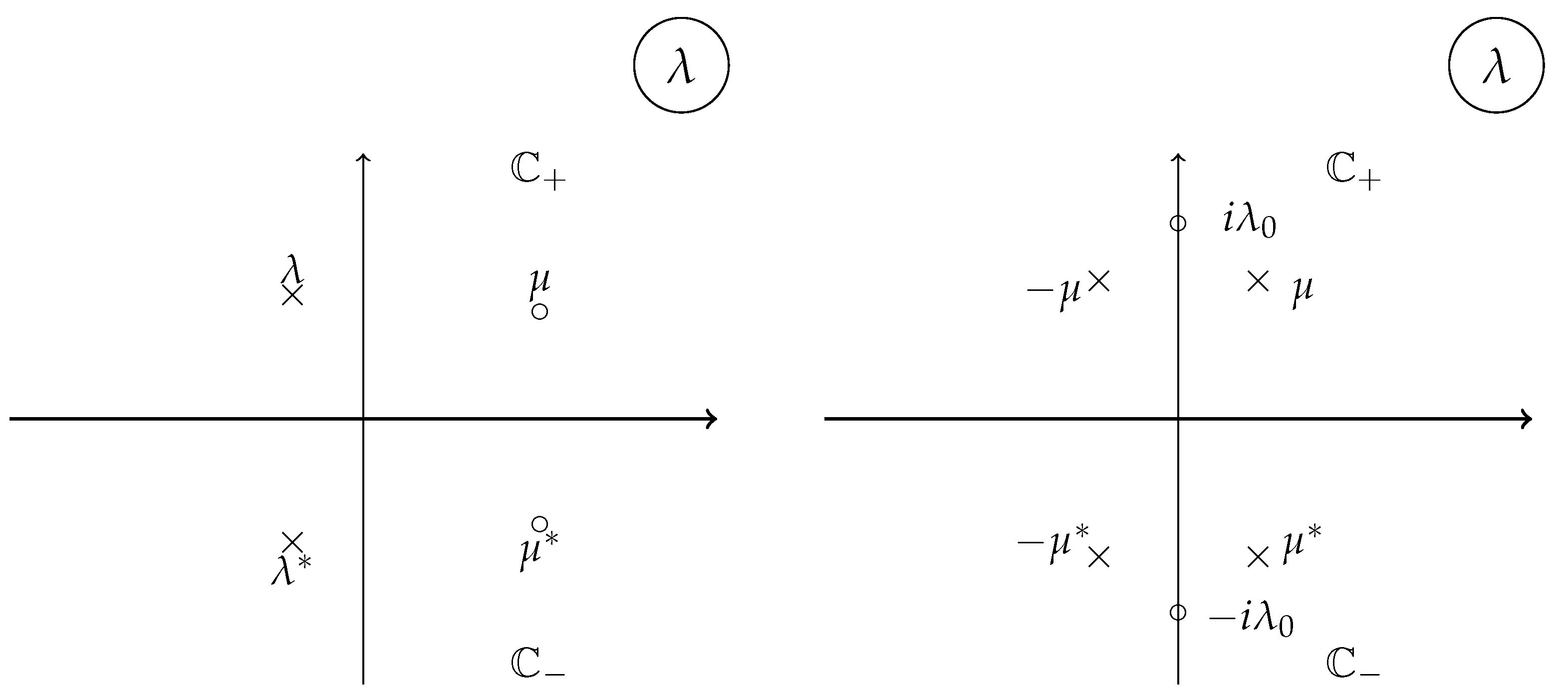
Remark 10. 

Let us assume that the zeroes and the pole singularities of ${\xi }^{+}(x,t,\lambda )$ (resp. ${\xi }^{-}(x,t,\lambda )$) are located at the points ${\lambda }_j^{+}\in {\mathbb{Q}}_1\cup {\mathbb{Q}}_3$ (resp. at ${\lambda }_j^{-}\in {\mathbb{Q}}_2\cup {\mathbb{Q}}_4$). Taking into account the symmetries of the FAS (89) we conclude that:

 1. 

if ${\lambda }_j^{+}$ is a zero or pole of ${\xi }^{+}(x,t,\lambda )$, then there must exist ${\lambda }_p^{+}=-{\lambda }_j^{+}$, which is also a zero or pole of ${\xi }^{+}(x,t,\lambda )$;

 2. 

if ${\lambda }_j^{-}$ is a zero or pole of ${\xi }^{-}(x,t,\lambda )$, then there must exist ${\lambda }_p^{-}=-{\lambda }_j^{-}$, which is also zero or pole of ${\xi }^{-}(x,t,\lambda )$.

 3. 

if ${\lambda }_j^{+}$ is a zero or pole of ${\xi }^{+}(x,t,\lambda )$, then there must exist ${\lambda }_p^{-}={\left({\lambda }_j^{+}\right)}^{\ast }$ which is a zero or pole of ${\xi }^{-}(x,t,\lambda )$.

Choosing proper enumeration of the zeroes and poles we can arrange them so that ${\lambda }_j^{+}\in {\mathbb{Q}}_1$, $j=1,\dots ,N$, ${\lambda }_{j+N}^{+}=-{\lambda }_j^{+}\in {\mathbb{Q}}_3$, $j=1,\dots ,N$, ${\lambda }_j^{-}={\left({\lambda }_j^{+}\right)}^{\ast }\in {\mathbb{Q}}_4$, $j=1,\dots ,N$ and ${\lambda }_{j+N}^{-}={\left({\lambda }_{j+N}^{+}\right)}^{\ast }\in {\mathbb{Q}}_2$, $j=1,\dots ,N$.

The FAS of $L\left(\lambda \right)$, which are related to the solution of the RHP by ${\chi }^{\pm }(x,\lambda )={\xi }^{\pm }(x,\lambda )e^{I{\lambda }^{2}Jx}$ allow one to construct the resolvent of the operator L and then to investigate its spectral properties. By resolvent of $L\left(\lambda \right)$ we understand the integral operator $R\left(\lambda \right)$ with kernel $R(x,y,\lambda )$, which satisfies

$$L\left(\lambda \right)\left(R\right(\lambda \left)f\right)\left(x\right)=f\left(x\right),$$

(270)

where $f\left(x\right)$ is an n-component vector function in ${\mathbb{C}}^n$ with bounded norm, i.e., ${\int }_{-\infty }^{\infty }dy\left(f^{†}\left(y\right)f\left(y\right)\right)<\infty$.

From the general theory of linear operators [79,80] we know that the point $\lambda$ in the complex $\lambda$-plane is a regular point if $R\left(\lambda \right)$ is the kernel of a bounded integral operator. In each connected subset of regular points, $R\left(\lambda \right)$ must be analytic in $\lambda$.

The points $\lambda$ which are not regular constitute the spectrum of $L\left(\lambda \right)$. Roughly speaking the spectrum of $L\left(\lambda \right)$ consist of two types of points:

• (i) the continuous spectrum of $L\left(\lambda \right)$ consists of all points $\lambda$ for which $R\left(\lambda \right)$ is an unbounded integral operator;
• (ii) the discrete spectrum of $L\left(\lambda \right)$ consists of all points $\lambda$ for which $R\left(\lambda \right)$ develops pole singularities.

Let us now show how the resolvent $R\left(\lambda \right)$ can be expressed through the FAS of $L\left(\lambda \right)$. Here and below, we will limit ourselves with Lax operators L which are quadratic pencils of $\lambda$ and have the form (78) (i.e., $N_1=2$). Assuming that the eigenvalues of J are different and real we can always order them so that

$$\begin{array}{c}\hfill J=\mathrm{diag}(a_1,a_2,\cdots ,a_n),a_1>a_2>\dots a_k>0>a_{k+1}>\dots >a_n\end{array}$$

(271)

In Section 2 above, we constructed the FAS of such operators. Using them we can write down $R\left(\lambda \right)$ in the form:

$$R\left(\lambda \right)f\left(x\right)={\int }_{-\infty }^{\infty }R(x,y,\lambda )f\left(y\right),$$

(272)

the kernel $R(x,y,\lambda )$ of the resolvent is given by:

$$R(x,y,\lambda )=\left\{\begin{array}{cc}{R}^{+}(x,y,\lambda )\hfill & for\lambda \in {\mathbb{Q}}_1\cup {\mathbb{Q}}_3,\hfill \\ R^{-}(x,y,\lambda )\hfill & for\lambda \in {\mathbb{Q}}_2\cup {\mathbb{Q}}_4,\hfill \end{array}\right.$$

(273)

where

$$\begin{array}{ccc}\hfill R^{\pm }(x,y,\lambda )& =& \pm i{\chi }^{\pm }(x,\lambda ){\Theta }^{\pm }(x-y){\widehat{\chi }}^{\pm }(y,\lambda ),\hfill \\ \hfill {\Theta }^{\pm }\left(z\right)& =& \theta (\mp z){\Pi }_0-\theta (\pm z)(11-{\Pi }_0),{\Pi }_0=\sum _{s=1}^{k_0}{E}_{ss},\hfill \end{array}$$

(274)

where $k_0$ is the number of positive eigenvalues of J, see (271). Due to the condition $trJ={\sum }_{s=1}^n{a}_s=0$, $k_0$ is fixed up uniquely.

The next theorem establishes that $R(x,y,\lambda )$ is indeed the kernel of the resolvent of $L\left(\lambda \right)$.

Theorem 3. 

Let $\mathcal{Q}(x,t,\lambda )$ satisfy conditions (C.1) and (C.2) and let ${\lambda }_j^{\pm }$ be the simple zeroes of the solutions ${\xi }^{\pm }(x,t,\lambda )$ of the RHP. Let ${\chi }^{\pm }(x,\lambda )={\xi }^{\pm }(x,\lambda )exp\left(i{\lambda }^{2}Jx\right)$ and let $R^{\pm }(x,y,\lambda )$ be defined as in Equation (274). Then:

 1. 

${\chi }^{\pm }(x,\lambda )$ will be FAS of a quadratic pencil of the form (86) whose coefficients will be expressed through $Q_s(x,t)$ as in (87).

 2. 

$R^{\pm }(x,y,\lambda )$ is a kernel of a bounded integral operator for $Im{\lambda }^2\ne 0$;

 3. 

$R(x,y,\lambda )$ is uniformly bounded function for ${\lambda }^2\in \mathbb{R}$ and provides a kernel of an unbounded integral operator;

 4. 

$R^{\pm }(x,y,\lambda )$ satisfy the equation:

$$L\left(\lambda \right)R^{\pm }(x,y,\lambda )=11\delta (x-y).$$

(275)

Idea of the proof. 

1.

is obvious from the fact that ${\chi }^{\pm }(x,\lambda )$ are the FAS of $L\left(\lambda \right)$ (86). It is also easy to see that if $\mathcal{Q}(x,t,\lambda )$ satisfies conditions (C.1) and (C.2) then $U_2(x,t)$ and $U_1(x,t)$ will also satisfy condition C1. In addition obviously ${\chi }^{\pm }(x,\lambda )$ will satisfy condition C2 and will have poles and zeroes at the points ${\lambda }_j^{\pm }$, see Remark 10.

2.

Assume that $\mathrm{Im}{\lambda }^2>0$ and consider the asymptotic behavior of $R^{+}(x,y,\lambda )$ for $x,y\to \infty$. From Equation (86) we find that

$$\begin{array}{cc}\hfill R_{ij}^{+}(x,y,\lambda )& =\sum _{p=1}^n{\xi }_{ip}^{+}(x,\lambda )e^{-i{\lambda }^2{a}_p(x-y)}{\Theta }_{pp}^{+}(x-y){\widehat{\xi }}_{pj}^{+}(y,\lambda )\hfill \end{array}$$

(276)

We use the fact that ${\chi }^{+}(x,\lambda )$ has triangular asymptotics for $x\to \infty$ and ${\lambda }^2\in {\mathbb{C}}_{+}$ (see Equation (42)). With the choice of ${\Theta }^{+}(x-y)$ (274) we check that the right-hand side of (276) falls off exponentially for $x\to \infty$ and arbitrary choice of y. All other possibilities are treated analogously.

3.

For $\lambda \in \mathbb{R}\cup i\mathbb{R}$ the arguments of (2) can not be applied because the exponentials in the right-hand side of (276) $Im\lambda =0$ only oscillate. Thus, we conclude that $R^{\pm }(x,y,\lambda )$ for $\lambda \in \mathbb{R}$ is only a bounded function of x and thus the corresponding operator $R\left(\lambda \right)$ is an unbounded integral operator.

4.

The proof of Equation (275) follows from the fact that $L\left(\lambda \right){\chi }^{+}(x,\lambda )=0$ and

$$\frac{d{\Theta }^{\pm }(x-y)}{dx}=\mp 11\delta (x-y).$$

(277)

□

If the algebra $\mathfrak{g}\simeq sl\left(n\right)$ then ${\chi }^{+}(x,\lambda )$ and its inverse ${\widehat{\chi }}^{+}(x,\lambda )$ do not have common poles. In this case, condition C2 is valid also for $R^{+}(x,y,\lambda )$. However, this is not true for the orthogonal or symplectic algebras; in this case, $R^{+}(x,y,\lambda )$ may have poles of second order, which require additional care.

Now, we can derive the completeness relation for the eigenfunctions of the Lax operator L by applying the contour integration method (see, e.g., [23,81,82]) to the integral:

$$\mathcal{J}(x,y)=\frac{1}{2\pi i}{\oint }_{{\gamma }_1\cup {\gamma }_3}d\lambda \lambda R^{+}(x,y,\lambda )-\frac{1}{2\pi i}{\oint }_{{\gamma }_2\cup {\gamma }_4}d\lambda \lambda R^{-}(x,y,\lambda ),$$

(278)

where the contours ${\gamma }_j$ are shown on the Figure 10. The idea is to calculate $\mathcal{J}(x,y)$ first using the Cauchy residue theorem. Taking into account that the contours ${\gamma }_1$ and ${\gamma }_3$ are positively oriented, while ${\gamma }_2$ and ${\gamma }_4$ are negatively oriented we obtain:

$$\begin{array}{cc}\hfill & \mathcal{J}(x,y)\hfill \\ \hfill & =\sum _{j=1}^N\left(\underset{\lambda ={\lambda }_j^{+}}{Res}\lambda R^{+}(x,y,\lambda )+\underset{\lambda =-{\lambda }_j^{+}}{Res}\lambda R^{+}(x,y,\lambda )-\underset{\lambda ={\lambda }_j^{-}}{Res}\lambda R^{-}(x,y,\lambda )-\underset{\lambda =-{\lambda }_j^{-}}{Res}\lambda R^{-}(x,y,\lambda )\right).\hfill \end{array}$$

(279)

We can also evaluate $\mathcal{J}(x,y)$ integrating along the contours. The integration along the real and purely imaginary axis provides the contribution coming from the continuous spectrum of L. The integration along the infinite arcs of the contours can be evaluated explicitly. To this end, we use the fact that ${\xi }^{\pm }(x,\lambda )$ are canonically normalized we find:

$$\begin{array}{cc}\hfill {\mathcal{J}}_{\infty }^{+}(x,y)& =\frac{1}{2\pi i}{\oint }_{{\gamma }_{1,\infty }\cup {\gamma }_{3,\infty }}d\lambda \lambda R^{+}(x,y,\lambda )=\frac{1}{4\pi i}{\oint }_{{\gamma }_{1,\infty }\cup {\gamma }_{3,\infty }}d{\lambda }^2{e}^{-i{\lambda }^{2}J(x-y)}{\Theta }^{+}(x-y)\hfill \\ \hfill & =\frac{1}{4\pi i}{\int }_{-\infty }^{\infty }d{\lambda }^2{e}^{-i{\lambda }^{2}J(x-y)}{\Theta }^{+}(x-y)\hfill \end{array}$$

(280)

$$\begin{array}{cc}\hfill {\mathcal{J}}_{\infty }^{-}(x,y)& =\frac{1}{2\pi i}{\oint }_{{\gamma }_{2,\infty }\cup {\gamma }_{4,\infty }}d\lambda \lambda R^{-}(x,y,\lambda )=\frac{1}{4\pi i}{\oint }_{{\gamma }_{2,\infty }\cup {\gamma }_{4,\infty }}d{\lambda }^2{e}^{-i{\lambda }^{2}J(x-y)}{\Theta }^{-}(x-y)\hfill \\ \hfill & =-\frac{1}{4\pi i}{\int }_{-\infty }^{\infty }d{\lambda }^2{e}^{-i{\lambda }^{2}J(x-y)}{\Theta }^{-}(x-y).\hfill \end{array}$$

(281)

Adding these two answers and using the definitions of ${\Theta }^{\pm }(x-y)$ we find

$$\begin{array}{c}\hfill {\mathcal{J}}_{\infty }^{+}(x,y)+{\mathcal{J}}_{\infty }^{-}(x,y)=\frac{1}{4\pi i}{\int }_{-\infty }^{\infty }d{\lambda }^2{e}^{-i{\lambda }^2(x-y)}11=\frac{1}{2}\delta (x-y)\sum _{s=1}^n\frac{1}{a_s}{E}_{ss}.\end{array}$$

(282)

Equating the two answers for $\mathcal{J}(x,y)$ we find the following completeness relations for the FAS of L:

$$\begin{array}{c}\delta (x-y)\frac{1}{2}\sum _{s=1}^n\frac{1}{a_s}{E}_{ss}=\frac{1}{2\pi }{\int }_{-\infty }^{\infty }d{\lambda }^2\left\{\sum _{s=1}^{k_0}|{\chi }^{\left[s\right]+}(x,\lambda )\rangle \langle {\widehat{\chi }}^{\left[s\right]+}(y,\lambda )|-\sum _{s=k_0+1}^n|{\chi }^{\left[s\right]-}(x,\lambda )\rangle \langle {\widehat{\chi }}^{\left[s\right]-}(y,\lambda )|\right\}\hfill \\ \hfill +\sum _{j=1}^N\left(\underset{\lambda ={\lambda }_j^{+}}{\mathrm{Res}}\lambda R^{+}(x,y,\lambda )+\underset{\lambda =-{\lambda }_j^{+}}{\mathrm{Res}}\lambda R^{+}(x,y,\lambda )-\underset{\lambda ={\lambda }_j^{-}}{\mathrm{Res}}\lambda R^{-}(x,y,\lambda )-\underset{\lambda =-{\lambda }_j^{-}}{\mathrm{Res}}\lambda R^{-}(x,y,\lambda )\right).\end{array}$$

(283)

This relation (283) allows one to expand any vector-function $|z\left(x\right)\rangle \in {\mathbb{C}}^n$ over the eigenfunctions of the system (86). If we multiply (283) on the right by $J\mid z\left(y\right)\rangle$ and integrate over y we obtain:

$$\begin{array}{cc}\hfill \mid z\left(x\right)\rangle & =\frac{i}{2\pi }{\int }_{-\infty }^{\infty }d\lambda \left\{{\sum }_{s=1}^{k_0}|{\chi }^{\left[s\right]+}(x,\lambda )\rangle ·{\zeta }_s^{+}\left(\lambda \right)-{\sum }_{s=k_0+1}^n{\chi }^{\left[s\right]-}(x,\lambda )\rangle ·{\zeta }_s^{-}\left(\lambda \right)\right\}\\ & +{\sum }_{j=1}^N{\nu }_j\left(\left|{\mathbf{n}}_j^{+}\left(x\right)\right.〉{\zeta }_j^{+}-\left|{\mathbf{n}}_j^{-}\left(x\right)\right.〉{\zeta }_j^{-}\right),\end{array}$$

(284)

where the expansion coefficients are of the form:

$$\begin{array}{cc}\hfill {\zeta }_s^{\pm }\left(\lambda \right)& =-i{\int }_{-\infty }^{\infty }dx\langle {\widehat{\chi }}^{\left[s\right]\pm }(x,\lambda )|J|z\left(x\right)\rangle ,{\zeta }_j^{\pm }\left(\lambda \right)=-i{\int }_{-\infty }^{\infty }dx\left.〈{\mathbf{m}}_j^{\pm }\right|J\left|z\left(x\right)\right.〉.\hfill \end{array}$$

(285)

Corollary 3. 

The discrete spectrum of the Lax operator (86) consists of the poles of the resolvent $R^{\pm }(x,y,\lambda )$, which are described in Remark 10.

Remark 11. 

Here, we used also the fact that all eigenvalues of J are non-vanishing. In the case when one (or several) of them vanishes, we can prove the completeness of the eigenfunctions only on the image of ${ad}_J$, which is a subspace of ${\mathbb{C}}^n$.

Remark 12. 

The authors are aware that these type of derivations need additional arguments to be made rigorous. One of the real difficulties is to find explicit conditions on the potentials $U_2\left(x\right)$ and $U_1\left(x\right)$ that are equivalent to the condition (C.2). Nevertheless, there are situations (e.g., the reflectionless potentials) when all these conditions are fulfilled and all eigenfunctions of $L\left(\lambda \right)$ can be explicitly calculated. Another advantage of this approach is the possibility to apply it to Lax operators with more general dependence on λ, e.g., polynomial and rational.

11. Natural Generalizations

We outline possible natural generalizations of the above method. Thus, we demonstrate that with our method we can treat a number of new classes of Lax pairs. Treating the quadratic pencil we started by constructing the FAS. We did that to demonstrate that the FAS exist also for pencils of higher order. In fact, since we are dealing with RHP means that the FAS of the Lax pair are directly related to the solution of the RHP, see Equation (290) below.

11.1. Cubic Pencils as Lax Operators

Assume that

$$\begin{array}{cc}\hfill L& \equiv i\frac{\partial \psi }{\partial x}+(U_3+\lambda U_2+{\lambda }^2{U}_1-{\lambda }^{3}J)\psi (x,t,\lambda )=0,\hfill \\ \hfill M& \equiv i\frac{\partial \psi }{\partial t}+(V_3+\lambda V_2+{\lambda }^2{V}_1-{\lambda }^{3}K)\psi (x,t,\lambda )=0,\hfill \end{array}$$

(286)

where J and K are diagonal matrices with real eigenvalues. If we assume $U_k$ and $V_k$ to be generic elements of the Lie algebra $\mathfrak{g}$ the corresponding NLEE will be a system of $3N_g$ equations, where $N_g=dim\mathfrak{g}$. In order to avoid this difficulty, we introduce the automorphism C of the algebra of third order, i.e., $C^3=11$. For simplicity we can take it in the form:

$$\begin{array}{c}\hfill C\left(X\right)\equiv C^{-1}XC,C=\left(\begin{array}{ccc}11& 0& 0\\ 0& {\omega }^{2}11& 0\\ 0& 0& \omega 11\end{array}\right),\omega =exp(2\pi i/3).\end{array}$$

(287)

Using it we will introduce a grading of $\mathfrak{g}$

$$\begin{array}{cc}\hfill \mathfrak{g}& ={\mathfrak{g}}^{\left(0\right)}\cup {\mathfrak{g}}^{\left(1\right)}\cup {\mathfrak{g}}^{\left(2\right)},X_{\left(k\right)}\in {\mathfrak{g}}^{\left(k\right)},X_{\left(0\right)}=\left(\begin{array}{ccc}{X}_{(0;1)}& 0& 0\\ 0& X_{(0;2)}& 0\\ 0& 0& X_{(0;3)}\end{array}\right),\hfill \\ \hfill X_{\left(1\right)}& =\left(\begin{array}{ccc}0& 0& X_{(1;1)}\\ X_{(1;2)}& 0& 0\\ 0& X_{(1;3)}& 0\end{array}\right),X_{\left(2\right)}=\left(\begin{array}{ccc}0& X_{(2;1)}& 0\\ 0& 0& X_{(2;2)}\\ X_{(2;3)}& 0& 0\end{array}\right).\hfill \end{array}$$

(288)

Of course $U_3$, J and K are elements of ${\mathfrak{g}}^{\left(0\right)}$.

The RHP is formulated as:

$$\begin{array}{cc}\hfill {\xi }^{+}(x,t,\lambda )& ={\xi }^{-}(x,t,\lambda )G_k(x,t,\lambda ),\lambda \in l_k,\hfill \\ \hfill i\frac{\partial G}{\partial x}& ={\lambda }^3[J,G_k(x,t,\lambda )],i\frac{\partial G}{\partial x}={\lambda }^3[K,G_k(x,t,\lambda )].\hfill \end{array}$$

(289)

${\xi }^{+}(x,t,\lambda )$ is analytic in the sectors ${\Omega }_0\cup {\Omega }_2\cup {\Omega }_4$ while ${\xi }^{-}(x,t,\lambda )$ is analytic in the sectors ${\Omega }_1\cup {\Omega }_3\cup {\Omega }_5$, see the left panel of Figure 3. The FAS of the Lax pair (286) are given by:

$$\begin{array}{c}\hfill {\chi }^{\pm }(x,t,\lambda )={\xi }^{+}(x,t,\lambda )exp\left(i{\lambda }^3(Jx+Kt)\right).\end{array}$$

(290)

The parametrization of the RHP will be given by (compare with Equations (167) and (174)):

$$\begin{array}{cc}\hfill {\xi }^{\pm }(x,t,\lambda )& =exp\left(\mathcal{Q}(x,t,\lambda )\right),\mathcal{Q}(x,t,\lambda )=\sum _{s=1}^{\infty }{\lambda }^{-s}{Q}_s(x,t),\hfill \\ \hfill C^{-1}\mathcal{Q}(x,t,\lambda )C& =\mathcal{Q}(x,t,\omega \lambda ),i.e.,C^{-1}{Q}_s(x,t)C={\omega }^{-s}{Q}_s(x,t)\in {\mathfrak{g}}^{(3-k(s\left)\right)}\hfill \end{array}$$

(291)

where $k\left(s\right)=s(mod3)$. The contour of the corresponding RHP consists of the rays $l_k$, $k=0,\dots 5$ (see the left panel of Figure 3).

Using Equations (78)–(80) we obtain the following parametrization of the Lax pair (286):

$$\begin{array}{cc}\hfill U_1& ={\mathrm{ad}}_J{Q}_1,U_2={\mathrm{ad}}_J{Q}_2+\frac{1}{2}{\mathrm{ad}}_{Q_1}{U}_1,\hfill \\ \hfill U_3& =\frac{1}{2}\left({\mathrm{ad}}_{Q_1}{\mathrm{ad}}_J{Q}_2+{\mathrm{ad}}_{Q_2}{\mathrm{ad}}_J{Q}_1\right)+\frac{1}{6}{\mathrm{ad}}_{Q_1}^2{U}_1+{\mathrm{ad}}_J{Q}_3,\hfill \\ \hfill V_1& ={\mathrm{ad}}_K{Q}_1,V_2={\mathrm{ad}}_K{Q}_2+\frac{1}{2}{\mathrm{ad}}_{Q_1}{V}_1,\hfill \\ \hfill V_3& =\frac{1}{2}\left({\mathrm{ad}}_{Q_1}{\mathrm{ad}}_K{Q}_2+{\mathrm{ad}}_{Q_2}{\mathrm{ad}}_K{Q}_1\right)+\frac{1}{6}{\mathrm{ad}}_{Q_1}^2{V}_1+{\mathrm{ad}}_K{Q}_3.\hfill \end{array}$$

(292)

The rest of the calculations follow the same ideas as developed above.

11.2. Cubic Pencils with Dihedral Reduction Group

Let us now demonstrate another class of cubic pencils possessing additional symmetry. To this end, we start with the pencil (286) and apply to it additional ${\mathbb{Z}}_2$-reduction such that, see [49]:

$$\begin{array}{cc}\hfill \mathcal{L}& \equiv i\frac{\partial \psi }{\partial x}+\left(U(x,t,\lambda )+R_0{U}^{\ast }(x,t,1/{\lambda }^{\ast })R_0^{-1}\right)\psi (x,t,\lambda )=0,\hfill \\ \hfill \mathcal{M}& \equiv i\frac{\partial \psi }{\partial x}+\left(V(x,t,\lambda )+R_0{V}^{\ast }(x,t,1/{\lambda }^{\ast })R_0^{-1}\right)\psi (x,t,\lambda )=0,\hfill \\ \hfill U(x,t,\lambda )& =U_3+\lambda U_2+{\lambda }^2{U}_1-{\lambda }^{3}J,V(x,t,\lambda )=V_3+\lambda V_2+{\lambda }^2{V}_1-{\lambda }^{3}K,\hfill \end{array}$$

(293)

where $R_0$ must be constant matrix satisfying $R_0^2=11.$ With this additional reduction the grading of the algebra

$$\begin{array}{cc}\hfill \mathfrak{g}& ={\mathfrak{g}}^{\left(0\right)}\cup {\mathfrak{g}}^{\left(1\right)}\cup {\mathfrak{g}}^{\left(2\right)}\cup {\widehat{\mathfrak{g}}}^{\left(0\right)}\cup {\widehat{\mathfrak{g}}}^{\left(1\right)}\cup {\widehat{\mathfrak{g}}}^{\left(2\right)},\hfill \end{array}$$

(294)

where the elements $X_{\left(k\right)}\in {\mathfrak{g}}^{\left(k\right)}$ were described above in (288) while ${\widehat{\mathfrak{g}}}^{\left(k\right)}$ consist of the elements $R_0{X}_{\left(k\right)}^{\ast }{R}_0^{-1}$.

The RHP now is formulated on a different contour $\Gamma \equiv {\cup }_{k=0}^5{l}_k\cup {\mathbb{S}}^1$, where ${\mathbb{S}}^1$ is the unit circle, see the right panel of Figure 3. For the formulation of the RHP we need to introduce the besides rays $l_k$, also the arcs $l_{\alpha }$ of the unit circle:

$$\begin{array}{cc}\hfill l_k& \equiv arg\lambda =\frac{k\pi }{3},|\lambda |\ge 1;l_{k+6}\equiv arg\lambda =\frac{k\pi }{3},|\lambda |\le 1;\hfill \\ \hfill l_{\alpha }& \equiv |\lambda |=1,arg\lambda \le \frac{(\alpha -1)\pi }{3}\le \frac{\alpha \pi }{3}.\hfill \end{array}$$

(295)

Then, we have:

$$\begin{array}{cc}\hfill {\xi }_k^{+}(x,t,\lambda )& ={\xi }_k^{-}(x,t,\lambda )G_k(x,t,\lambda ),\lambda \in l_k,\hfill \\ \hfill {\xi }_{k+6}^{+}(x,t,\lambda )& ={\xi }_{k+6}^{-}(x,t,\lambda )R_0{G}_k^{\ast }(x,t,1/{\lambda }^{\ast })R_0^{-1},\lambda \in l_{k+6},\hfill \\ \hfill {\xi }_{\alpha +6}^{\pm }(x,t,\lambda )& ={\xi }_{\alpha }^{\pm }(x,t,\lambda )G_{\alpha }(x,t,\lambda ),\lambda \in l_{\alpha },\hfill \\ \hfill i\frac{\partial G}{\partial x}& ={\lambda }^3[J,G_k(x,t,\lambda )],i\frac{\partial G}{\partial x}={\lambda }^3[K,G_k(x,t,\lambda )].\hfill \end{array}$$

(296)

The FAS of the Lax pair (293) in each of the sectors ${\Omega }_k$, $k=0,\dots ,11$ (see right panel of Figure 3), is related to the solutions of the RHP (296) as follows:

$$\begin{array}{c}\hfill {\chi }_k^{\pm }(x,t,\lambda )={\xi }_k^{\pm }(x,t,\lambda )exp\left(i{\lambda }^3(Jx+Kt)\right).\end{array}$$

(297)

For the RHP (296), we have to use different parametrizations inside and outside of the unit circle ${\mathbb{S}}^1$. Outside the unit circle we will have the parametrization (291). Now, we must have:

$$\begin{array}{cccc}\hfill {\xi }^{\pm }(x,t,\lambda )=exp\left(\mathcal{Q}(x,t,\lambda )\right),& \mathcal{Q}(x,t,\lambda )=\sum _{s=1}^{\infty }{\lambda }^{-s}{Q}_s(x,t),\hfill & \hfill |\lambda |& \ge 1;\hfill \\ \hfill {\xi }^{\pm }(x,t,\lambda )=R_0{\xi }^{\mp }(x,t,1/{\lambda }^{\ast })R_0^{-1}& =exp\left(R_0{\mathcal{Q}}^{\ast }(x,t,1/{\lambda }^{\ast })R_0^{-1}\right),\hfill \\ \hfill R_0{\mathcal{Q}}^{\ast }(x,t,1/{\lambda }^{\ast })R_0^{-1}& =\sum _{s=1}^{\infty }{\lambda }^s{R}_0{Q}_s^{\ast }(x,t)R_0^{-1},\hfill & \hfill |\lambda |& \le 1;\hfill \end{array}$$

(298)

Then, the parametrization of $\mathcal{L}$ and $\mathcal{M}$ is given by (293).

It allows one to derive new types of integrable NLEE. The derivation of their soliton solutions consists in straightforward execution of the dressing method.

12. Discussion and Conclusions

Our intention was to review some of the old papers which were milestones in the past, but for various reasons tend to be forgotten. Another motivation for this paper was our intention to generalize these results for quadratic pencils and pencils of higher degrees.

Of course, many of the results we mentioned here were first introduced for the GZS system. One of the important results is the resolvent for the Lax operator L [15,83,84] expressed in terms of the FAS. Combined with the contour integration method, it allows one to construct the spectral decompositions of L. They also allow one to prove that the poles and zeroes of FAS provide the discrete eigenvalues of L. Rigorous proofs would hardly be possible with these methods, but their importance is in the fact that they can be applied to wide class of non-self-adjoint Lax operators.

In the Introduction, we already listed a number of results about the interpretation of the ISM as GFT and ISM for the GZS systems. Our comment on it is that this idea can also be generalized for the quadratic pencils considered as Lax operators above. We intend to continue the idea in our future publications. Of course, there will be specifics for the homogeneous and symmetric spaces.

The initial ideas that we have extended above for quadratic pencils have been developed before by other influential scientists, see some of theirs reviews and monographs [10,12,15,30,84,85,86,87,88,89]. It is important to note that these ideas are also applicable to discrete evolution equations as Ablowitz-Ladik system [90,91].

Another important approach to integrable NLEE has been developed by Shabat, Mikhailov, Yamilov, Svinolupov et al., see [88,92,93,94]. This allows one to derive systems of equations that possess higher symmetries, or higher integrals of motion. Lately, this method has been used by Zhao [94], who covered all integrable systems in two independent functions. Some of these equations were shown to possess Lax representations related to the twisted Kac-Moody algebras [95].

Special attention must be paid to the NLEE with deep Mikhailov reduction groups, like ${\mathbb{Z}}_h$ and ${\mathbb{D}}_h$. Typically, by h we denote the Coxeter number of the corresponding simple Lie algebra. Here, we include the families of KdV and MKdV eqs., as well as 2-dimensional Toda field theories [96,97,98,99,100,101,102,103,104,105] as well as some Camassa–Holm type equations [106,107,108,109,110,111,112].

The Kulish–Sklyanin system, or in other words the 3-component NLS related to the BD.I symmetric space has important applications to the spin-1 Bose–Einstein condensate, see [25,78,113,114,115,116,117,118,119,120,121,122,123,124,125,126,127]. Using the dressing method in [115,128], we calculated the limit of the dressing factor for $t\to \pm \infty$. This allowed us to describe the soliton interactions, i.e., to calculate the center-of-mass and the phase shifts in the soliton interactions.

In short, we illustrated on the class of quadratic pencils how our method works. However, we could apply it to pencils of higher order, see Section 11 where we outlined how one could approach cubic pencils. The straightforward generalization to pencils of higher order meets with a difficulty: the corresponding NLEE should involve too many independent variables. We avoided this difficulty by choosing the parametrization of the RHP. Generic parametrization like (76) should involve generic choice for $Q_s(x,t)$. However, we imposed on $\mathcal{Q}(x,t,\lambda )$ Mikhailov reduction. In particular, for the case of symmetric spaces we chose $Q_s(x,t)\in {\mathfrak{g}}^{\left(1\right)}$, see Equation (187). Similar ideas could be generalized also to cubic and higher order pencils.

Finally, in Section 11, we demonstrated how our approach could be combined with additional Mikhailov reductions, which may modify the RHP. Applying such reductions changes the contour of the RHP, which in turn requires us to use different parametrization outside and inside the unit circle, see Equation (298).

In our final remarks, we mention the generalizations to $2+1$ dimensions [29,129,130,131], the MNLS related to spectral curves [106,132,133,134,135,136,137] and the hierarchies of Hamiltonian structures. It is known that one can relate Poisson brackets on the quadratic pencils which, along with the integrals of motion, allow one to interpret the NLEE in the hierarchy as Hamiltonian equations of motion. Such Poisson brackets have been introduced for the $sl\left(2\right)$ polynomial pencils by Kulish and Reyman [36]. Of course, they allow generalization to any semi-simple Lie algebra. We already mentioned that for the generalized Zakharov–Shabat systems this has been already performed. In fact, the spectral theory of the recursion operators has been constructed which generate all NLEE along with its Hamilton formulation. For the quadratic pencils, the recursion operators have not yet been constructed; we hope that this problem will be solved soon.

References

1. Zakharov, V.E.; Faddeev, L.D. Korteweg-de Vries equation: A completely integrable Hamiltonian system. Funct. Anal. Appl. 1971, 5, 280–287. [Google Scholar] [CrossRef]
2. Zabusky, N.J. Fermi–Pasta–Ulam, solitons and the fabric of nonlinear and computational science: History, synergetics, and visiometrics. Chaos 2005, 15, 015102. [Google Scholar] [CrossRef]
3. Zakharov, V.E.; Shabat, A.B. Exact theory of two-dimensional self-focusing and one-dimensional self-modulation of waves in nonlinear media. Sov. Phys. JETP 1972, 34, 62–69. [Google Scholar]
4. Zakharov, V.E.; Shabat, A.B. Interaction between solitons in a stable medium. Sov. Phys. JETP 1973, 37, 823–828. [Google Scholar]
5. Wadati, M. The exact solution of the modified Korteweg de Vries equation. J. Phys. Soc. Jpn. 1972, 32, 1681. [Google Scholar] [CrossRef]
6. Zakharov, V.E.; Manakov, S.V. On the theory of resonance interactions of wave packets in nonlinear media. Zh. Exp. Teor. Fiz 1975, 69, 1654–1673. [Google Scholar]
7. Manakov, S.V. On the theory of two-dimensional stationary self-focusing of electromagnetic waves. Sov. Phys. JETP 1974, 38, 248. [Google Scholar]
8. Ablowitz, A.; Clarkson, A. Solitons, Nonlinear Evolution Equations and Inverse Scattering; Cambridge University Press: Cambridge, UK, 1991. [Google Scholar]
9. Calogero, F.; Degasperis, A. Spectral transform and solitons. I. In Studies in Mathematics and its Applications; Elsevier: Haarlem, The Netherlands, 1982; Volume 13. [Google Scholar]
10. Faddeev, L.D.; Takhtadjan, L.A. Hamiltonian Methods in the Theory of Solitons; Springer: Berlin/Heidelberg, Germany, 1987. [Google Scholar]
11. Gerdjikov, V.S.; Yanovski, A.B. Completeness of the eigenfunctions for the Caudrey–Beals–Coifman system. J. Math. Phys. 1994, 35, 3687–3725. [Google Scholar] [CrossRef]
12. Novikov, S.; Manakov, S.; Pitaevskii, L.; Zakharov, V. Theory of Solitons: The Inverse Scattering Method; Plenum, Consultants Bureau: New York, NY, USA, 1984. [Google Scholar]
13. Shabat, A.B. A one-dimensional scattering theory. I. Differ. Uravn. 1972, 8, 164–178. [Google Scholar]
14. Shabat, A.B. The inverse scattering problem for a system of differential equations. Funkts. Anal. Prilozhen 1975, 9, 75–78. [Google Scholar] [CrossRef]
15. Gerdjikov, V.S. Algebraic and analytic aspects of n-wave type equations. Contemp. Math. 2002, 301, 35–68. [Google Scholar]
16. Zakharov, V.E.; Shabat, A.B. A scheme for integrating nonlinear evolution equations of mathematical physics by the inverse scattering method. I. Funkts. Anal. Prilozhen 1974, 8, 43–53. [Google Scholar]
17. Zakharov, V.E.; Shabat, A.B. Integration of the nonlinear equations of mathematical physics by the inverse scattering method. Funkts. Anal. Prilozhen 1979, 13, 13–22. [Google Scholar] [CrossRef]
18. Mikhailov, A.V. The reduction problem and the inverse scattering problem. Phys. D 1981, 3D, 73–117. [Google Scholar] [CrossRef]
19. Beals, R.; Coifman, R.R. Scattering and inverse scattering for first order systems. Commun. Pure Appl. Math. 1984, 37, 39. [Google Scholar] [CrossRef]
20. Gerdjikov, V.S.; Yanovski, A.B. CBC systems with Mikhailov reductions by Coxeter automorphism. I. Spectral theory of the recursion operators. Stud. Appl. Math. 2015, 134, 145–180. [Google Scholar] [CrossRef]
21. Helgasson, S. Differential Geometry, Lie Groups and Symmetric Spaces; Graduate Studies in Mathematics; AMS: Providence, RI, USA, 2012; Volume 34. [Google Scholar]
22. Gerdjikov, V.S. Generalised Fourier transforms for the soliton equations. gauge covariant formulation. Inverse Probl. 1986, 2, 51–74. [Google Scholar] [CrossRef]
23. Ablowitz, M.J.; Kaup, D.J.; Newell, A.C.; Segur, H. The inverse scattering transform—Fourier analysis for nonlinear problems. Stud. Appl. Math. 1974, 53, 249–315. [Google Scholar] [CrossRef]
24. Constantin, A.; Gerdjikov, V.S.; Ivanov, R.I. Generalized Fourier transform for the Camassa–Holm equation. Inverse Probl. 2007, 23, 1565–1597. [Google Scholar] [CrossRef]
25. Gaiarin, S.; Perego, A.M.; da Silva, E.P.; Da Ros, F.; Zibar, D. Dual-polarization nonlinear Fourier transform-based optical communication system. Optica 2018, 5, 263–270. [Google Scholar] [CrossRef]
26. Gerdjikov, V.S. On nonlocal models of Kulish–Sklyanin type and generalized Fourier transforms. In Advanced Computing in Industrial Mathematics. Studies in Computational Intelligence; Georgiev, K., Todorov, M., Georgiev, I., Eds.; Springer: Berlin/Heidelberg, Germany, 2017; Volume 681, pp. 37–52. [Google Scholar]
27. Gerdjikov, V.S.; Khristov, E.K. On the evolution equations solvable through the inverse scattering problem. I. The spectral theory. Bulg. J. Phys. 1979, 7, 28–41. [Google Scholar]
28. Gerdjikov, V.S.; Khristov, E.K. On the evolution equations solvable through the inverse scattering problem. II. Hamiltonian structures and Backlund transformations. Bulg. J. Phys. 1979, 7, 119–133. [Google Scholar]
29. Gerdjikov, V.S.; Smirnov, A.O.; Matveev, V.B. From generalized Fourier transforms to spectral curves for the Manakov hierarchy. I. Generalized Fourier transforms. Eur. Phys. J. Plus 2020, 135, 659. [Google Scholar] [CrossRef]
30. Gerdjikov, V.S.; Vilasi, G.; Yanovski, A.B. Integrable Hamiltonian Hierarchies: Spectral and Geometric Methods; Lecture Notes in Physics; Springer: Berlin/Heidelberg, Germany, 2008; Volume 748. [Google Scholar]
31. Goossens, J.V.; Yousefi, M.; Jaou, Y.; Haffermann, H. Polarization-division multiplexing based on the nonlinear Fourier transform. Opt. Express 2017, 25, 437–462. [Google Scholar] [CrossRef]
32. Kaup, D.J. Closure of the squared Zakharov–Shabat eigenstates. J. Math. Annal. Appl. 1976, 54, 849–864. [Google Scholar] [CrossRef]
33. Smirnov, A.O.; Gerdjikov, V.S.; Matveev, V.B. From generalized fourier transforms to spectral curves for the Manakov hierarchy. II. Spectral curves for the Manakov hierarchy. Eur. Phys. J. Plus 2020, 135, 561. [Google Scholar] [CrossRef]
34. Gerdzhikov, M.I.I.V.S.; Kulish, P.P. Quadratic bundle and nonlinear equations. Theor. Math. Phys. 1980, 44, 784–795. [Google Scholar] [CrossRef]
35. Kaup, D.J.; Newell, A.C. An exact solution for a derivative nonlinear Schrödinger equation. J. Math. Phys. 1978, 19, 798–801. [Google Scholar] [CrossRef]
36. Kulish, P.P.; Reiman, A.G. Hamiltonian structure of polynomial bundles. J. Sov. Math. 1985, 28, 505–513. [Google Scholar] [CrossRef]
37. Gerdjikov, V.S. Riemann–Hilbert problems with canonical normalization and families of commuting operators. Pliska Stud. Math. Bulgar. 2012, 21, 201–216. [Google Scholar]
38. Gerdjikov, V.S.; Stefanov, A.A. New types of two component NLS-type equations. Pliska Stud. Math. 2016, 26, 53–66. [Google Scholar]
39. Gerdjikov, V.S.; Stefanov, A.A. On an example of derivative nonlinear Schrödinger equation with D2 reduction. Pliska Stud. Math. 2019, 30, 99–108. [Google Scholar]
40. Gerdjikov, V.S.; Yanovski, A.B. Riemann–Hilbert problems, families of commuting operators and soliton equations. J. Phys. Conf. Ser. 2014, 482, 012017. [Google Scholar] [CrossRef]
41. Ivanov, R. On the dressing method for the generalised Zakharov–Shabat system. Nucl. Phys. B 2004, 694, 509–524. [Google Scholar] [CrossRef]
42. Mikhailov, A.V.; Zakharov, V.E. On the integrability of classical spinor models in two-dimensional space–time. Commun. Math. Phys. 1980, 74, 21–40. [Google Scholar]
43. Zakharov, V.E. The inverse scattering method. In Solitons; Bullough, R.K., Caudrey, P.J., Eds.; Springer: Berlin/Heidelberg, Germany, 1980; pp. 243–286. [Google Scholar]
44. Zakharov, V.E. Exact solutions of the problem of parametric interaction of wave packets. Dokl. Akad. Nauk SSSR 1976, 228, 1314–1316. [Google Scholar]
45. Fordy, A.P.; Kulish, P.P. Nonlinear Schrödinger equations and simple lie algebras. Commun. Math. Phys. 1983, 89, 427–443. [Google Scholar] [CrossRef]
46. Gerdjikov, V.S.; Grahovski, G.G. Multi-component NLS models on symmetric spaces: Spectral properties versus representations theory. Symmetry Integr. Geom. Methods Appl. 2010, 6, 44–73. [Google Scholar] [CrossRef]
47. Matveev, V.B.; Smirnov, A.O. AKNS hierarchy, MRW solutions, Pn breathers, and beyond. J. Math. Phys. 2018, 59, 091419. [Google Scholar] [CrossRef]
48. Gerdjikov, R.I.V.; Grahovski, G. On integrable wave interactions and Lax pairs on symmetric spaces. Wave Motion 2017, 71, 53–70. [Google Scholar] [CrossRef]
49. Gerdjikov, R.I.V.; Stefanov, A. Riemann–Hilbert problem, integrability and reductions. J. Geom. Mech. 2019, 11, 167–185. [Google Scholar] [CrossRef]
50. Valchev, T.I. On certain reductions of integrable equations on symmetric spaces. AIP Conf. Proc. 2011, 1340, 154–164. [Google Scholar]
51. Warren, O.H.; Elgin, J.N. The vector nonlinear Schrödinger hierarchy. Phys. D 2007, 228, 166–171. [Google Scholar] [CrossRef]
52. Gerdjikov, V.S.; Ivanov, M.I. The quadratic bundle of general form and the nonlinear evolution equations. I. Expansions over the “squared” solutions are generalized Fourier transforms. Bulg. J. Phys. 1983, 10, 13–26. [Google Scholar]
53. Gerdjikov, V.S.; Ivanov, M.I. The quadratic bundle of general form and the nonlinear evolution equations. II. Hierarchies of Hamiltonian structures. Bulg. J. Phys. 1983, 10, 130–143. [Google Scholar]
54. Dai, H.H.; Fan, E.G. Variable separation and algebro-geometric solutions of the Gerdjikov–Ivanov equation. Chaos Solitons Fractals 2004, 22, 93–101. [Google Scholar] [CrossRef]
55. Fan, E.G. Darboux transformation and solion-like solutions for the Gerdjikov–Ivanov equation. J. Phys. A 2000, 33, 6925–6933. [Google Scholar] [CrossRef]
56. Fan, E.G. A family of completely integrable multi-hamiltonian systems explicitly related to some celebrated equations. J. Math. Phys. 2001, 42, 4327–4344. [Google Scholar] [CrossRef]
57. Luo, J.; Fan, E. ¯ -dressing method for the coupled Gerdjikov–Ivanov equation. Appl. Math. Lett. 2020, 110, 106589. [Google Scholar] [CrossRef]
58. Dickey, L.A. Soliton Equations and Hamiltonian Systems; World Scientific: Singapore, 2003. [Google Scholar]
59. Gel, I.M.; Dikii, L.A. Fractional powers of operators and hamiltonian systems. Funct. Anal. Appl. 1976, 10, 259–273. [Google Scholar]
60. Gel, I.M.; Dikii, L.A. The resolvent and hamiltonian systems. Funct. Anal. Appl. 1977, 11, 93–105. [Google Scholar]
61. IGel, M.; Dikii, L.A. The calculus of jets and nonlinear Hamiltonian systems. Funct. Anal. Appl. 1978, 12, 81–94. [Google Scholar]
62. Gel, I.M.; Dikii, L.A. Integrable nonlinear equations and the Liouville theorem. Funct. Anal. Appl. 1979, 13, 6–15. [Google Scholar]
63. Bury, R.T. Automorphic Lie Algebras, Corresponding Integrable Systems and Their Soliton Solutions. Ph.D. Thesis, University of Leeds, Leeds, UK, 2010. [Google Scholar]
64. Berkeley, A.V.M.G.; Xenitidis, P. Darboux transformations with tetrahedral reduction group and related integrable systems. J. Math. Phys. 2016, 57, 092701. [Google Scholar] [CrossRef]
65. Gerdjikov, V.S. zn—reductions and new integrable versions of derivative nonlinear Schrödinger equations. In Nonlinear Evolution Equations: Integrability and Spectral Methods; Lakshmanan, M., Fordy, A.P., Degasperis, A., Eds.; Manchester University Press: Manchester, UK, 1991; pp. 367–379. [Google Scholar]
66. Gerdjikov, V.S. Derivative nonlinear Schrödinger equations with Zn and Dn–reductions. Rom. J. Phys. 2013, 58, 573–582. [Google Scholar]
67. Lombardo, S.; Mikhailov, A.V. Reductions of integrable equations: Dihedral group. J. Phys. A 2004, 37, 7727–7742. [Google Scholar] [CrossRef]
68. Lombardo, S.; Mikhailov, A.V. Reduction groups and automorphic Lie algebras. Commun. Math. Phys. 2005, 258, 179–202. [Google Scholar] [CrossRef]
69. Gerdjikov, G.G.G.V.S.; Mikhailov, A.V.; Valchev, T.I. On soliton interactions for the hierarchy of a generalised Heisenberg ferromagnetic model on SU(3)/S(U(1)× U(2)) symmetric space. J. Geom. Symmetry Phys. 2012, 25, 23–55. [Google Scholar]
70. Yanovski, A.B.; Valchev, T.I. Pseudo-hermitian reduction of a generalized Heisenberg ferromagnet equation. I. Auxiliary system and fundamental properties. J. Nonlinear Math. Phys. 2018, 25, 324–350. [Google Scholar] [CrossRef]
71. Drinfel, V.G.; Sokolov, V.V. Lie algebras and equations of Korteweg-de Vries type. Sov. J. Math. 1985, 30, 1975–2036. [Google Scholar] [CrossRef]
72. Bourbaki, N. Elements of Mathematics. Lie Groups and Lie Algebras; Springer: Berlin/Heidelberg, Germany, 2002; Chapters 4–6. [Google Scholar]
73. Coxeter, H.; Moser, W. Generators and Relations for Discrete Groups, 3rd ed.; Springer: Berlin/Heidelberg, Germany, 1972. [Google Scholar]
74. Knibbeler, V.; Lombardo, S.; Sanders, J.A. Higher-dimensional automorphic Lie algebras. Found. Comput. Math. 2017, 17, 987–1035. [Google Scholar] [CrossRef]
75. Mikhailov, A.V. Reductions in integrable systems. The reduction group. JETP Lett. 1980, 32, 187–192. [Google Scholar]
76. Leznov, A.N.; Saveliev, M.V. Two-dimensional nonlinear equations of the string type and their complete integration. Theor. Math. Phys. 1983, 54, 323–337. [Google Scholar] [CrossRef]
77. Valchev, T.I. Dressing method and quadratic bundles related to symmetric spaces. Vanishing boundary conditions. J. Math. Phys. 2016, 57, 021508. [Google Scholar] [CrossRef]
78. Gerdjikov, V.S. Kulish-Sklyanin type models: Integrability and reductions. Theor. Math. Phys. 2017, 192, 1097–1114. [Google Scholar] [CrossRef]
79. NAkhiezer, I.; Glazman, I.M. Theory of Linear Operators in Hilbert Space; Dover Publications: New York, NY, USA, 1963. (In Russian) [Google Scholar]
80. Dunford, N.; Schwartz, J.T. Spectral Theory: Self-Adjoint Operators in Hilbert Space; Linear Operators; Interscience Publishers, Inc.: New York, NY, USA, 1963; Volume 2. [Google Scholar]
81. Gerdjikov, V.S.; Kulish, P.P. Complete integrable Hamiltonian systems related to the non–self–adjoint Dirac operator. Bulg. J. Phys. 1978, 5, 337–349. [Google Scholar]
82. Gerdjikov, V.S.; Kulish, P.P. The generating operator for the n × n linear system. Phys. D 1981, 3D, 549–564. [Google Scholar] [CrossRef]
83. Gerdjikov, V.S. On the spectral theory of the integro-differential operator λ, generating nonlinear evolution equations. Lett. Math. Phys. 1982, 6, 315–324. [Google Scholar] [CrossRef]
84. Gerdjikov, V.S. Basic aspects of soliton theory. In Geometry, Integrability and Quantization; Hirshfeld, A.C., Mladenov, I.M., Eds.; Sortex: Sofia, Bulgaria, 2005; pp. 78–125. [Google Scholar]
85. Holm, D.D. Geometric Mechanics Part I: Dynamics and Symmetry; Imperial College Press: London, UK, 2011. [Google Scholar]
86. Holm, D.D. Geometric Mechanics Part II: Rotating, Translating and Rolling; Imperial College Press: London, UK, 2011. [Google Scholar]
87. Ablowitz, B.P.M.J.; Trubach, A.D. Discrete and Continuous Nonlinear Schrödinger Systems; London Mathematical Society Lecture Note Series; Cambridge University Press: Cambridge, UK, 2004. [Google Scholar]
88. Mikhailov, A.V.; Shabat, A.B.; Sokolov, V.V. The symmetry approach to classification of integrable equations. In What is Integrability? Springer Series in Nonlinear Dynamics; Zakharov, V.E., Ed.; Springer: Berlin/Heidelberg, Germany, 1991; pp. 115–184. [Google Scholar]
89. Zakharov, V.E. Integrable systems in multidimensional spaces. In Mathematical Problems in Theoretical Physics; Lecture Notes in Physics; Springer: Berlin/Heidelberg, Germany, 1982; Volume 153, pp. 190–216. [Google Scholar]
90. Ablowitz, M.J.; Ladik, J.F. Nonlinear differential–difference equations and Fourier analysis. J. Math. Phys. 1976, 17, 1011–1018. [Google Scholar] [CrossRef]
91. Gerdjikov, V.S.; Ivanov, M.I.; Kulish, P.P. Expansions over the “squared” solutions and difference evolution equations. J. Math. Phys. 1984, 25, 25–34. [Google Scholar] [CrossRef]
92. Mikhailov, A.V.; Shabat, A.B.; Yamilov, R.I. The symmetry approach to the classification of non-linear equations. Complete lists of integrable systems. Russ. Math. Surv. 1987, 42, 3–53. [Google Scholar] [CrossRef]
93. Mikhailov, A.V.; Shabat, A.B.; Yamilov, R.I. Extension of the module of invertible transformations. classification of integrable systems. Commun. Math. Phys. 1988, 115, 1–19. [Google Scholar] [CrossRef]
94. Zhao, G. Integrability of Two-Component Systems of Partial Differential Equations. Ph.D. Thesis, Loughborough University, Loughborough, UK, 2020. [Google Scholar]
95. Gerdjikov, V.S.; Stefanov, A.A.; Iliev, I.D.; Boyadjiev, G.P.; Smirnov, A.O.; Pavlov, M.V. Recursion operators and the hierarchies of MKdV equations related to D 4 ( 1 ) , D 4 ( 2 ) and D 4 ( 3 ) Kac-Moody algebras. Theor. Math. Phys. 2020, 204, 1110–1129. [Google Scholar] [CrossRef]
96. Adler, M. On a trace functional for pseudo-differential operators and the symplectic structure of the Korteweg-de Vries equation. Invent. Math. 1979, 50, 219–248. [Google Scholar] [CrossRef]
97. Gerdjikov, V.S.; Mladenov, D.M.; Stefanov, A.A.; Varbev, S.K. Mkdv-type of equations related to B 2 ( 1 ) and A 4 ( 2 ) . In Nonlinear Mathematical Physics and Natural Hazards; Springer Proceedings in Physics; Aneva, B., Kouteva-Guentcheva, M., Eds.; Springer: Berlin/Heidelberg, Germany, 2015; Volume 163, pp. 59–69. [Google Scholar]
98. Gerdjikov, V.S.; Mladenov, D.M.; Stefanov, A.A.; Varbev, S.K. On mKdV equations related to the affine Kac-Moody algebra a 5 ( 2 ) . J. Geom. Symmetry Phys. 2015, 39, 17–31. [Google Scholar] [CrossRef]
99. Gerdjikov, V.S.; Mladenov, D.M.; Stefanov, A.A.; Varbev, S.K. Soliton equations related to the affine Kac-Moody algebra D 4 ( 1 ) . Eur. Phys. J. Plus 2015, 130, 106–123. [Google Scholar] [CrossRef]
100. Gerdjikov, V.S.; Yanovski, A.B. On soliton equations with Z h and D h reductions: Conservation laws and generating operators. J. Geom. Symmetry Phys. 2013, 31, 57–92. [Google Scholar]
101. Kaup, D.J. The three-wave interaction—A nondispersive phenomenon. Stud. Appl. Math. 1976, 55, 9–44. [Google Scholar] [CrossRef]
102. Kaup, D.J. On the inverse scattering problem for cubic eigenvalue problems of the class ψxxx + 6x + 6 = λψ. Stud. Appl. Math. 1980, 62, 189–216. [Google Scholar] [CrossRef]
103. Mikhailov, A.V.; Olshanetsky, M.A.; Perelomov, A.M. Two-dimensional generalized Toda lattice. Comm. Math. Phys. 1981, 79, 473–488. [Google Scholar] [CrossRef]
104. Babalic, R.C.N.C.; Gerdjikov, V. On the solutions of a family of Tzitzeica equations. J. Geom. Symmetry Phys. 2015, 37, 1–24. [Google Scholar]
105. Babalic, R.C.N.C.; Gerdjikov, V.S. On Tzitzeica equation and spectral properties of related Lax operators. Balk. J. Geom. Appl. 2014, 19, 11–22. [Google Scholar]
106. Changzheng, Q.U.; Song, J.; Yao, R. Multi-component integrable systems and invariant curve flows in certain geometries. Symmetry Integr. Geom. Methods Appl. 2013, 9, 1–20. [Google Scholar]
107. Gerdjikov, V.S.; Ivanov, R.I. Multicomponent Fokas-Lenells equations on Hermitian symmetric spaces. Nonlinearity 2021, 34, 939. [Google Scholar] [CrossRef]
108. Haberlin, J.; Lyons, T. Solitons of shallow-water models from energy-dependent spectral problems. Eur. Phys. J. Plus 2018, 133, 16. [Google Scholar] [CrossRef]
109. Holm, D.; Ivanov, R. Smooth and peaked solitons of the CH equation. J. Phys. A Math. Theor. 2010, 43, 434003. [Google Scholar] [CrossRef]
110. Holm, D.; Ivanov, R. Two-component CH system: Inverse scattering, peakons and geometry. Inverse Probl. 2011, 27, 045013–045032. [Google Scholar] [CrossRef]
111. Ivanov, R.; Lyons, T. Integrable models for shallow water with energy dependent spectral problems. J. Nonlinear Math. Phys. 2012, 19, 1240008–12400025. [Google Scholar] [CrossRef]
112. Ivanov, R.I. Nls-type equations from quadratic pencil of Lax operators: Negative flows. Chaos Solitons Fractals 2022, 161, 112299. [Google Scholar] [CrossRef]
113. Gaiarin, S.; Perego, A.M.; da Silva, E.P.; Da Ros, F.; Zibar, D. Experimental demonstration of dual polarization nonlinear frequency division multiplexed optical transmission system. In Proceedings of the 2017 European Conference on Optical Communication (ECOC), Gothenburg, Sweden, 17–21 September 2017; pp. 1–3. [Google Scholar]
114. Gerdjikov, V.S. Bose-Einstein condensates and spectral properties of multicomponent nonlinear Schrödinger equations. Discret. Contin. Dyn. Syst. 2011, 4, 1181–1197. [Google Scholar] [CrossRef]
115. Gerdjikov, V.S.; Grahovski, G.G. Two soliton interactions of BD.I multicomponent NLS equations and their gauge equivalent. AIP Conf. Proc. 2010, 1301, 561–572. [Google Scholar]
116. Gerdjikov, V.S.; Kostov, N.A.; Valchev, T.I. Bose-Einstein condensates with F = 1 and F = 2. Reductions and soliton interactions of multi-component NLS models. In Proceedings of the Ultrafast Nonlinear Optics 2009, Bourgas, Bulgaria, 14–18 September 2009; Volume 7501. [Google Scholar]
117. Gerdjikov, V.S.; Kostov, N.A.; Valchev, T.I. Solutions of multi-component NLS models and spinor Bose-Einstein condensates. Phys. D 2009, 238, 1306–1310. [Google Scholar] [CrossRef]
118. Ieda, J.; Miyakawa, T.; Wadati, M. Exact analysis of soliton dynamics in spinor Bose-Einstein condensates. Phys. Rev. Lett. 2004, 93, 194102. [Google Scholar] [CrossRef] [PubMed]
119. Ieda, J.; Miyakawa, T.; Wadati, M. Matter-wave solitons in an F = 1 spinor Bose-Einstein condensate. J. Phys. Soc. Jpn. 2004, 73, 2996. [Google Scholar] [CrossRef]
120. Kostov, N.A.; Atanasov, V.A.; Gerdjikov, V.S.; Grahovski, G.G. On the soliton solutions of the spinor Bose-Einstein condensate. In Proceedings of the 14th International School on Quantum Electronics: Laser Physics and Applications, Sunny Beach, Bulgaria, 18–22 September 2006. [Google Scholar]
121. Kulish, P.P.; Sklyanin, E.K. O(N)-invariant nonlinear Schrodinger equation—A new completely integrable system. Phys. Lett. A 1981, 84, 349–352. [Google Scholar] [CrossRef]
122. Ohmi, T.; Machida, K. Bose–Einstein condensation with internal degrees of freedom in alkali atom gases. J. Phys. Soc. Jpn. 1998, 67, 1822. [Google Scholar] [CrossRef]
123. Streche-Pauna, A.; Florian, A.; Gerdjikov, V.S. On generalized Kulish-Sklyanin models. Phys. AUC 2020, 30, 175–195. [Google Scholar]
124. Uchiyama, M.; Ieda, J.; Wadati, M. Dark solitons in F = 1 spinor Bose–Einstein condensate. J. Phys. Soc. Jpn. 2006, 75, 064002. [Google Scholar] [CrossRef]
125. Uchiyama, M.; Ieda, J.; Wadati, M. Multicomponent bright solitons in f = 2 spinor Bose–Einstein condensates. J. Phys. Soc. Jpn. 2007, 76, 74005. [Google Scholar] [CrossRef]
126. Ueda, M.; Koashi, M. Theory of spin-2 Bose–Einstein condensates: Spin correlations, magnetic response, and excitation spectra. Phys. Rev. A 2002, 65, 063602. [Google Scholar] [CrossRef]
127. Atanasov, V.A.; Gerdjikov, V.S.; Grahovski, G.G.; Kostov, N.A. Fordy-kulish models and spinor Bose–Einstein condensates. J. Nonlinear Math. Phys. 2008, 15, 291–298. [Google Scholar] [CrossRef]
128. Gerdjikov, V.S. On soliton interactions of vector nonlinear Schrödinger equations. AIP Conf. Proc. 2011, 1404, 57–67. [Google Scholar]
129. Gerdjikov, V.S.; Li, N.; Matveev, V.B.; Smirnov, A.O. On soliton solutions and soliton interactions of Kulish–Sklyanin and Hirota–Ohta systems. Theor. Math. Phys. 2022, 213, 1331–1347. [Google Scholar] [CrossRef]
130. Konopelchenko, B.G. Solitons in Multidimensions. Inverse Spectral Transform Method; World Scientific: Singapore, 1993. [Google Scholar]
131. Manakov, S.V.; Zakharov, V.E. Soliton Theory. In Soviet Scientific Reviews A; Khalatnikov, I.M., Ed.; IMSc Library: London, UK, 1979; Volume 1, pp. 133–190. [Google Scholar]
132. Dubrovin, B.A. Matrix finite-zone operators. J. Sov. Math. 1985, 28, 20–50. [Google Scholar] [CrossRef]
133. Enol, V.Z.; Kostov, N.A. Quasiperiodic and periodic solutions for vector nonlinear Schrödinger equations. J. Math. Phys. 2000, 41, 8236. [Google Scholar]
134. Smirnov, A.O. Spectral curves for the derivative nonlinear Schrodinger equations. Symmetry 2021, 13, 1203. [Google Scholar] [CrossRef]
135. Smirnov, A.O.; Frolov, E.A.; Gerdjikov, V.S. Spectral curves for the multi-phase solutions of Manakov system. IOP Conf. Ser. Mater. Sci. Eng. 2020, 862, 052041. [Google Scholar] [CrossRef]
136. Smirnov, A.O.; Gerdjikov, V.S.; Aman, E.E. The Kulish–Sklyanin type hierarchy and spectral curves. IOP Conf. Ser. Mater. Sci. Eng. 2021, 1047, 012114. [Google Scholar] [CrossRef]
137. Smirnov, A.O.; Kolesnikov, A.S. Dubrovin’s method and Ablowitz-Kaup-Newell-Segur hierarchy. IOP Conf. Ser. Mater. Sci. Eng. 2021, 1181, 012028. [Google Scholar] [CrossRef]
Figure 1. Examples of involutions for Lax operators linear in λ . The continuous spectrum fills up the real axis; the FAS χ ± ( x , t , λ ) are analytic for λ C ± , respectively. Left panel: for reductions of types C 1 and C 3 the discrete eigenvalues come in complex-conjugate pairs, shown by × and ∘; Right panel: for reductions of type C 2 and C 3 there are two types of eigenvalues: pairs of purely imaginary ones ± i λ 0 shown by ∘; quadruplets ± μ and ± μ shown by ×.
Symmetry 15 01933 g001
Figure 2. The continuous spectrum of the Lax operator (32) and the contour of the related Riemann–Hilbert problem R i R .
Symmetry 15 01933 g002
Figure 3. Left panel: contour of a RHP with Z 3 symmetry. The FAS χ + ( x , λ ) is analytic in the sectors Ω 0 Ω 2 Ω 4 , while χ ( x , λ ) is analytic in the sectors Ω 1 Ω 3 Ω 5 ; Right panel: contour of a RHP with Z 3 symmetry with additional involution mapping λ λ 1 .
Symmetry 15 01933 g003
Figure 4. Examples of involutions for Lax operators quadratic in λ ; the continuous spectrum fills up R i R . Left panel: for reductions of types C 1 and C 3 the discrete eigenvalues come in complex-conjugate pairs, shown by ×; for reductions of type C 2 they come in pairs shown by ∘. In both cases, the contour of the RHP is the real axis. Right panel: the first involution maps λ λ 1 ; or to λ λ 1 ; the second one maps μ μ , 1 or to μ μ , 1 . In both cases, the contour of the RHP is given by the unit circle | λ | 2 = 1 , [49].
Symmetry 15 01933 g004
Figure 5. One soliton solution (the vertical axis is the modulus squared, the horizontal axis is x) for the 6-wave equations: q 1 (red), q 2 (green), q 3 (yellow) and q 4 (blue) on the left panel; q 5 (red) and q 6 (green) are on the right panel. All functions are evaluated for t = 0 and are plotted for x [ 0.5 , 0.5 ] . The values of the parameters are | n 10 = ( 2 , 2 , 1 , 2 ) T , m 10 | = ( 3 , 3 , 2 , 3 ) , a 1 = 2 , a 2 = 1 , b 1 = 3 , b 2 = 1 , μ 1 = 2 , ν 1 = 1 .
Symmetry 15 01933 g005
Figure 6. The one-soliton solution for the A.III type vector NLS (194). From Equation (231) one finds that all components of q 1 s are proportional to the same function, whose modulus squared is plotted on the left panel in green. For comparison, we have plotted also the modulus squared of the scalar NLS (red). On the right panel, we have plotted the phase for both equations: in green is the phase of (194), while in red is phase of the scalar NLS. The plots are performed for μ 1 = 2 and ν 1 = 1 .
Symmetry 15 01933 g006
Figure 7. The one-soliton solution for the C.I type NLS (194). The plots are performed for μ 1 = 1 and ν 1 = 3 . Left panel: q 2 , 1 s – red, q 3 , 1 s – green, q 4 , 1 s – orange; Right panel: q 1 , 1 s – red, q 5 , 1 s – green, q 6 , 1 s – orange. In both cases μ 1 = 3 , ν 1 = 1 and n 10 , 1 = 1 + i , n 10 , 2 = 2 i , n 10 , 3 = 3 ( 1 + i ) , n 10 , 4 = 3 ( 1 i ) , n 10 , 5 = 2 + i , n 10 , 6 = 1 i .
Symmetry 15 01933 g007
Figure 8. The one-soliton solution for the D.III type NLS (194). The plots are performed for μ 1 = 3 and ν 1 = 1 . Left panel: q 1 , 1 s – red, q 3 , 1 s – green, q 4 , 1 s – orange, q 6 , 1 s – blue; Right panel: q 2 , 1 s – red, q 5 , 1 s – green. In both cases μ 1 = 3 , ν 1 = 1 and n 10 , 1 = 2 , n 10 , 2 = 3 ( 1 + i ) , n 10 , 3 = 1 + i , n 10 , 4 = 2 ( 1 + i ) , n 10 , 5 = 2 ( 1 i ) , n 10 , 6 = 3 ( 1 i ) , n 10 , 7 = 1 i , n 10 , 8 = 4 .
Symmetry 15 01933 g008
Figure 9. The same as in Figure 8 but now μ 1 = 2 and ν 1 = 1 .
Symmetry 15 01933 g009
Figure 10. The contours γ j of the related Riemann–Hilbert problem R i R .
Symmetry 15 01933 g010
Disclaimer/Publisher’s Note: The statements, opinions and data contained in all publications are solely those of the individual author(s) and contributor(s) and not of MDPI and/or the editor(s). MDPI and/or the editor(s) disclaim responsibility for any injury to people or property resulting from any ideas, methods, instructions or products referred to in the content.