


System Modeling and Simulation for Investigating Dynamic Characteristics of Geared Symmetric System Based on Linear Analysis


Abstract
:1. Introduction
2. Problem Formulation
3. Modeling and Analysis of the Symmetric Driveline for Linear Analysis
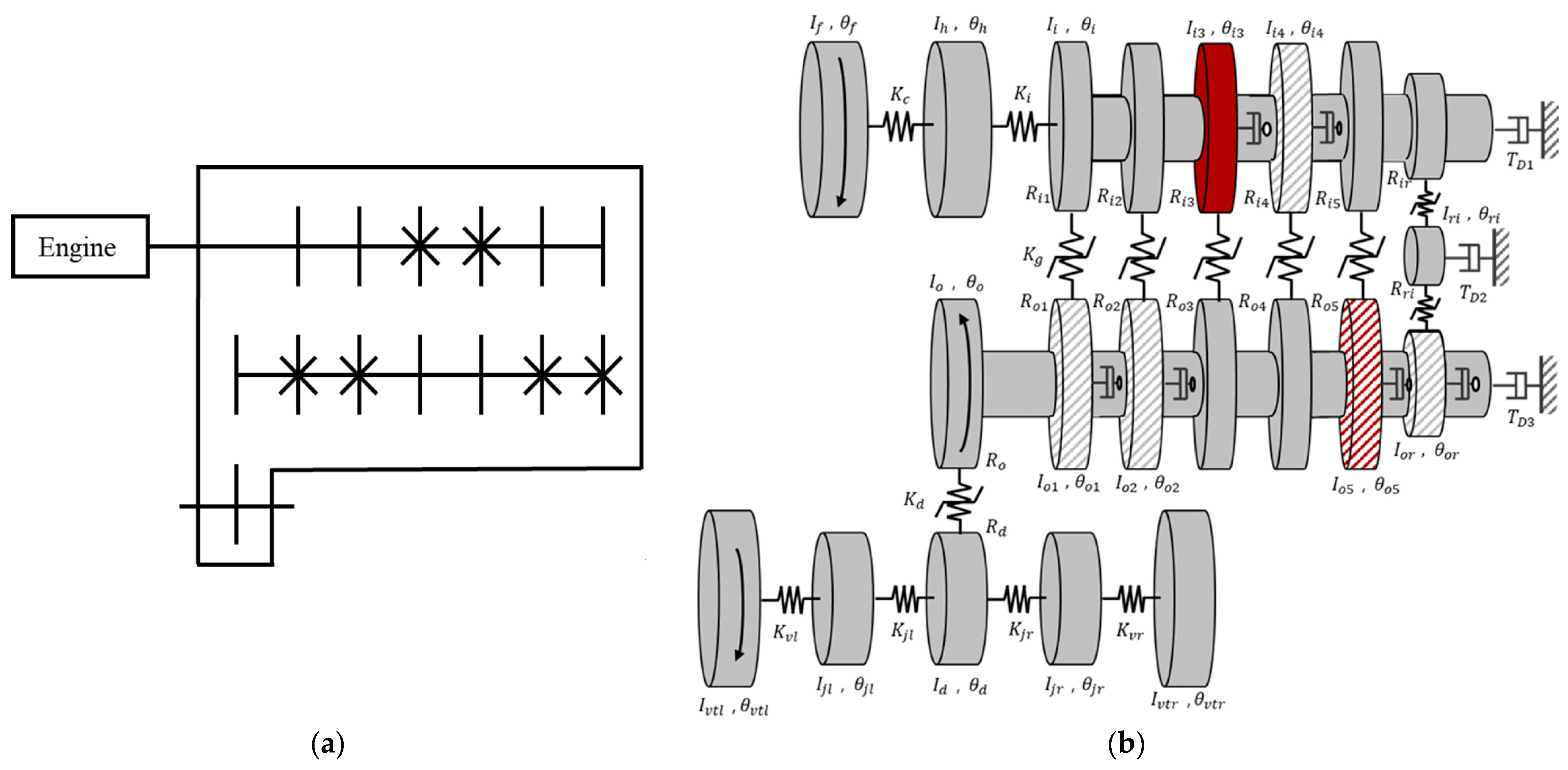
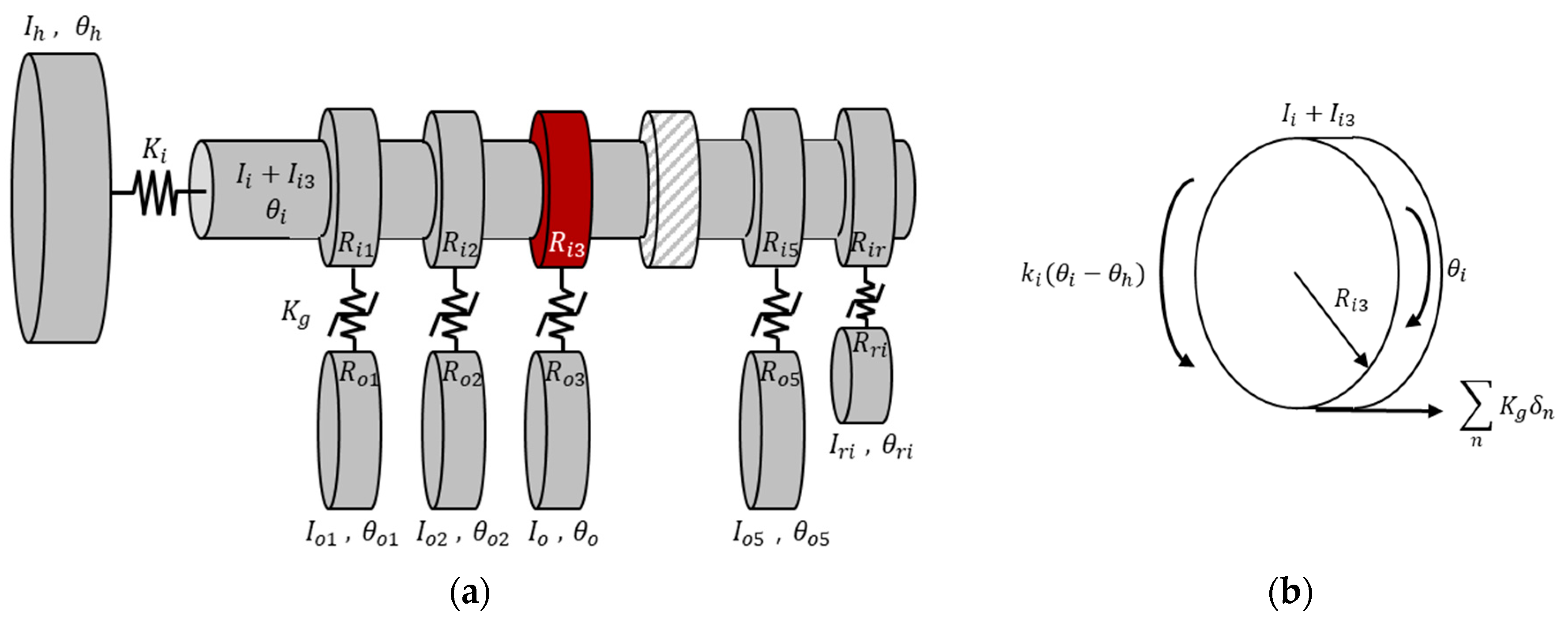
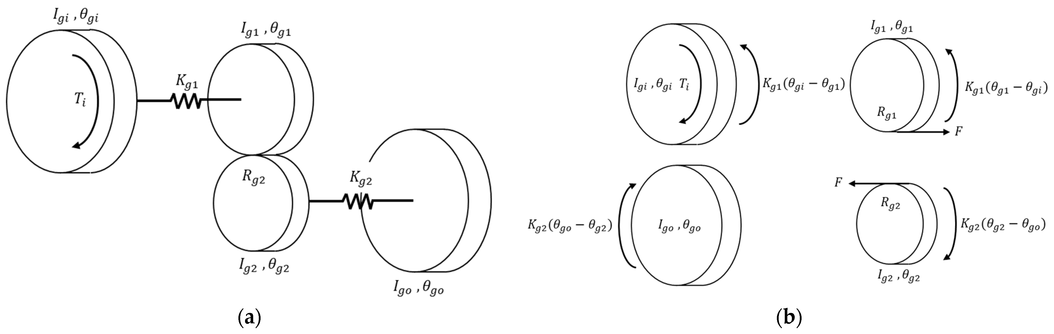
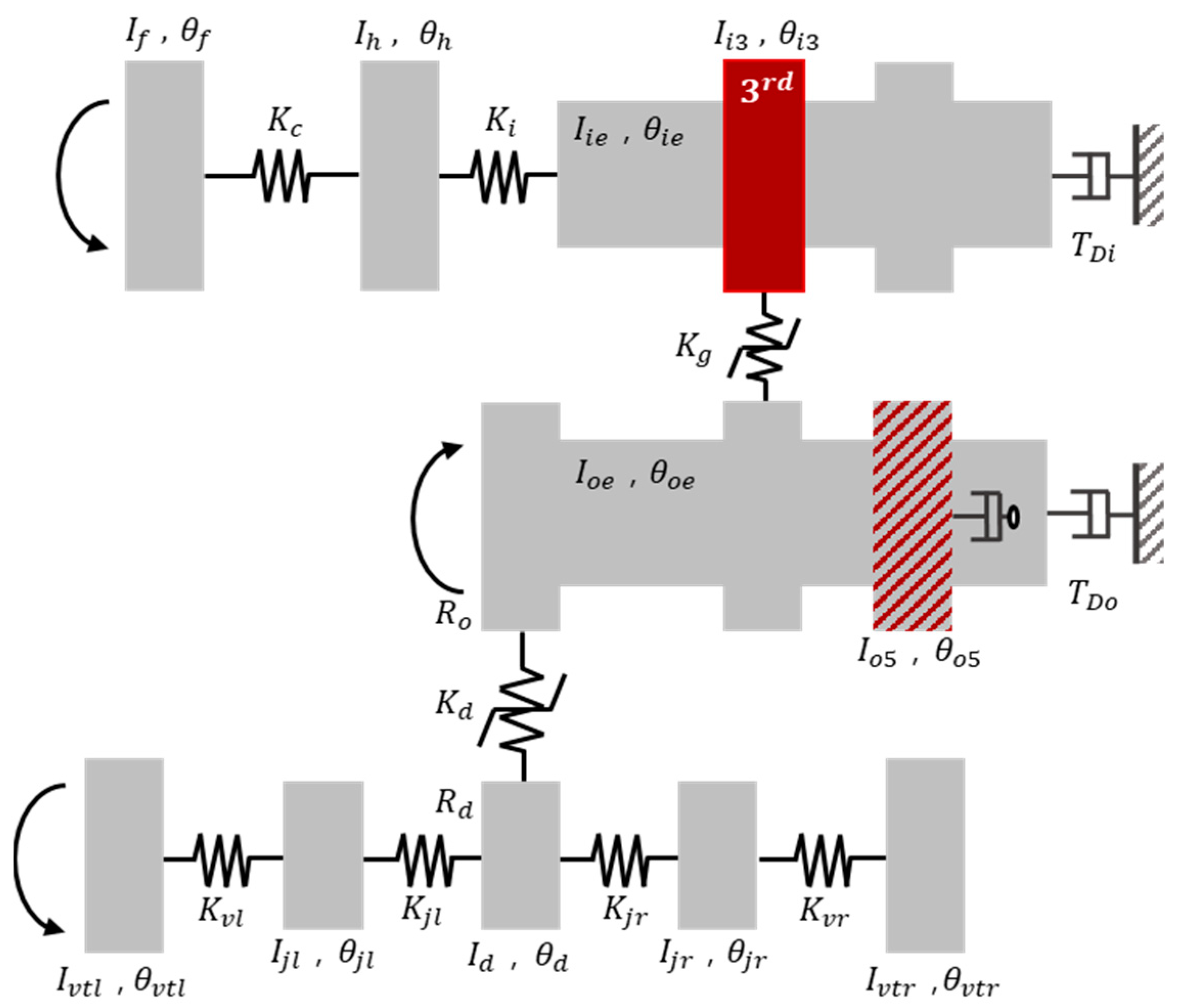
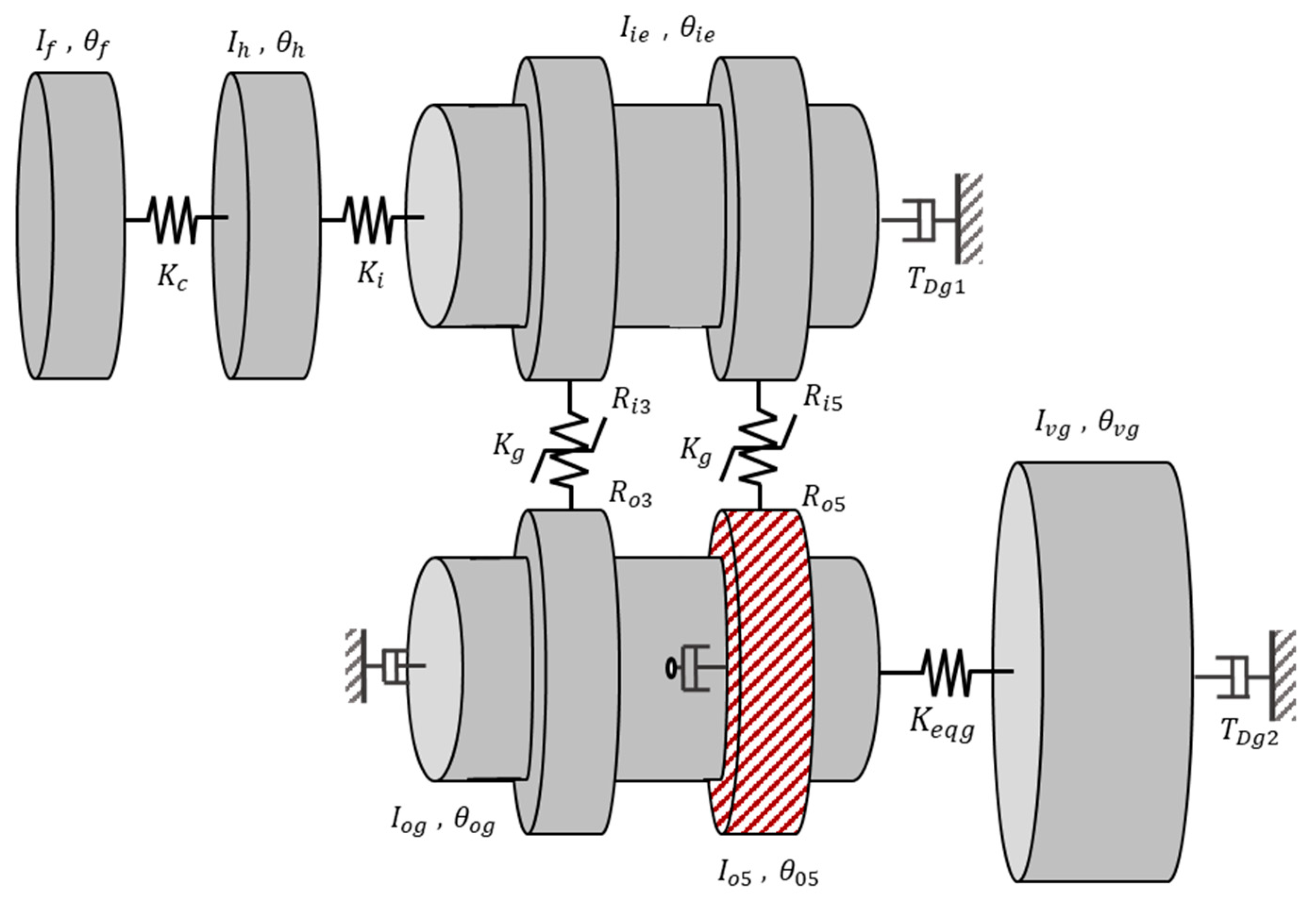
3.1. Modeling of the Torsional System
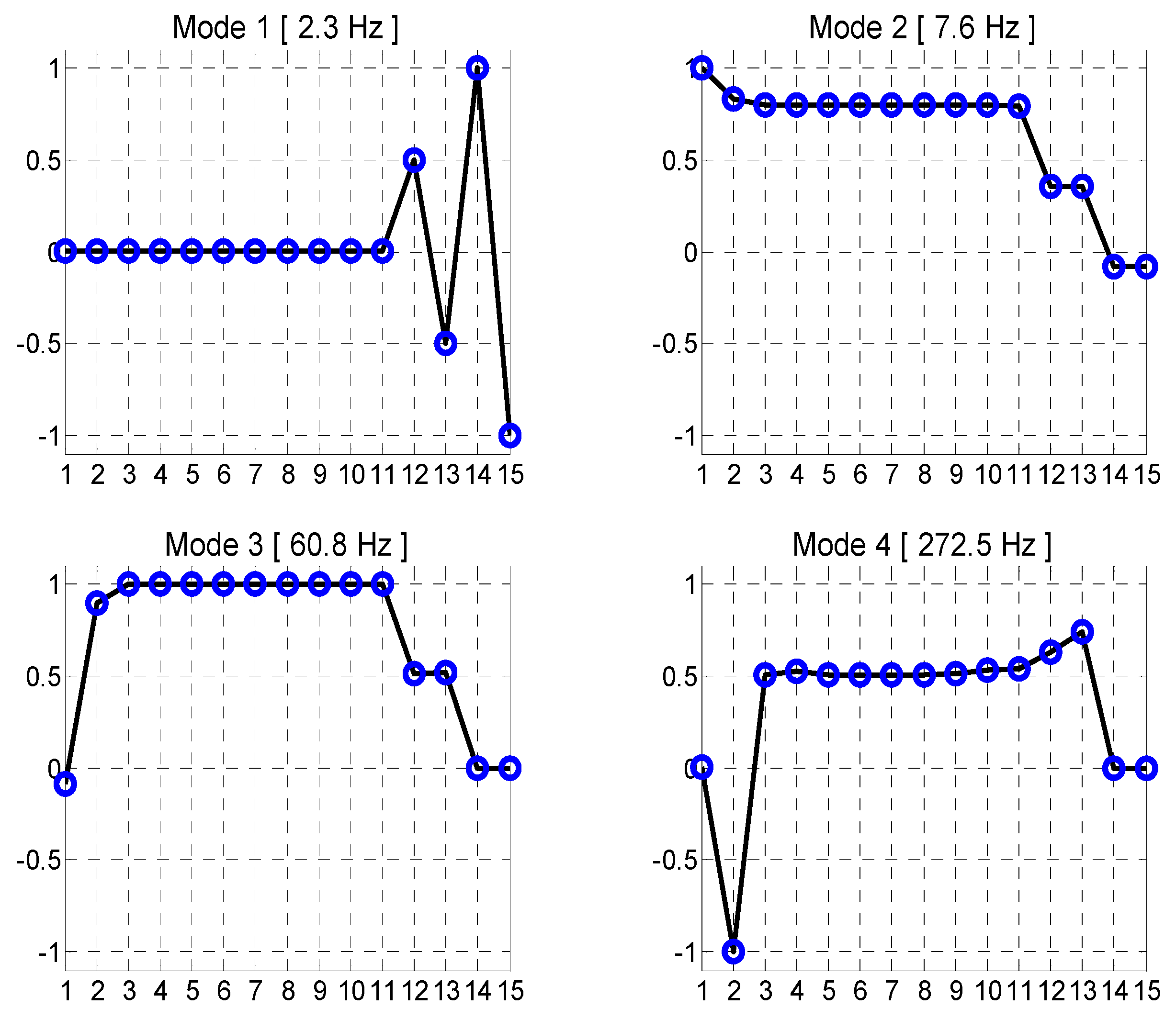
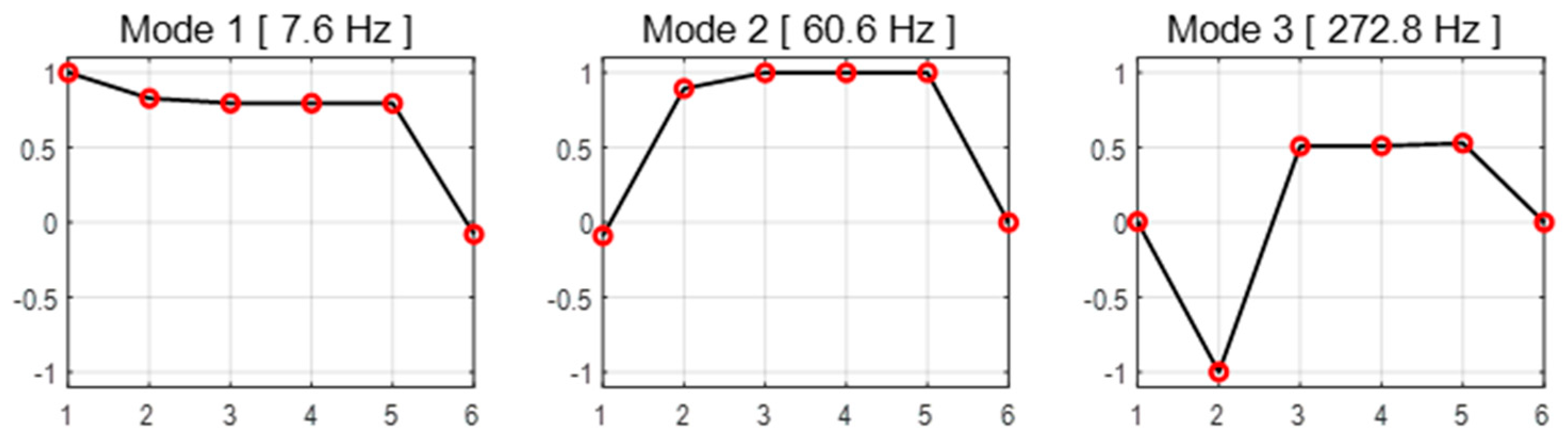
3.2. Modal Analysis of the Torsional System
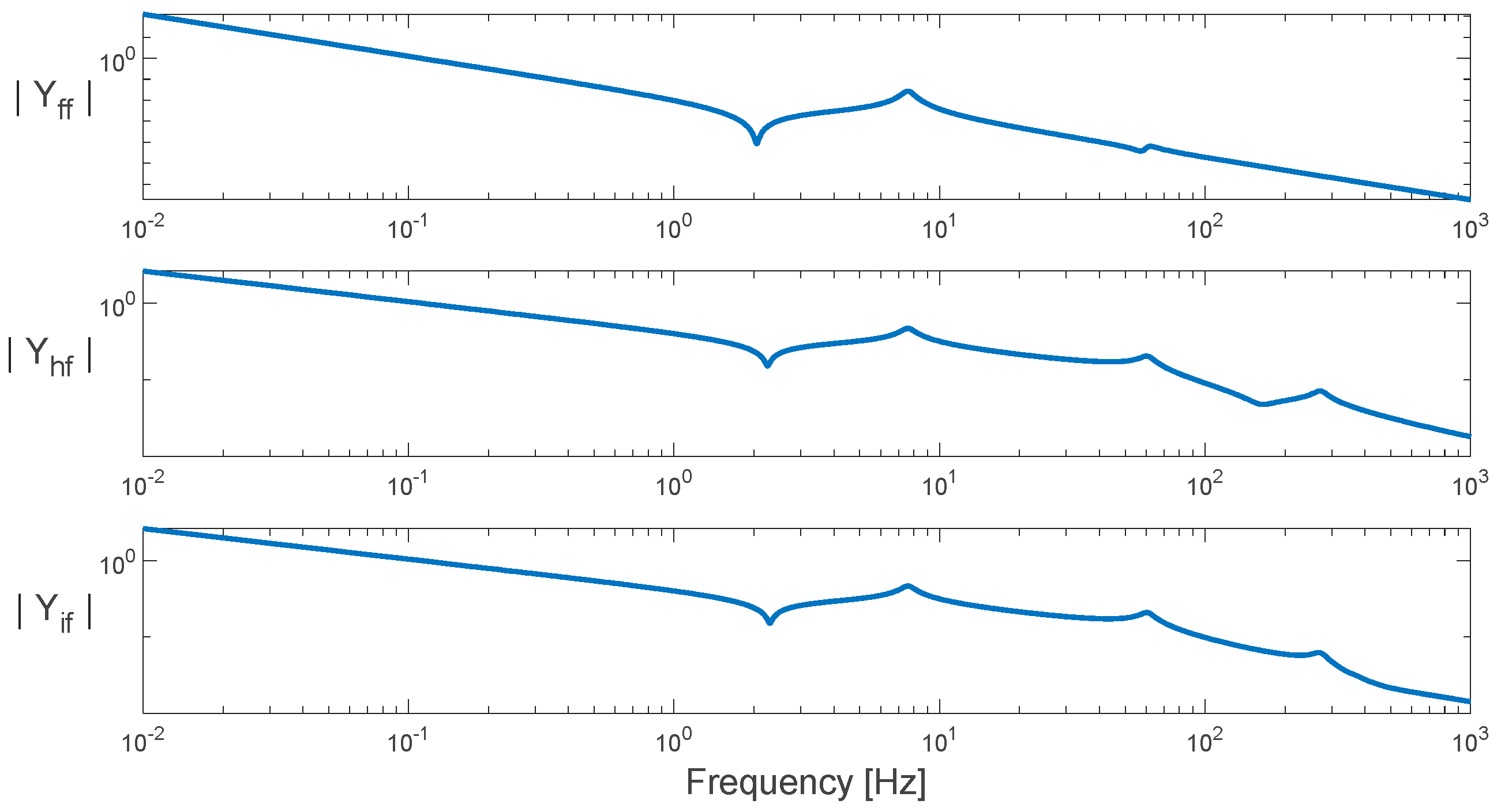
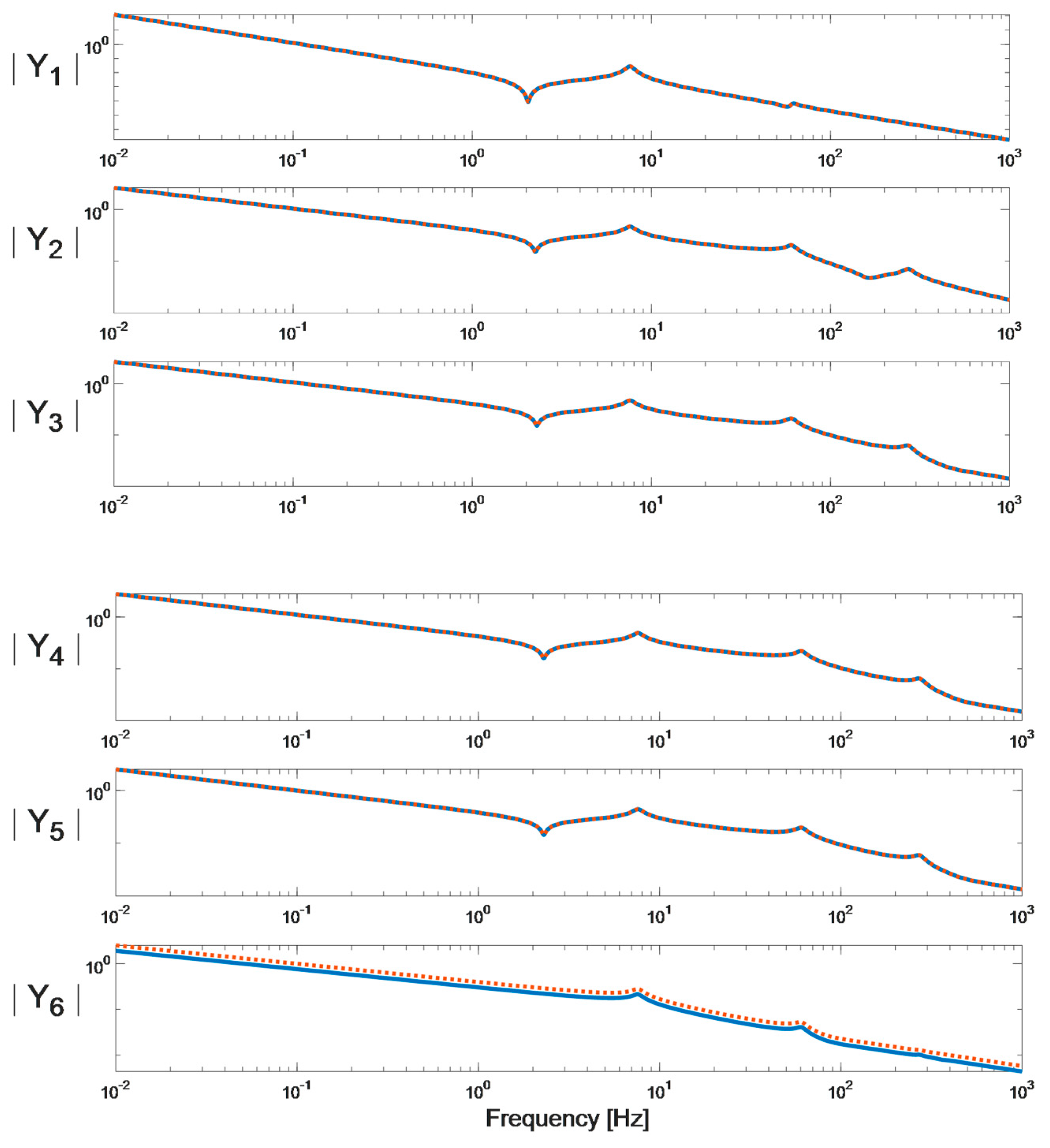
3.3. System Responses in the Frequency Domain
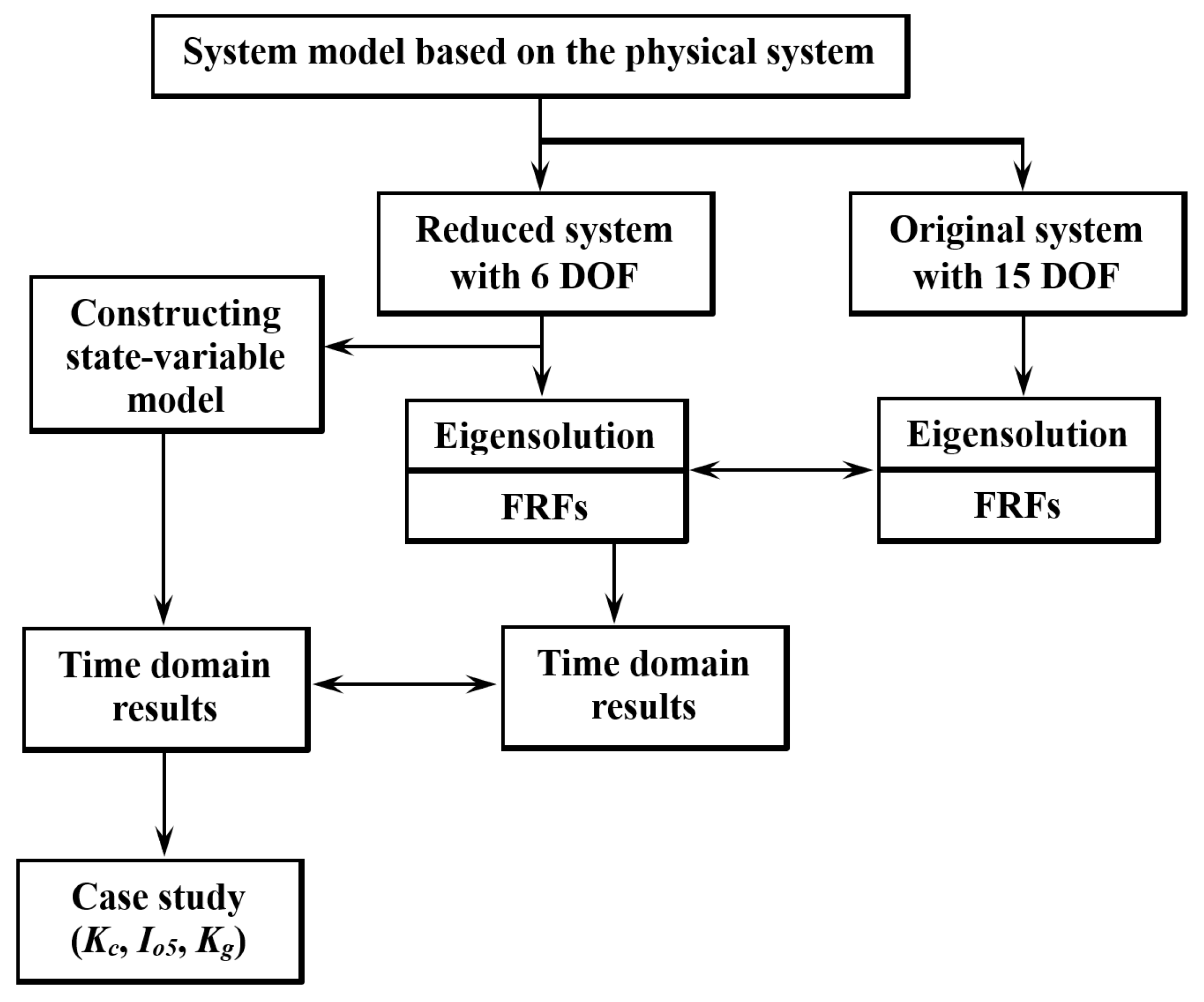
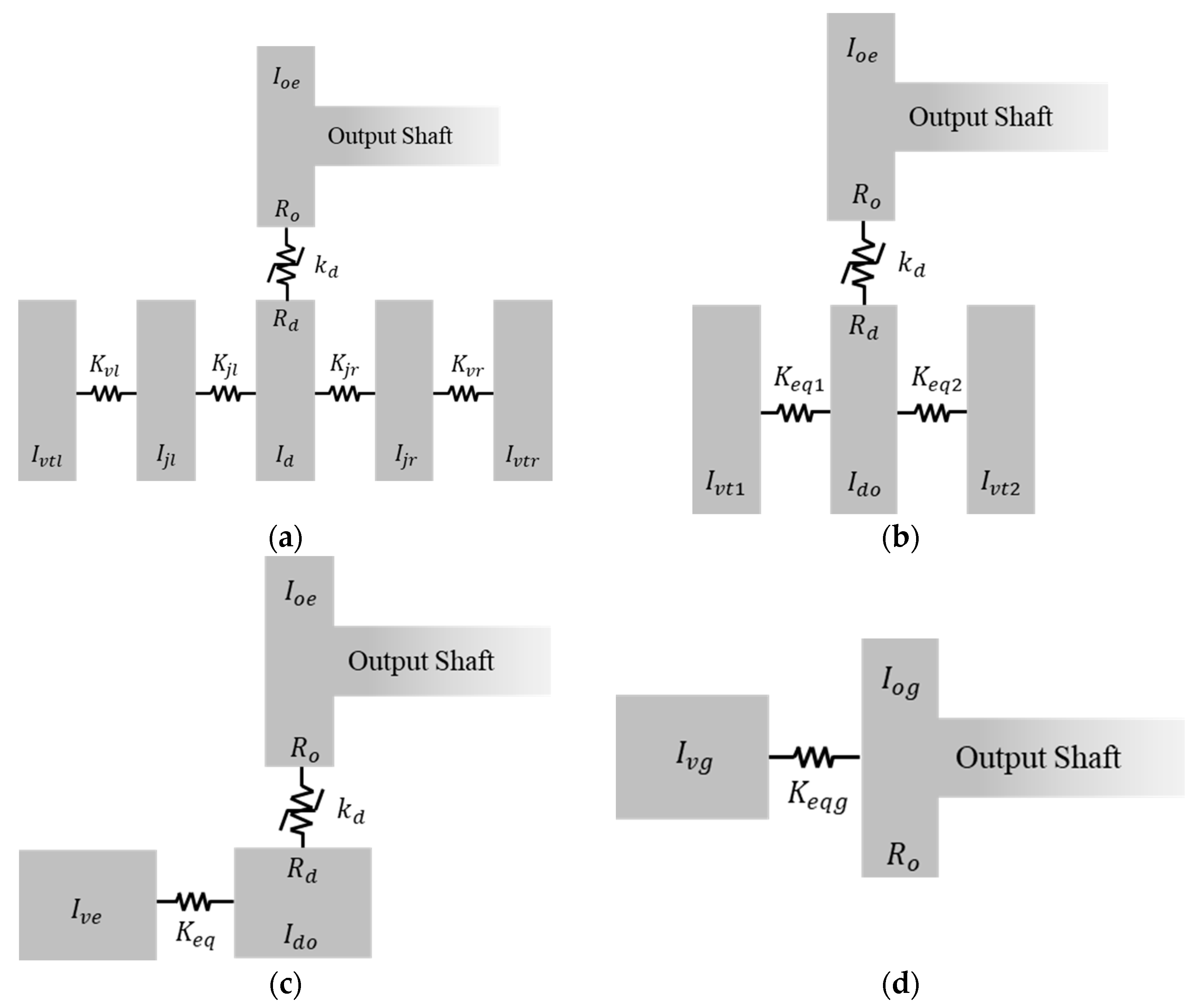
4. System Reduction and Validation with the Original System
5. Linear Analysis in the Time Domain
5.1. Time Responses Based on Modal Domain and FRFs
5.2. Time Responses Based on the State Variable Equation
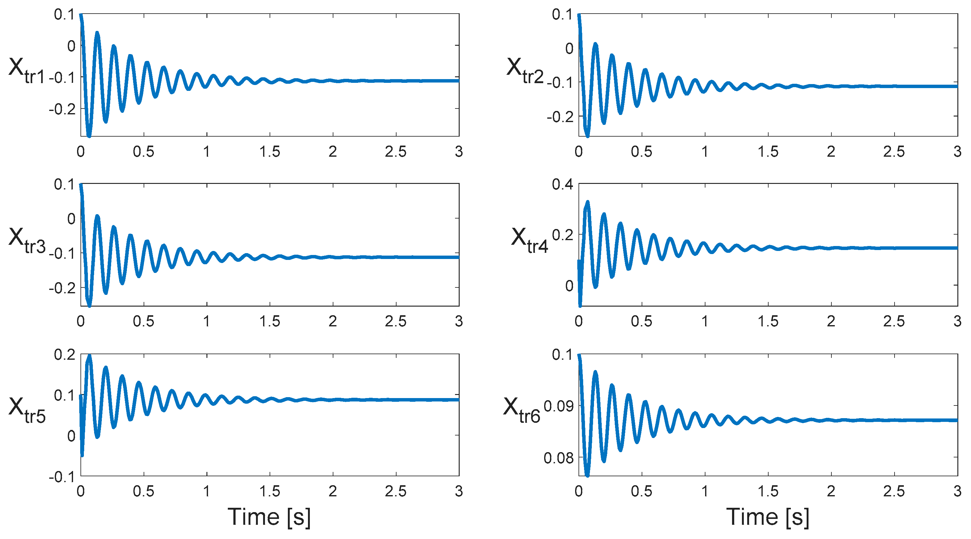
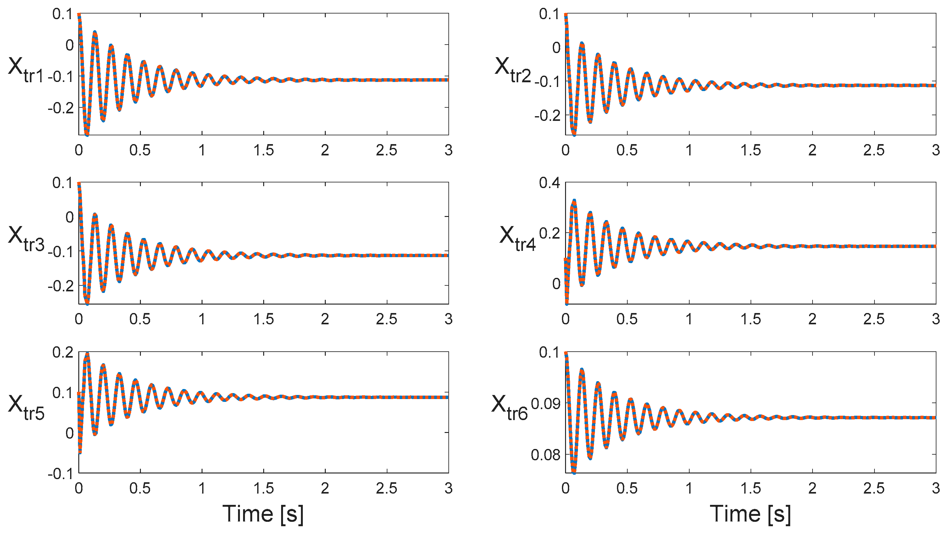
5.2.1. Transient Response
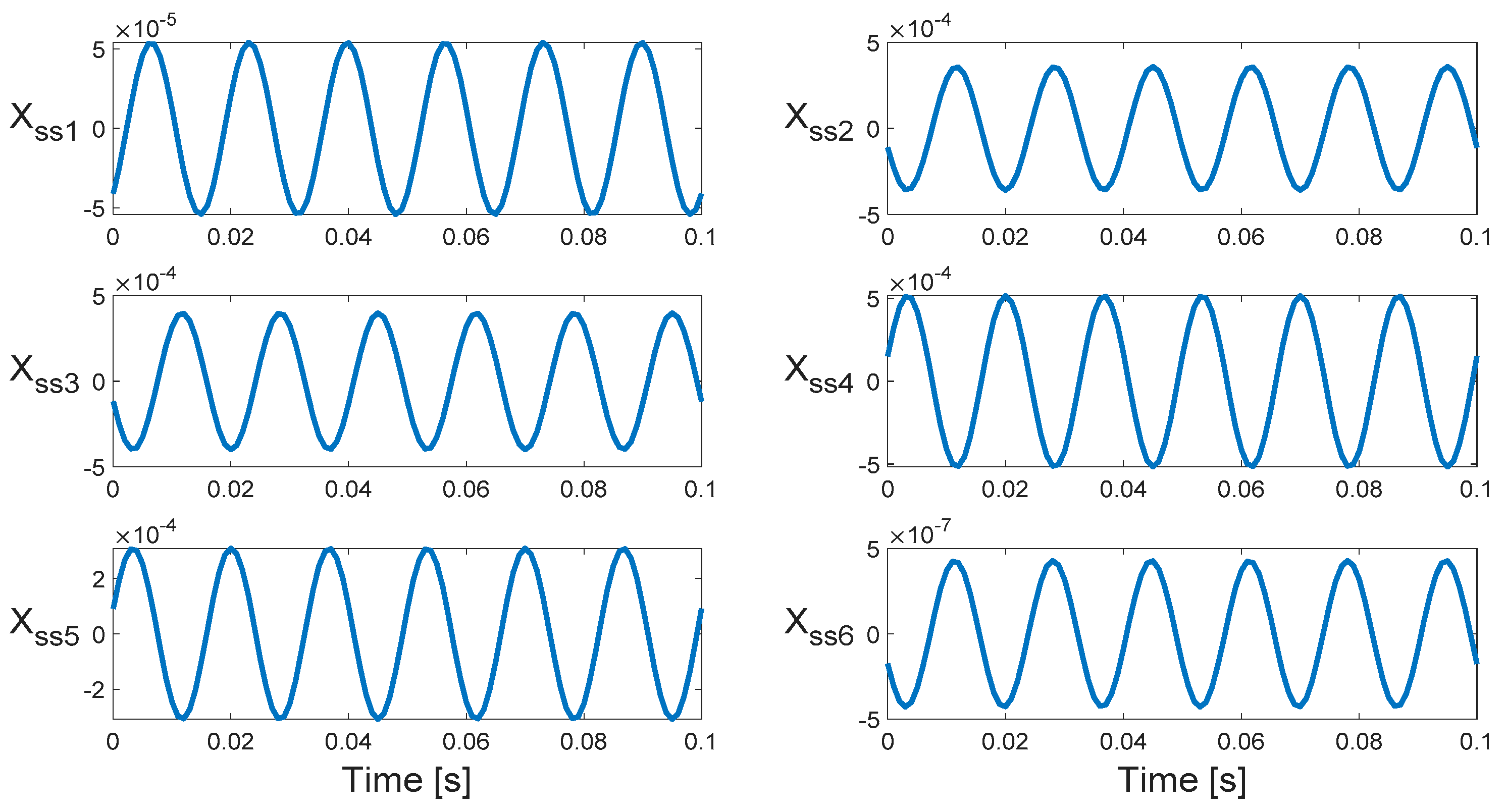
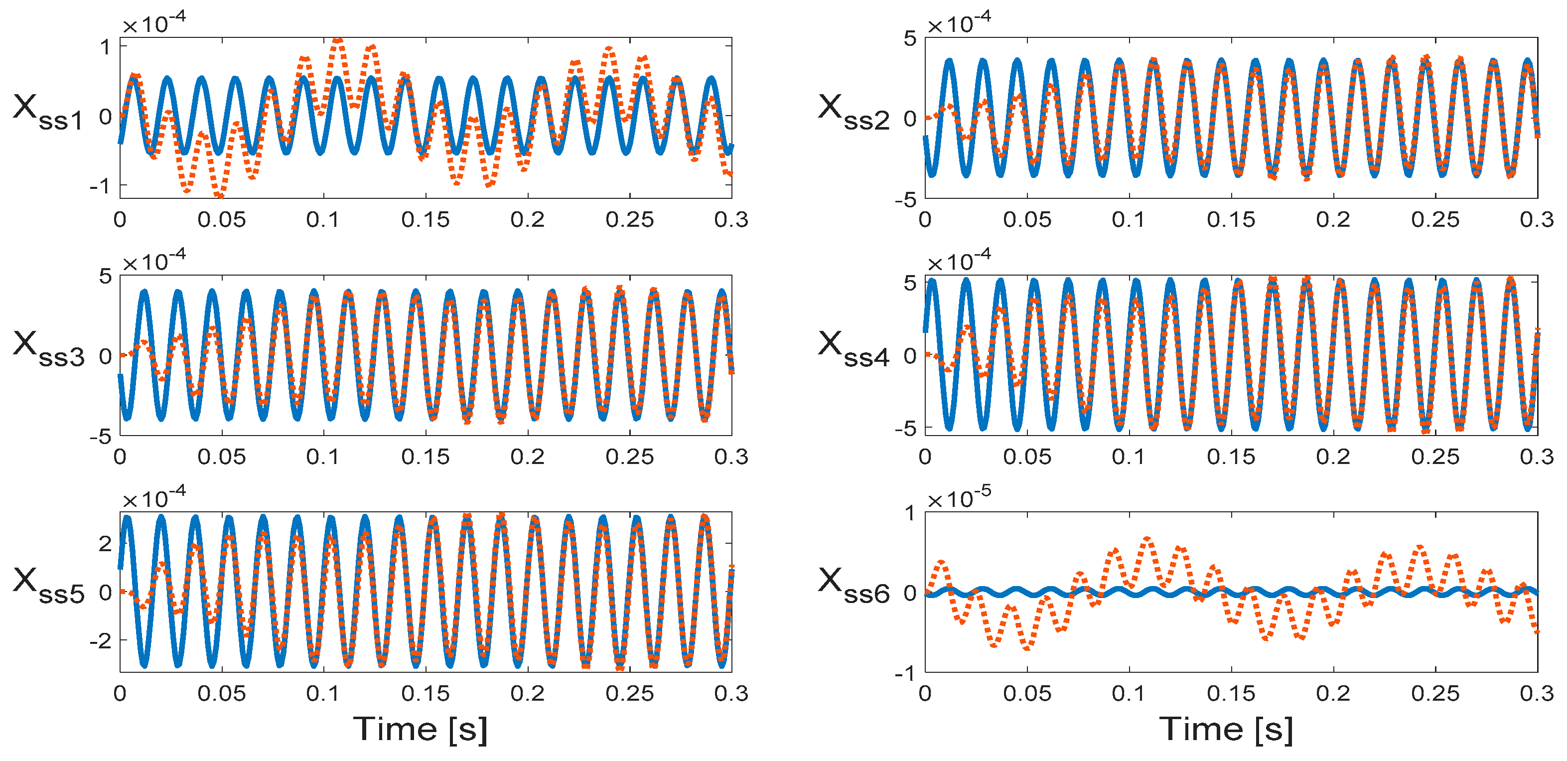
5.2.2. Steady-State Responses for Semi-Definite System
6. Case Study
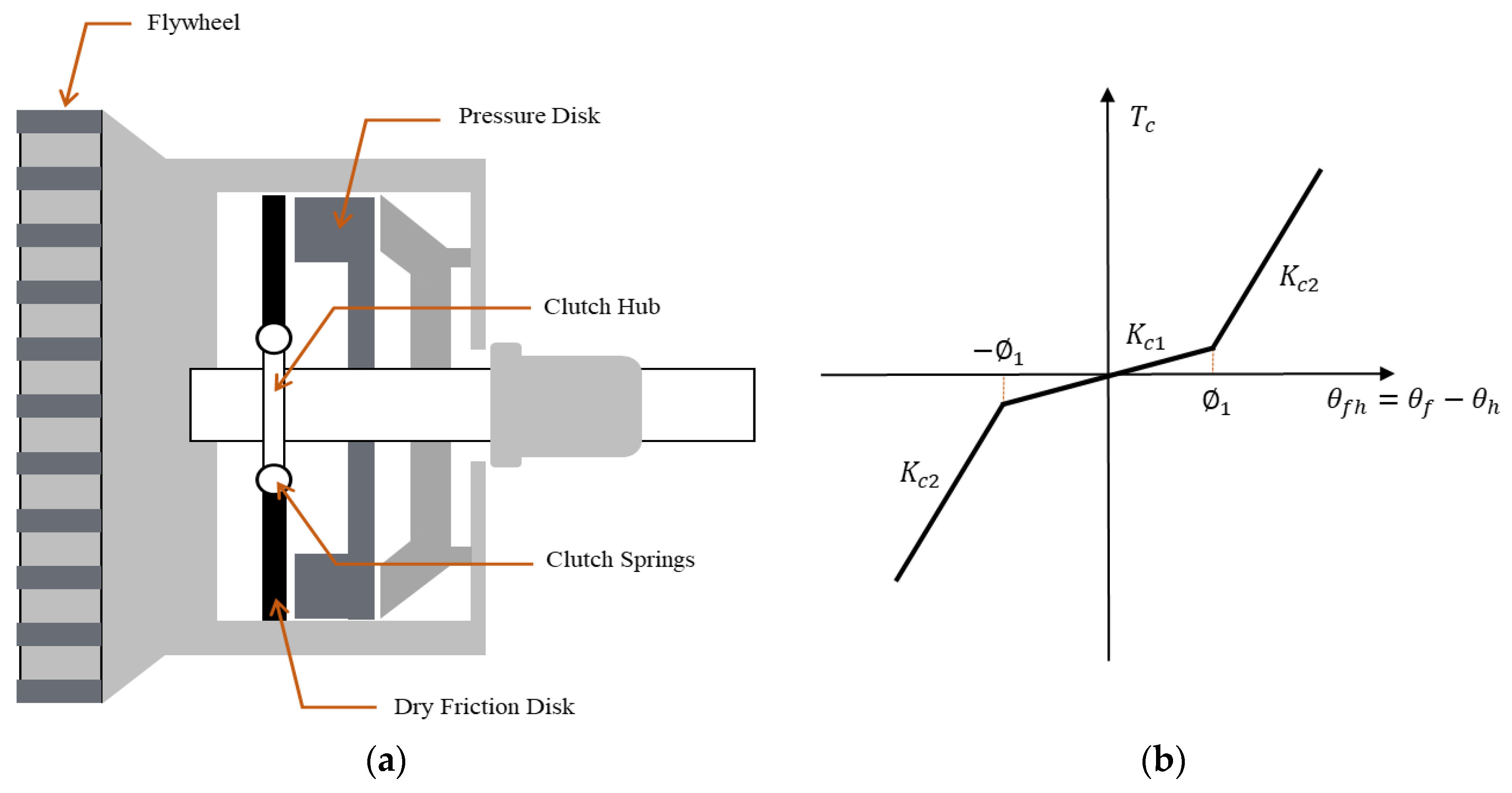
6.1. Case Study I: Clutch Stiffness Kc
6.2. Case Study II: Unloaded Gear Inertia Io5
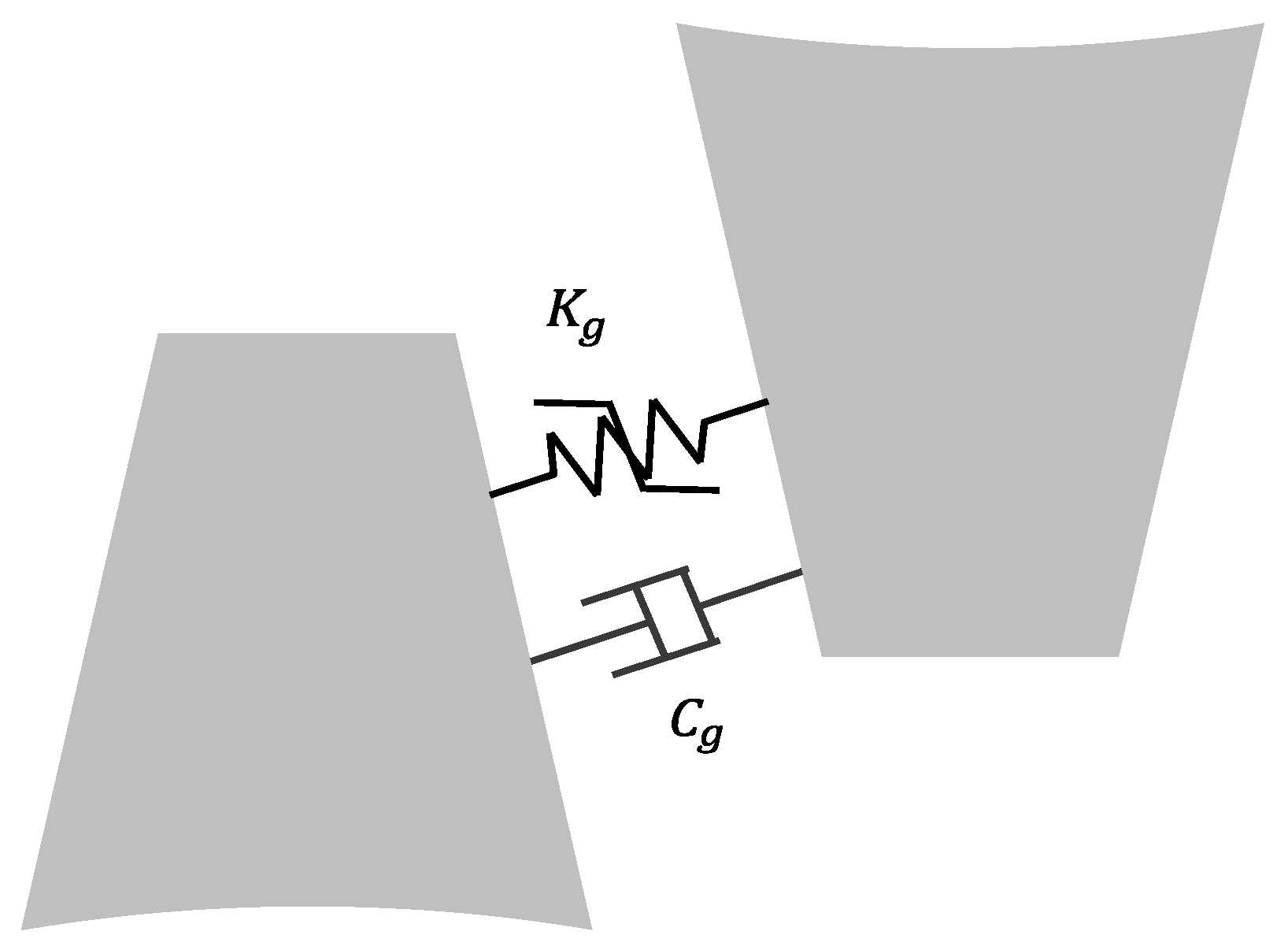
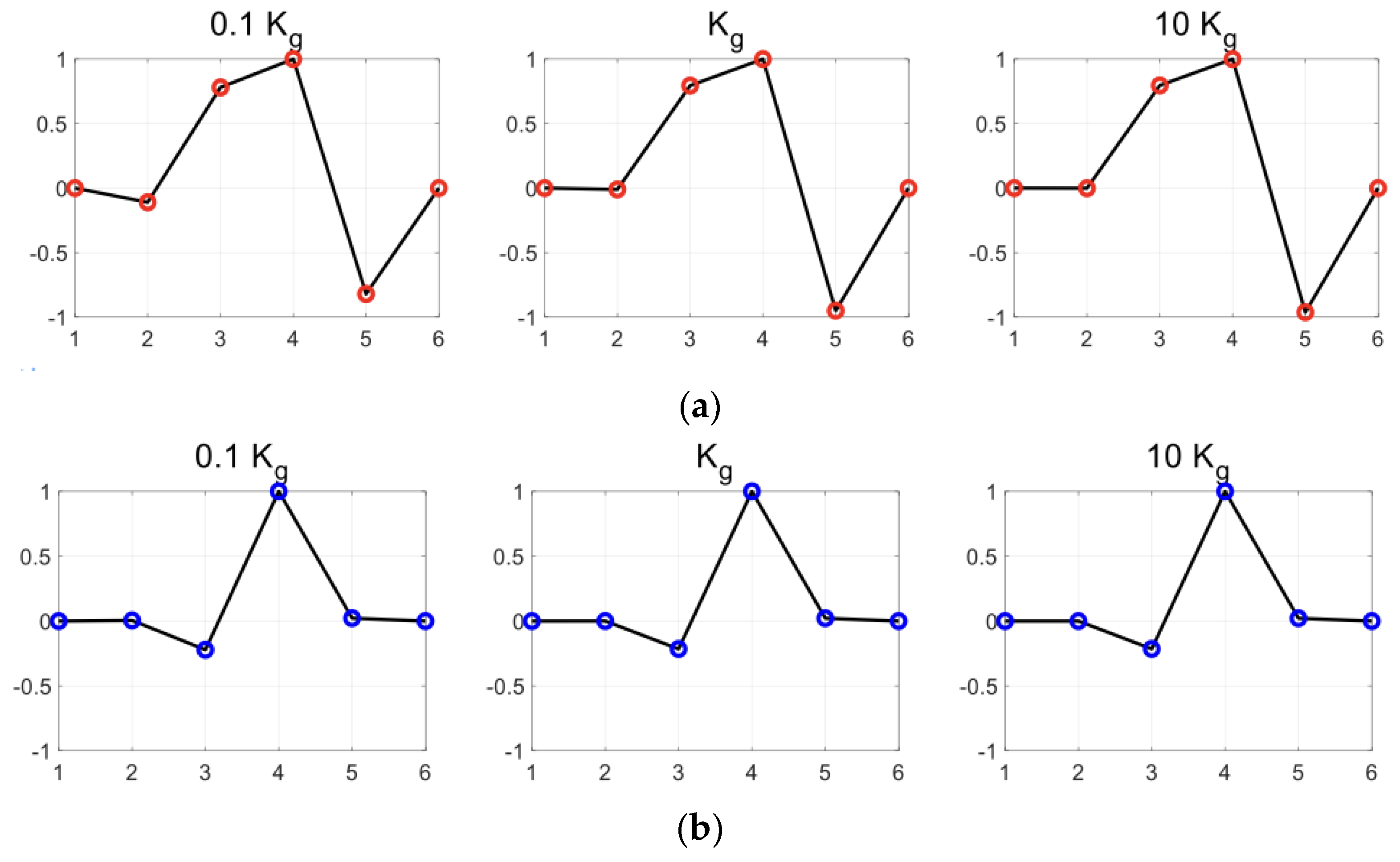
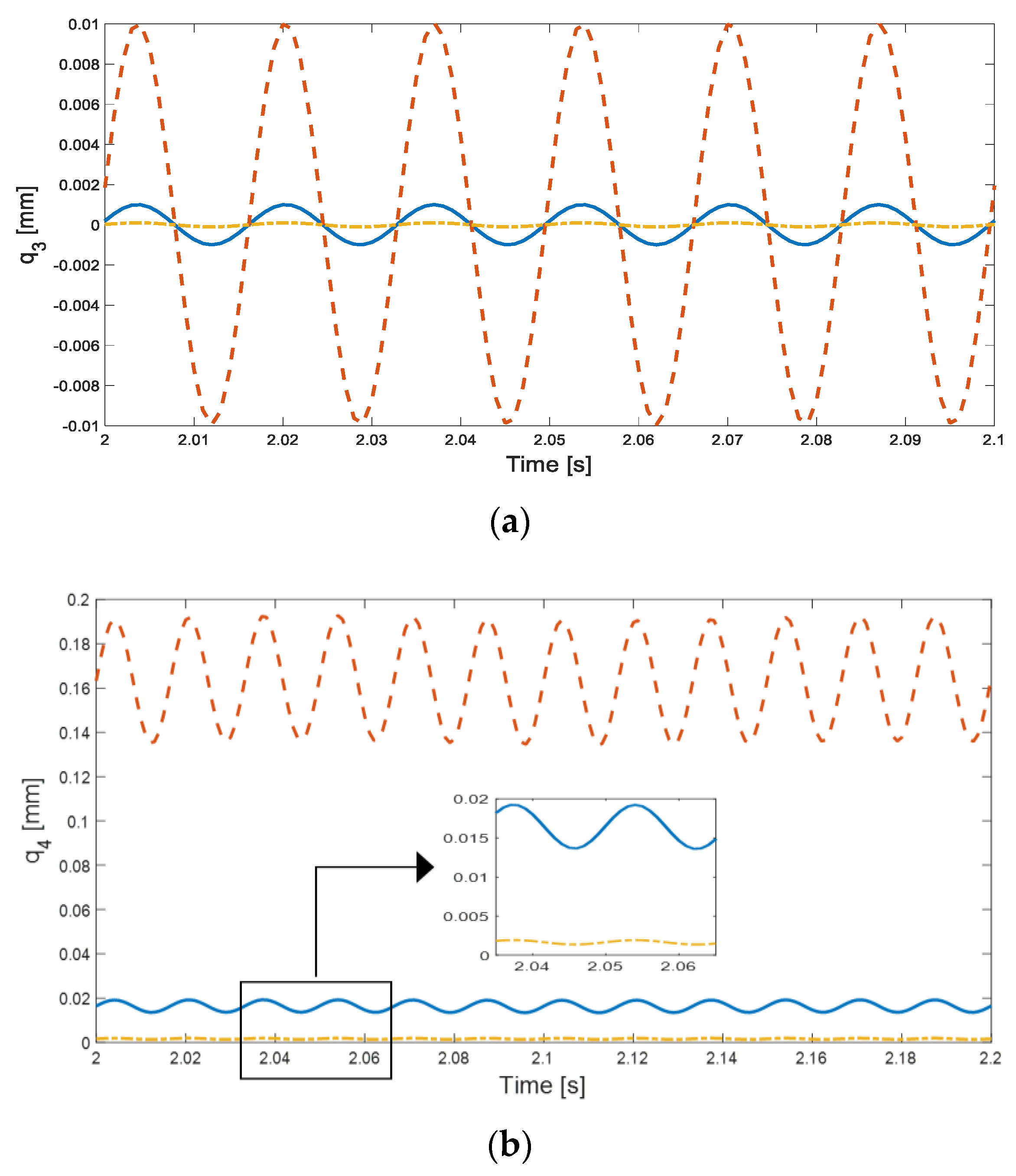
6.3. Case Study III: Gear Mesh Stiffness Kg
7. Conclusions
Author Contributions
Funding
Data Availability Statement
Conflicts of Interest
References
- Yoon, J.Y.; Singh, R. Effect of the multi-staged clutch damper characteristics on the transmission gear rattle under two engine conditions. Proc. Inst. Mech. Eng. Part D J. Automob. Eng. 2013, 227, 1273–1294. [Google Scholar] [CrossRef]
- Guo, D.; Zhou, Y.; Zhou, Y.; Wang, Y.; Chen, F.; Shi, X. Numerical and experimental study of gear rattle based on a refined dynamic model. Appl. Acoust. 2022, 185, 108407. [Google Scholar] [CrossRef]
- Zhou, Y.; Shi, X.; Guo, D.; Dazer, M.; Bertsche, B.; Mei, Z. Experimental investigation of gear rattle and nonlinear dynamic interaction in a dual-clutch transmission. Appl. Acoust. 2023, 204, 109233. [Google Scholar] [CrossRef]
- Diez-Ibarbia, A.; Fernandez-del-Rincon, P.; Garcia, P.; Viadero, F. Gear rattle dynamics under non-stationary conditions: The lubricant role. Mech. Mach. Theory 2020, 151, 103929. [Google Scholar] [CrossRef]
- Bozca, M. Transmission error model-based optimization of the geometric design parameters of an automotive transmission gearbox to reduce gear-rattle noise. Appl. Acoust. 2018, 130, 247–259. [Google Scholar] [CrossRef]
- Rigaud, E.; Liaudet, J.P. Investigation of gear rattle noise including visualization of vibro-impact regimes. J. Sound Vib. 2020, 467, 115026. [Google Scholar] [CrossRef]
- Donmez, A.; Kahraman, A. Influence of various manufacturing errors on gear rattle. Mech. Mach. Theory 2022, 173, 104868. [Google Scholar] [CrossRef]
- Singh, R.; Xie, H.; Comparin, R.J. Analysis of automotive neutral gear rattle. J. Sound Vib. 1989, 131, 177–196. [Google Scholar] [CrossRef]
- Pizzolante, F.; Battarra, M.; D’Elia, G.; Mucchi, E. A rattle index formulation for single and multiple branch geartrains. Mech. Mach. Theory 2021, 158, 104246. [Google Scholar] [CrossRef]
- Guo, D.; Ning, Q.; Ge, S.; Wang, Y.; Zhou, Y.; Zhou, Y.; Shi, X. Nonlinear characteristic analysis of gear rattle based on refined dynamic model. Nonlinear Dyn. 2022, 110, 3109–3133. [Google Scholar] [CrossRef]
- Shangguan, W.B.; Liu, X.L.; Yin, Y.; Rakheja, S. Modeling of automotive driveline system for reducing gear rattles. J. Sound Vib. 2018, 416, 136–153. [Google Scholar] [CrossRef]
- Trochon, E.P. Analytical Formulation of Automotive Drivetrain Rattle Problems. Master’s Thesis, The Ohio State University, Columbus, OH, USA, 1997. [Google Scholar]
- Idehara, S.J.; Flach, F.L.; Lemes, D. Modeling of nonlinear torsional vibration of the automotive powertrain. J. Vib. Control. 2018, 24, 1774–1786. [Google Scholar] [CrossRef]
- Beinstingel, A.; Parker, R.G.; Marburg, S. Experimental measurement and numerical computation of parametric instabilities in a planetary gearbox. J. Sound Vib. 2022, 536, 117160. [Google Scholar] [CrossRef]
- Pizzolante, F.; Battarra, M.; Mucchi, E. The role of gear layout and meshing phase for whine noise reduction in ordinary geartrains. Mech. Mach. Theory 2023, 181, 105209. [Google Scholar] [CrossRef]
- Palermo, A.; Britte, L.; Janssens, K.; Mundo, D.; Desmet, W. The measurement of Gear Transmission Error as an NVH indicator: Theoretical discussion and industrial application via low-cost digital encoders to an all-electric vehicle gearbox. Mech. Syst. Signal Process. 2018, 110, 368–389. [Google Scholar] [CrossRef]
- Mughal, H.; Sivayogan, G.; Nader, D.; Ramin, R. An efficient analytical approach to assess root cause of nonlinear electric vehicle gear whine. Nonlinear Dyn. 2022, 110, 3167–3186. [Google Scholar] [CrossRef]
- Yoo, H.G.; Chung, W.J.; Kim, B.S.; Park, Y.J.; Kang, M.R.; Lee, H.K.; Kim, M.S.; Lee, K.S. Effect of hybrid metal-composite gear on the reduction of dynamic transmission error. J. Mech. Sci. 2023, 37, 3445–3457. [Google Scholar] [CrossRef]
- Barthod, M.; Hayne, B.; Tébec, J.L.; Pin, J.C. Experimental study of gear rattle excited by a multi-harmonic excitation. Appl. Acoust. 2007, 68, 1003–1025. [Google Scholar] [CrossRef]
- Cui, L.; Liu, T.; Huang, J.; Wang, H. Improvement on meshing stiffness algorithms of gear with peeling. Symmetry 2019, 11, 609. [Google Scholar] [CrossRef]
- Chen, L.; Zhang, X.; Yan, Z.; Zeng, R. Matching model of dual mess flywheel and power transmission based on the structural sensitivity analysis method. Symmetry 2019, 11, 187. [Google Scholar] [CrossRef]
- Ren, Z.; Xin, X.; Sun, G.; Wei, X. The effect of gear meshing on the high-speed vehicle dynamics. Veh. Syst. Dyn. 2021, 59, 743–764. [Google Scholar] [CrossRef]
- Garvey, S.D.; Penny, J.E.T.; Friswell, M.I. The relationship between the real and imaginary parts of complex modes. J. Sound Vib. 1998, 212, 75–83. [Google Scholar] [CrossRef]
- Rubens, G.S.J. Advanced in the Theory of Linear Dynamical Systems through Coordinate Decoupling. Ph.D. Thesis, University of California, Berkeley, CA, USA, 2019. [Google Scholar]
- Tisseur, F.; Meerbergen, K. The quadratic eigenvalue problem. SIAM Rev. 2006, 43, 235–286. [Google Scholar] [CrossRef]
- Afolabi, D. Linearization of the quadratic eigenvalue problem. Comput. Struct. 1987, 26, 1039–1040. [Google Scholar] [CrossRef]
- Chen, H.C.; Taylor, R.L. Solution of eigenproblems for damped structural systems by the Lanczos algorithm. Comput. Struct. 1988, 30, 151–161. [Google Scholar] [CrossRef]
- Datta, B.N.; Elhay, S.; Ram, Y.M. Orthogonality and partial pole assignment for the symmetric definite quadratic pencil. Linear Algebra Appl. 1997, 257, 29–48. [Google Scholar] [CrossRef]
- Golub, G.H. Some modified matrix eigenvalue problems. SIAM Rev. 1973, 15, 318–334. [Google Scholar] [CrossRef]
- Arnoldi, W.E. The principle of minimized iterations in the solution of the matrix eigenvalue problem. Q. Appl. Math. 1951, 9, 17–29. [Google Scholar] [CrossRef]
- Den Hartog, J.P. Mechanical Vibrations; Dover Publications: New York, NY, USA, 1985. [Google Scholar]
- Inman, D.J. Engineering Vibration; Pearson Education Asia: Seoul, Korea, 2013. [Google Scholar]
- Luis, J.; Zabala, M.; All, M.; Connor, J.J.; Sussman, J.M. State-Space Formulation for Structural Dynamics. Master’s Thesis, Massachusetts Institute of Technology, Cambridge, MA, USA, 1996. [Google Scholar]
- Koch, U.; Wiedemann, D.; Sundqvist, N.; Ulbrich, H. State-space modelling and decoupling control of electromagnetic actuators for car vibration excitation. In Proceedings of the IEEE 2009 International Conference on Mechatronics, ICM 2009, Málaga, Spain, 14–17 April 2009. [Google Scholar]
- Leonard, I.E. The matrix exponential. SIAM Rev. 1996, 38, 507–512. [Google Scholar] [CrossRef]
- Bay, J. Fundamentals of Linear State Space Systems; WCB McGraw-Hill: Boston, MA, USA, 1999. [Google Scholar]
- Macías, J.A.R.; Expósito, A.G.; Soler, A.B. A comparison of techniques for state-space transient analysis of transmission lines. IEEE Trans. Power Deliv. 2005, 20, 894–903. [Google Scholar] [CrossRef]
- Rook, T.E.; Singh, R. Modeling of automotive gear rattle phenomenon: State of the art. J. Passeng. Cars 1995, 104, 2332–2343. [Google Scholar]
- Padmanabhan, C.; Barlow, R.C.; Rook, R.C.; Singh, R. Computational issues associated with gear rattle analysis. J. Mech. Des. 1995, 117, 185–192. [Google Scholar] [CrossRef]
- Curtis, S.; Pears, J.; Palmer, D.; Eccles, M.; Poon, A.; Kim, M.G.; Jeon, G.Y.; Kim, J.K.; Joo, S.H. An analytical method to reduce gear whine noise, including validation with test data. J. Passeng. Car Mech. Syst. J. 2005, 114, 2195–2202. [Google Scholar]


 , 15-DOF;
  , 6-DOF.


 , using the modal analysis;
  , using the state variable equation.
, using the modal analysis; , using the state variable equation.
, using the state variable equation.
, using the modal analysis; , using the state variable equation.
 , using the FRFs;
  , using the state variable equation.
, using the FRFs; , using the state variable equation.
, using the state variable equation.
, using the FRFs; , using the state variable equation.
 , using the FRFs;
  , using the state variable equation.
, using the FRFs; , using the state variable equation.
, using the state variable equation.
, using the FRFs; , using the state variable equation.


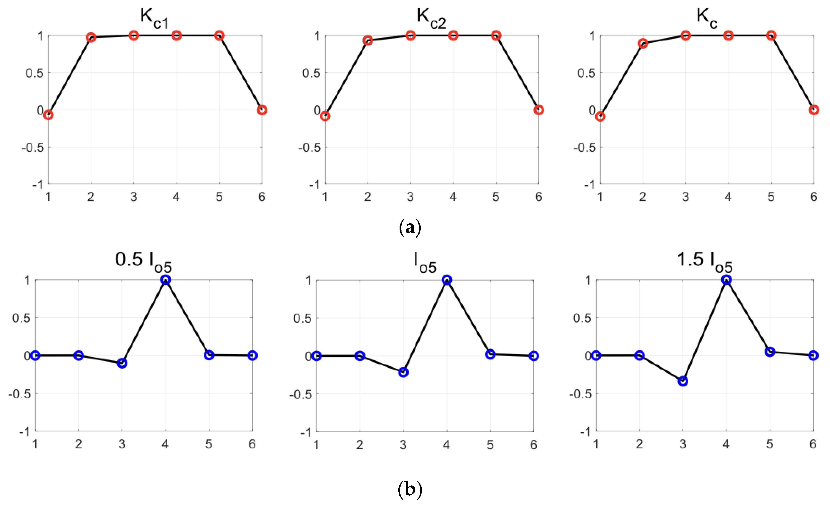
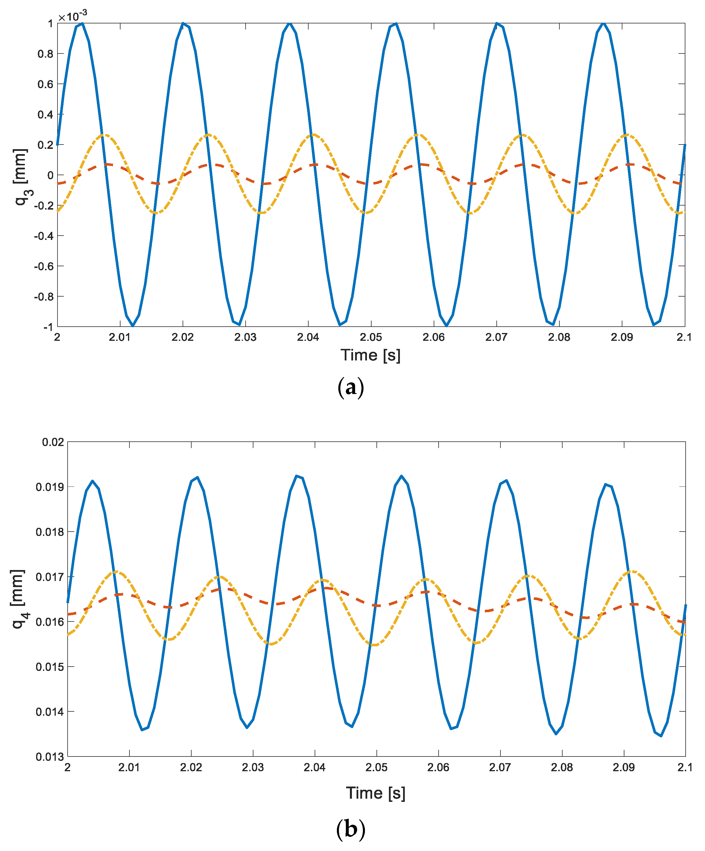
 , Kc1;
  , Kc;
, Kc;  , Kc2.
, Kc1; , Kc; , Kc2.
, Kc2.
, Kc1; , Kc; , Kc2.
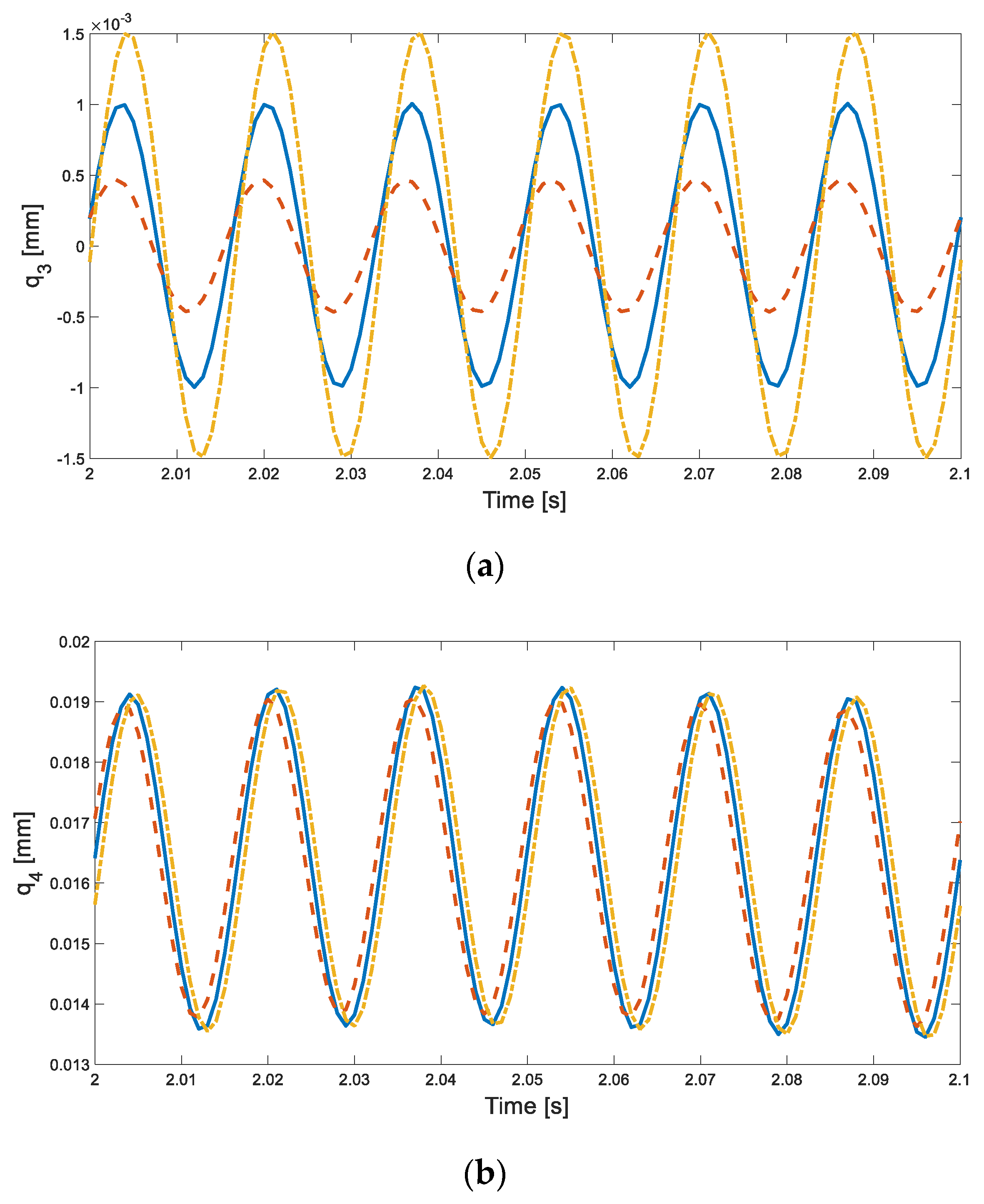
 , 0.5 Io5;
  ,1 Io5;
  , 1.5 Io5.
, 0.5 Io5; ,1 Io5; , 1.5 Io5.
, 1.5 Io5.
, 0.5 Io5; ,1 Io5; , 1.5 Io5.

 , 0.1 Kg;
  ,1 Kg;
  , 10 Kg.
, 0.1 Kg; ,1 Kg; , 10 Kg.
, 10 Kg.
, 0.1 Kg; ,1 Kg; , 10 Kg.

| Inertia (Description) | Values (kg∙m2) | Inertia | Values (kg∙m2) |
|---|---|---|---|
| If (Flywheel) | 1.38 × 10⁻¹ | Io5 (5th gear on output shaft) | 5.23 × 10⁻⁴ |
| Ih (Clutch hub) | 5.76 × 10⁻³ | Iri (Idler) | 4.35 × 10⁻⁴ |
| Ii (Input shaft) | 3.10 × 10⁻³ | Ior (Reverse gear on output shaft) | 1.33 × 10⁻³ |
| Io (Output shaft) | 25.33 × 10⁻³ | Id (Differential) | 2.15 × 10⁻² |
| Ii3 (3rd gear on input shaft) | 5.80 × 10⁻⁴ | Ijl (Left cv joint) | 3.91 × 10⁻³ |
| Ii4 (4th gear on input shaft) | 8.73 × 10⁻⁴ | Ijr (Right cv joint) | 4.35 × 10⁻³ |
| Io1 (1st gear on output shaft) | 2.60 × 10⁻³ | Ivtl (Left tire and vehicle) | 23.9591 |
| Io2 (2nd gear on output shaft) | 1.39 × 10⁻³ | Ivtr (Right tire and vehicle) | 23.9591 |
| Stiffness (Description) | Values (N∙m∙rad−1) | Stiffness | Values (N∙m−1) |
|---|---|---|---|
| Ki (Input shaft stiffness) | 10,000 | Kg (Gear mesh stiffness) | 2.7 × 10⁸ |
| Kjl, Kjr (Stiffness between left or right drive shaft and differential) | 10,000 | Kd (Gear mesh stiffness between output shaft and differential) | 2.7 × 10⁸ |
| Kvl, Kvr (Stiffness between left or right cv joint and vehicle) | 10,000 | ||
| Kc (Clutch stiffness) | 1838 |
| Radius (Description) | Values (mm) | Radius | Values (mm) |
|---|---|---|---|
| Ri1 (1st gear on input shaft) | 18.30 | Ro2 (2nd gear on output shaft) | 51.99 |
| Ri2 (2nd gear on input shaft) | 29.51 | Ro3 (3rd gear on output shaft) | 46.01 |
| Ri3 (3rd gear on input shaft) | 35.50 | Ro4 (4th gear on output shaft) | 39.55 |
| Ri4 (4th gear on input shaft) | 41.95 | Ro5 (5th gear on output shaft) | 35.58 |
| Ri5 (5th gear on input shaft) | 45.92 | Ror (Reverse gear on output shaft) | 54.95 |
| Rir (Reverse gear on input shaft) | 16.36 | Ro (Final gear on output shaft) | 26.63 |
| Rri (Idler) | 40.14 | Rd (Final gear on differential) | 103.37 |
| Ro1 (1st gear on output shaft) | 63.20 |
| Mode | Description | Natural Frequency (Hz) |
|---|---|---|
| 1 | Hopping mode (f1) | 2.3 |
| 2 | Driveline surging mode (f2) | 7.6 |
| 3 | Clutch spring mode (f3) | 60.8 |
| 4 | Clutch + input shaft mode (f4) | 272.5 |
| Natural Frequency (Hz) | 6-DOF | 15-DOF |
|---|---|---|
| f1 | 7.6 | 2.3 |
| f2 | 60.6 | 7.6 |
| f3 | 272.8 | 60.8 |
| f4 | 1846.3 | 272.5 |
| Natural Frequency (Hz) | Kc1 | Kc2 | Original Kc |
|---|---|---|---|
| (595.8 N∙m∙rad−1) | (1216.9 N∙m∙rad−1) | (1838 N∙m∙rad−1) | |
| f1 | 6.6 | 7.3 | 7.6 |
| f2 | 40.6 | 51.8 | 60.6 |
| f3 | 266.0 | 269.4 | 272.8 |
| f4 | 1845.7 | 1845.7 | 1846.3 |
| f5 | 4484.9 | 4484.9 | 4485.7 |
| 2nd Mode Shape | Kc1 | Kc2 | Kc |
|---|---|---|---|
| 1. flywheel | −0.0693 | −0.0847 | −0.0903 |
| 2. clutch hub | 0.9742 | 0.9328 | 0.8930 |
| 3. input shaft | 0.9999 | 0.9997 | 0.9992 |
| 4. unloaded gear | 1 | 0.9999 | 0.9994 |
| 5. output shaft | 0.9996 | 1 | 1 |
| 6. vehicle + wheel | −0.0032 | −0.0020 | −0.0014 |
| Peak-to-Peak Value q3 (mm) | Peak-to-Peak Value q4 (mm) | |
|---|---|---|
| Kc1 (595.8 N∙m∙rad−1) | 1.2723 × 10⁻⁴ | 3.9210 × 10⁻⁴ |
| Kc2 (1216.9 N∙m∙rad−1) | 5.1967 × 10⁻⁴ | 15 × 10−4 |
| Original Kc (1838 N∙m∙rad−1) | 20 × 10−4 | 56 × 10−4 |
| Natural Frequency (Hz) | 0.5 Io5 | Original Io5 | 1.5 Io5 |
|---|---|---|---|
| (5.23 × 10⁻⁴) | |||
| f1 | 7.6 | 7.6 | 7.6 |
| f2 | 61.5 | 60.6 | 59.8 |
| f3 | 274.7 | 272.8 | 271.1 |
| f4 | 1897.0 | 1846.3 | 1795.8 |
| f5 | 6040.3 | 4485.7 | 3845.5 |
| Second Mode Shape | 0.5 Io5 | Io5 | 1.5 Io5 |
|---|---|---|---|
| 1. flywheel | −0.0878 | −0.0903 | −0.0929 |
| 2. clutch hub | 0.9853 | 0.8930 | 0.8908 |
| 3. input shaft | 0.9991 | 0.9992 | 0.9992 |
| 4. unloaded gear | 0.9992 | 0.9994 | 0.9996 |
| 5. output shaft | 1 | 1 | 1 |
| 6. vehicle + wheel | −0.0014 | −0.0014 | −0.0015 |
| Fifth Mode Shape | 0.5 Io5 | Io5 | 1.5 Io5 |
|---|---|---|---|
| 1. flywheel | 0 | 0 | 0 |
| 2. clutch hub | 0.0001 | 0.0005 | 0.0010 |
| 3. input shaft | −0.1018 | −0.2150 | −0.3392 |
| 4. unloaded gear | 1 | 1 | 1 |
| 5. output shaft | 0.0055 | 0.0218 | 0.0487 |
| 6. vehicle + wheel | 0 | 0 | 0 |
| Peak-to-Peak Value q3 (mm) | Peak-to-Peak Value q4 (mm) | |
|---|---|---|
| 0.5 Io5 | 9.2703 × 10⁻⁴ | 52 × 10−4 |
| Io5 | 20 × 10−4 | 56 × 10−4 |
| 1.5 Io5 | 30 × 10−4 | 56 × 10−4 |
| Natural Frequency (Hz) | 0.1 Kg | Original Kg | 10 Kg |
|---|---|---|---|
| (2.7 × 10⁸) | |||
| f1 | 7.6 | 7.6 | 7.6 |
| f2 | 60.6 | 60.6 | 60.6 |
| f3 | 264.5 | 272.8 | 273.5 |
| f4 | 603.5 | 1846.3 | 5820 |
| f5 | 1422.1 | 4485.7 | 14,170 |
| 4th Mode Shape | 0.1 Kg | Kg | 10 Kg |
|---|---|---|---|
| 1. flywheel | 0.0001 | 0 | 0 |
| 2. clutch hub | −0.1100 | −0.0104 | −0.0010 |
| 3. input shaft | 0.7801 | 0.7942 | 0.7954 |
| 4. unloaded gear | 1 | 1 | 1 |
| 5. output shaft | −0.8204 | −0.9503 | −0.9625 |
| 6. vehicle + wheel | 0 | 0 | 0 |
| 5th Mode Shape | 0.1 Kg | Kg | 10 Kg |
|---|---|---|---|
| 1. flywheel | 0 | 0 | 0 |
| 2. clutch hub | 0.0049 | 0.0005 | 0 |
| 3. input shaft | −0.2212 | −0.2150 | −0.2144 |
| 4. unloaded gear | 1 | 1 | 1 |
| 5. output shaft | 0.0224 | 0.0218 | 0.0218 |
| 6. vehicle + wheel | 0 | 0 | 0 |
| Peak-to-Peak Value q3 (mm) | Peak-to-Peak Value q4 (mm) | |
|---|---|---|
| 0.1 Kg | 199 × 10−4 | 567 × 10−4 |
| 1 Kg | 20 × 10−4 | 56 × 10−4 |
| 10 Kg | 1.9951 × 10⁻⁴ | 5.5771 × 10⁻⁴ |
Disclaimer/Publisher’s Note: The statements, opinions and data contained in all publications are solely those of the individual author(s) and contributor(s) and not of MDPI and/or the editor(s). MDPI and/or the editor(s) disclaim responsibility for any injury to people or property resulting from any ideas, methods, instructions or products referred to in the content. |
© 2023 by the authors. Licensee MDPI, Basel, Switzerland. This article is an open access article distributed under the terms and conditions of the Creative Commons Attribution (CC BY) license (https://creativecommons.org/licenses/by/4.0/).
Share and Cite
Bahk, J.-M.; Kim, S.-H.; Yoon, J.-Y. System Modeling and Simulation for Investigating Dynamic Characteristics of Geared Symmetric System Based on Linear Analysis. Symmetry 2023, 15, 1904. https://doi.org/10.3390/sym15101904
Bahk J-M, Kim S-H, Yoon J-Y. System Modeling and Simulation for Investigating Dynamic Characteristics of Geared Symmetric System Based on Linear Analysis. Symmetry. 2023; 15(10):1904. https://doi.org/10.3390/sym15101904
Chicago/Turabian StyleBahk, Joo-Mi, Sun-Hak Kim, and Jong-Yun Yoon. 2023. "System Modeling and Simulation for Investigating Dynamic Characteristics of Geared Symmetric System Based on Linear Analysis" Symmetry 15, no. 10: 1904. https://doi.org/10.3390/sym15101904