1. Introduction
One of the most challenging tasks for researchers is to develop appropriate probability models for handling various types of data sets. Numerous researchers have attempted to carry out this task by developing new statistical models and methodologies. Many researchers have succeeded in developing new, appropriate models for data modeling in (
i) engineering-related areas [
1,
2], (
ii) medical sectors [
3,
4], (
iii) financial sectors [
5,
6], and (
iv) extreme value theory [
7,
8]. For more on the development of statistical methodologies, we refer interested readers to [
9,
10,
11,
12], among others.
Without a doubt, the above statistical methods have significantly improved the fitting power of the classical probability distributions. Unfortunately, on the other hand, the number of parameters has also increased, ranging from one to five or six. Furthermore, distribution theory literature has lacked probability models (i.e., there are only a few statistical distributions) that are generated using the trigonometric function. Most of the above developed methods are obtained using some algebraic functions. Therefore, the needs for statistical modeling, prediction, and univariate and bivariate data analysis have greatly motivated researchers to develop new probability distributions using trigonometric functions [
13].
Among the contributed work using trigonometric functions, a useful work proposing a new family of distribution methods using a trigonometric function is presented in [
14]. The authors utilized the sine function to develop a new method called the sine-
G family. The cumulative distribution function (CDF)
of the sine-
G family is expressed by
with probability density function (PDF)
, given by
The sine-
G method has further been updated by numerous researchers by adding one or more additional parameters. For example, Chesneau and Jamal [
15] proposed the sine Kumaraswamy-
G family, Al-Babtain et al. [
16] introduced the sine Topp-Leone-
G family, and Jamal et al. [
17] studied the transformed Sin-
G family.
By searching the existing literature, we observed that very limited work has been done by implementing the trigonometric function. However, to the best of our knowledge, in the existing literature, there is no published work on the development of a control chart using new statistical distributions that are developed based on the trigonometric function. In this article, we implement a trigonometric function to introduce a distributional method to update the level of flexibility (i.e., increased data fitting capability) of the traditional distributions. We call the proposed method a new modified sine-G (NMS-G) family of distributions. The NMS-G method is developed using a trigonometric function. Furthermore, based on the NMS-G method, we develop a new control chart and show its application in industries. This is one of the key motivations of this work.
Definition 1. Let X have the NMS-G family if its CDF is expressed by with probability density function (PDF) , given by Corresponding to and , the survival function (SF) , hazard function (HF) , and cumulative hazard function (CHF) of the NMS-G family are given by respectively.
In this paper, we use the proposed method provided in Equation (
3) to introduce a novel trigonometric updated version of the Weibull distribution. The updated trigonometric version of the Weibull distribution is named a new modified sine-Weibull (NMS-Weibull) distribution. In
Section 2, we define the basic function of the NMS-Weibull distribution. Furthermore, the plots for the density function of the NMS-Weibull distribution are also presented. The estimation of the parameters along with the simulation study (SS) is presented in
Section 3. The applicability of the NMS-Weibull distribution is shown by analyzing a real-life application in
Section 4. Besides the practical application, a new attribute control chart for the NMS-Weibull distribution is constructed in
Section 5. The final concluding remarks on this work are provided in
Section 6.
2. Special Model
Let
have the Weibull distribution (taken as a baseline model) with parameters
and
Then, the CDF
of
X is given by
and PDF
where
is a parameter vector linked with the baseline model.
Using Equation (
5) in Equation (
3), we reach the CDF of the NMS-Weibull distribution. The CDF of the NMS-Weibull distribution is given by
with SF
, given by
Different plots for the CDF
and SF
of the NMS-Weibull distribution are provided in
Figure 1. As we can see that the curves of the plots in
Figure 1 vary between 0 and 1, we can say that the NMS-Weibull distribution has a valid CDF.
Furthermore, the PDF
of the NMS-Weibull distribution is
Visual illustrations of
of the NMS-Weibull distribution are presented in
Figure 2. The visual illustrations of
of the NMS-Weibull distribution in
Figure 2 are obtained for (
i)
(green-line), (
ii)
(black-line), (
iii)
(blue-line), and (
iv)
(red-line).
The visual behaviors of
in
Figure 2 reveal that the NMS-Weibull distribution has four different shapes including (
i) right-skewed (green-line), (
ii) symmetrical (black-line), (
iii) left-skewed (blue-line), and (
iv) reverse-J shaped (red-line).
Furthermore, the HF
and CHF (cumulative hazard function)
of the NMS-Weibull distribution are, respectively, expressed by
and
3. Estimation and Simulation
3.1. Estimation
Let us assume a set of
n random samples, say
taken from
provided in Equation (
8). Then, corresponding to Equation (
8), the likelihood function, say
, is expressed by
Using Equation (
8) in Equation (
9), we get
Corresponding to
of the NMS-Weibull distribution, the log-likelihood function, say
is given by
Linked to
the partial derivatives are given by
and
By solving the expressions and , we respectively obtain the MLEs and .
From the expressions and , we can see that the MLEs are not in explicit forms. In order to ensure the unique solution of and , we use an iteration method with the help of computer software. The uniqueness of and are shown by plotting their log-likelihood function.
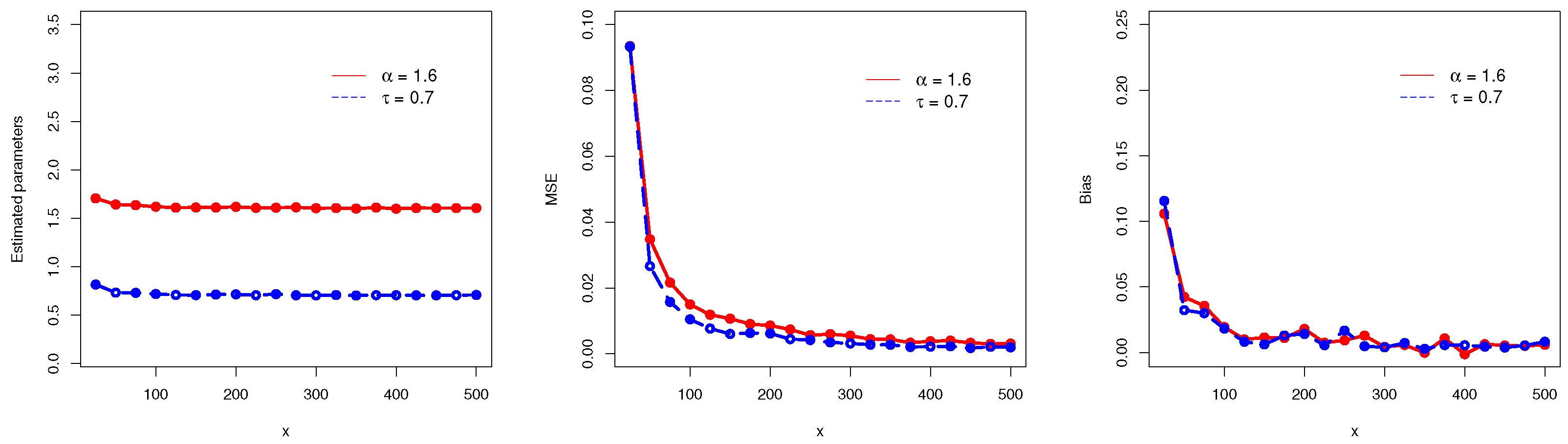
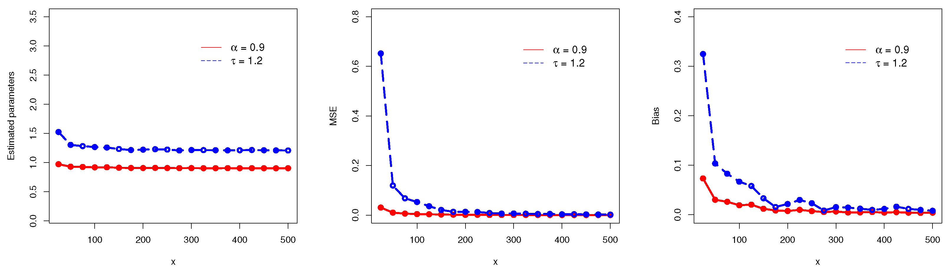
3.2. Simulation
This subsection illustrates the MLEs
of the parameters
of the NMS-Weibull distribution via a brief SS. The SS is conducted by generating random numbers from the NMS-Weibull distribution using the inverse CDF approach/formula, given by
The SS is conducted for (
i)
(
ii)
and (
iii)
Two evaluation criteria, (
i) bias and (
ii) mean square error (MSE), are considered to assess the behaviors of
and
. The values of the evaluation criteria are computed as
and
The evaluation criteria are also computed for . We use the statistical software -script with algorithm -- to compute the values of the , , and evaluation criteria.
Corresponding to (
i)
(
ii)
and (
iii)
the results of the SS of the NMS-Weibull distribution are presented in
Table 1,
Table 2 and
Table 3 (numerical results) and
Figure 3,
Figure 4 and
Figure 5 (visual illustration).
From the numerical evaluation in
Table 1,
Table 2 and
Table 3 and visual description in
Figure 3,
Figure 4 and
Figure 5, we can see that as the size of the samples increases, the MLEs
tend to become stable, the MSEs of
and
decrease, and the biases of
and
decay to zero.
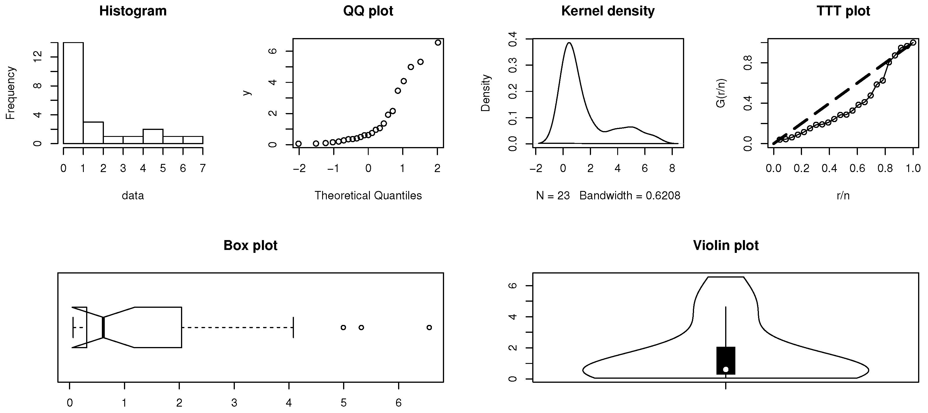
4. Data Analysis
This section is carried out with the aim of illustrating the NMS-Weibull distribution in practical scenarios, particularly in the engineering-related sectors. We apply the NMS-Weibull distribution to a reliability data set reported by [
18]. This data set denotes the times between successive failures (measured in thousands of hours) in testing secondary reactor pumps. So far, in the literature, numerous researchers have used this data set; see [
19,
20,
21]. The considered reliability data set along with its basic statistical measures are provided in
Table 4. In addition, some basic plots of the reliability data set are presented in
Figure 6.
Using the reliability data set, the comparison of the NMS-Weibull distribution is done with the Weibull model and its other prominent and most famous extensions. The SFs of the considered competing distributions are given by
Weibull distribution of Weibull [
22].
Exponential TX Weibull (ETX-Weibull) distribution of Ahmad et al. [
23].
New modified Weibull (NM-Weibull) distribution of El-Morshedy et al. [
24].
To determine the most appropriate and best-suited model from the NMS-Weibull and the above competing models, we use certain well-known decision tools (selection criteria) with the p-value. The selection criteria are as follows:
The Cramér–von Mises (CVM) criterion, computed as
where
and
n, respectively, denote the
observation and the size of the data considered for analysis.
The Anderson–Darling (AD) criterion, obtained using the formula
The Kolmogorov–Smirnov (KS) criterion, obtained as
where
and
are, respectively, called the empirical CDF and estimated CDF.
We implement the statistical software -script version with and the algorithm to calculate the values of the above selection criteria.
After analyzing the secondary reactor pumps data set, the MLEs of the fitted model
are presented in
Table 5. As we discussed in
Section 3, the MLEs
are not in explicit forms. Therefore, to check the uniqueness of
and
for the NMS-Weibull distribution, the profiles of the log-likelihood function of
and
are presented in
Figure 7.
Moreover, the numerical values of the statistical criteria (i.e., KS, CVM, AD) of the NMS-Weibull and other fitted distributions are presented in
Table 6. Additionally, the
p-value for all the fitted models is also presented in
Table 6. Based on our findings in
Table 6, it can be seen that the NMS-Weibull distribution is an appropriate and best-suited model for the engineering data set.
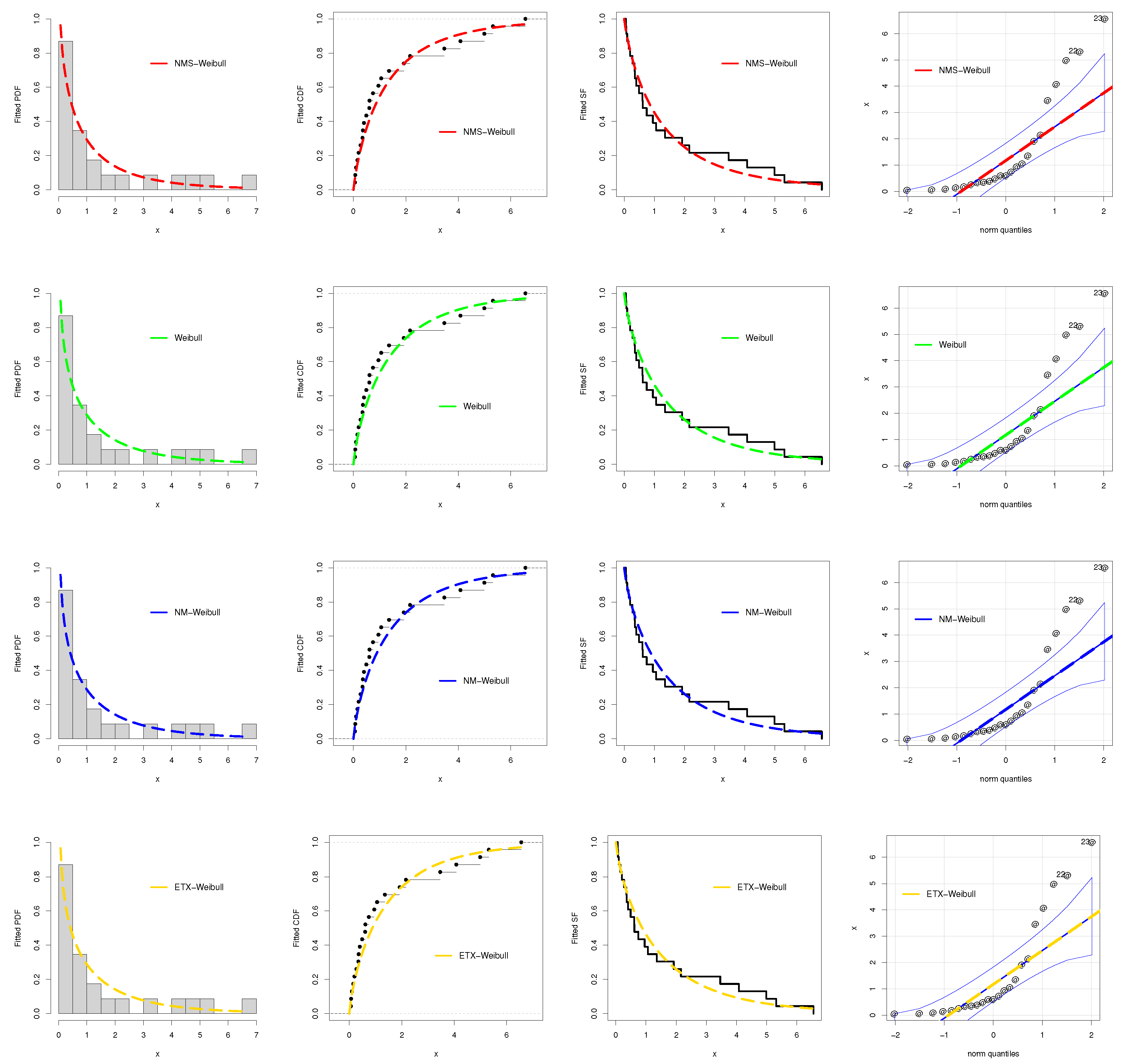
After the numerical comparison of the fitted models in
Table 6, a visual comparison of the performances of the NMS-Weibull distribution is also carried out. For the visual comparison, we consider the (
i) fitted PDF, (
ii) empirical CDF, (
iii) Kaplan Meier survival plots, and (
iv) quantile–quantile (QQ) plots. The visual comparison of these distributions is presented in
Figure 8. Based on the illustrated plots in
Figure 8, we can see that the NMS-Weibull distribution fits the failure times in the secondary reactor pumps data set very closely.
5. The Attribute Control Charts
Quality control has become a difficult undertaking in both the industrial and service sectors. The development of a reputation in highly competitive marketplaces is dependent on providing a high-quality service or product. Quality planning, assurance, and improvement are ongoing processes in every organization. The importance of statistical quality control (SQC) in the science of quality enhancement or assurance cannot be overstated. Though the use of variable and attribute control charts started in the manufacturing business, there is a growing trend of their use in the healthcare industry. Control charts, as an SQC tool, are essential for recognizing assignable reasons for variation, as well as for correcting the system and maintaining quality. Attribute control charts apply to binomial classification problems such as “confirming to the pre-specified quality” or “non-confirming”. Dutta et al. [
25] investigated the digitization priorities of quality control processes for SMEs, a conceptual study in the context of Industry 4.0 adoption. For more detail, we refer interested readers to [
26,
27,
28,
29,
30]. There are two types of control charts used in statistical quality control processes: control charts for attributes and control charts for variables. Because it uses quantitative data, the variables control chart provides useful information about the process and includes minimum sample sizes. Because of its ease of computation, the attribute control chart is more flexible than the variables chart. Various attribute control charts, such as the
np chart,
u chart, and
c chart, are well-known in the literature.
Several authors have investigated the attribute control chart for the time-truncated life test for various distributions; refer to [
31,
32,
33,
34]. Recently, Alomair et al. [
35] studied a control chart using the trigonometrically generated distribution. They studied a new trigonometric modification of the Weibull distribution, control chart, and applications in quality control.
However, there is no work on attribute control charts based on the NMS-Weibull distribution in the literature. Therefore, we use the NMS-Weibull model to project a new attribute control chart based on a truncated life test in this paper.
5.1. The Proposed Control Chart
We propose a new
np control chart based on time-truncated life testing developed by Aslam and Jun [
36]:
Step 1: Examining a simple random sample of size n from the submitted lot. The number of failures denoted by D is obtained before the experiment time , where is the quality consideration under the condition that the process is in-control and a is a multiplier constant.
Step 2: Declare the process as out-of-control when or ; otherwise, the process is in-control if
The percentile of the NMS-Weibull distribution is
From Equation (
11), we have
or
where
Using the binomial distribution of defective products with parameters
and
n, the proposed chart limits are obtained as
and
where
is the probability of a failed item prior to testing time
when the process is considered to be in-control, and
L is the chart coefficient to be obtained. On the other hand, once the process is under control, we can say it is complete
(i.e.,
and
).
Let us consider that the experiment time is
as a multiple of termination ratio
a and specified percentile life
, i.e.,
in time-truncated lifetime experimentation. After simplification, the probability of failure is written as
When the process is in-control, then the percentile ratio
. Therefore, Equation (
15) will be reduced to
Now, we consider the percentile ratio
Then, the probability in Equation (
15) becomes
Let
denote the sample’s average failure rate for the subgroups. If the value of
is unknown, the chart limits can be calculated using the following equations:
and
For the developed control chart, the possibility of declaring that the process is in-control is given by:
The developed control chart’s success can be measured by its average run length (ARL), which is expressed as follows, when the process is in-control:
The study of out-of-control processes is required to investigate the performance of the proposed control chart. When the process is out-of-control, consider
to be the probability of an unsuccessful item occurring before the experiment time
. As a result, the probability that the process is clearly in-control, while the declared time ratio is changed to
c, is given by
As a result, the ARL for the shifted process is as follows:
Monte Carlo simulations have been performed using software of version in order to evaluate the performance of the proposed control charting techniques. The following step-by-step procedure can be used to acquire the tables of the developed control chart.
Find out the ARL value, say and known parametric values and , respectively.
Determine the chart constants L, a and n such that the value is almost equal to , i.e., .
Subsequent to receiving the values in Step 2, determine the
according to shift constant
c based on Equation (
23).
For various values, we determined the control chart parameters and
at
and
n for shift values in
Table 7,
Table 8,
Table 9 and
Table 10.
5.2. Chart Illustration
The demonstration of the developed control chart is as follows: let us assume that industrial output persists in the NMS-Weibull distribution with parameters
. Assume the product’s average target lifetime is
h and
. Using Equation (
16) the value of
is 0.4887.
In addition, from
Table 7, the chart parameters are
, and
Hence, the experiment time
is 983 h. As a result, the proposed control chart was implemented as follows.
Take a simple random sample of 20 people from each subgroup and place them in the life testing assessment for 983 h. Determine the number of failed units, say D, over the course of the experiment.
If is present, the production process is under control; otherwise, the production process is out of control.
5.3. Application in Industry
Using the second data set, the estimated parameters of the NMS-Weibull distribution are
and
Table 11 and
Table 12 show the ARLs of the proposed control chart for failure times in the secondary reactor pumps data set.
From
Table 11, for
n = 20,
, we get
and
The value of
is 0.4719 using Equation (
16). According to Equation (
16), the median value
for the test’s duration is 0.8498. The suggested control limits for the chart are LCL = 0 and UCL = 5.1210. The proposed control chart for the failure times in the secondary reactor pumps data is depicted in
Figure 9. Using the same data, the estimates of the Weibull distribution parameters are
and
When
and
, we get
and
The control limits for the Weibull distribution are LCL = 0 and UCL = 5.3501. The control chart for failure times in the secondary reactor pump data for the Weibull distribution is depicted in
Figure 10. As seen in
Figure 9 and
Figure 10, the suggested chart for detecting data on the failure times between secondary reactor pumps is more accurate than the existing attribute control chart for the Weibull distribution. As a result, the suggested chart is appropriate for tracking the reliability of secondary reactor pumps failure data.
5.4. Comparison
The ARL values of the proposed control chart and the existing time-truncated life testing attributed control charts for the Weibull distribution given in Adeoti and Rao [
37] are compared. The results of comparisons between the NMS-Weibull distribution and the Weibull distribution are displayed in
Table 13, when
and
To compare the two types of control charts with respect to ARL values at different shift values, it is important to note that a chart with fewer out-of-control ARLs would be considered the better control chart.
We noticed based on
Table 7 that the ARL values of the developed control chart have fever ARLs as compared with the control chart developed for Weibull distribution. For instance, when
c = 1.4, the
of the developed NMS-Weibull control chart for
n = 20 is 100.52, whereas the
for the Weibull distribution is 107.48. Hence, we conclude that the proposed chart is quick to find process changes as compared with the existing control chart established on the Weibull distribution.
6. Limitations of the Study
Despite the advantage of the best-fitting ability and distributional flexibility of capturing different forms of the density function, the NMS-Weibull distribution also has certain limitations. The NMS-Weibull distribution has the following limitations:
Since the NMS-Weibull distribution is a continuous type distribution, it would not be a sensible decision to use it for modeling discrete-type data sets.
Due to the complicated form of the density function, more computational effort is needed to obtain the distributional properties of the NMS-Weibull distribution.
Due to the complicated form of the density function, the expressions for the MLEs of the NMS-Weibull distribution are not in explicit forms. Therefore, we need to use computer software to obtain the numerical estimates for the parameters of the NMS-Weibull distribution.
7. Concluding Remarks
In this paper, we proposed a novel method by incorporating a trigonometric function to update the distributional flexibility of the classical probability distributions. The proposed method was named a new modified sine-G approach. The new modified sine-G method was developed using the sine function. As a special member of the NMS-G method, a new sine-Weibull distribution was studied. The parameters of the NMS-Weibull distribution were estimated using the maximum likelihood estimation method. A simulation study was also conducted to evaluate the estimators of the NMS-Weibull distribution. A practical application of the proposed NMS-Weibull distribution in the industrial sector was considered. In addition, the attribute control chart was developed for the proposed distribution. The control chart limits were developed for various parametric combinations. The performance of the proposed control charts was studied in terms of ARLs for various shift values. The developed control chart was also illustrated with a real example.
Author Contributions
Conceptualization, H.M.A., G.S.R., J.-T.S. and S.K.K.; methodology, H.M.A., G.S.R., J.-T.S. and S.K.K.; software, H.M.A., G.S.R., J.-T.S. and S.K.K.; validation, H.M.A., G.S.R. and J.-T.S.; formal analysis, H.M.A., G.S.R., J.-T.S. and S.K.K.; investigation, H.M.A., J.-T.S. and S.K.K.; data curation, H.M.A. and S.K.K.; writing—original draft, H.M.A., G.S.R., J.-T.S. and S.K.K.; visualization, H.M.A., G.S.R., J.-T.S. and S.K.K. All authors have read and agreed to the published version of the manuscript.
Funding
Princess Nourah bint Abdulrahman University Researchers Supporting Project number (PNURSP2023R 299), Princess Nourah bint Abdulrahman University, Riyadh, Saudi Arabia.
Data Availability Statement
The data sets are available from the corresponding author upon request.
Conflicts of Interest
The authors declare no competing interests.
References
- Alotaibi, R.; Nassar, M.; Rezk, H.; Elshahhat, A. Inferences and engineering applications of alpha power Weibull distribution using progressive type-II censoring. Mathematics 2022, 10, 2901. [Google Scholar] [CrossRef]
- Alyami, S.A.; Elbatal, I.; Alotaibi, N.; Almetwally, E.M.; Okasha, H.M.; Elgarhy, M. Topp–Leone Modified Weibull Model: Theory and Applications to Medical and Engineering Data. Appl. Sci. 2022, 12, 10431. [Google Scholar] [CrossRef]
- Klakattawi, H.S. Survival analysis of cancer patients using a new extended Weibull distribution. PLoS ONE 2022, 17, e0264229. [Google Scholar] [CrossRef]
- Ahmad, Z.; Almaspoor, Z.; Khan, F.; El-Morshedy, M. On predictive modeling using a new flexible Weibull distribution and machine learning approach: Analyzing the COVID-19 data. Mathematics 2022, 10, 1792. [Google Scholar] [CrossRef]
- Silahli, B.; Dingec, K.D.; Cifter, A.; Aydin, N. Portfolio value-at-risk with two-sided Weibull distribution: Evidence from cryptocurrency markets. Financ. Res. Lett. 2021, 38, 101425. [Google Scholar] [CrossRef]
- Ahmad, Z.; Almaspoor, Z.; Khan, F.; Alhazmi, S.E.; El-Morshedy, M.; Ababneh, O.Y.; Al-Omari, A.I. On fitting and forecasting the log-returns of cryptocurrency exchange rates using a new logistic model and machine learning algorithms. AIMS Math. 2022, 7, 18031–18049. [Google Scholar] [CrossRef]
- Barthwal, A.; Acharya, D. Performance analysis of sensing-based extreme value models for urban air pollution peaks. Model. Earth Syst. Environ. 2022, 8, 4149–4163. [Google Scholar] [CrossRef]
- Natarajan, N.; Vasudevan, M.; Rehman, S. Evaluation of suitability of wind speed probability distribution models: A case study from Tamil Nadu, India. Environ. Sci. Pollut. Res. 2022, 29, 85855–85868. [Google Scholar] [CrossRef]
- El-Morshedy, M.; Eliwa, M.S.; Tyagi, A. A discrete analogue of odd Weibull-G family of distributions: Properties, classical and Bayesian estimation with applications to count data. J. Appl. Stat. 2022, 49, 2928–2952. [Google Scholar] [CrossRef]
- Eghwerido, J.T.; Agu, F.I.; Ibidoja, O.J. The shifted exponential-G family of distributions: Properties and applications. J. Stat. Manag. Syst. 2022, 25, 43–75. [Google Scholar] [CrossRef]
- Anzagra, L.; Sarpong, S.; Nasiru, S. Odd Chen-G family of distributions. Ann. Data Sci. 2022, 9, 369–391. [Google Scholar] [CrossRef]
- Hassan, A.S.; Al-Omari, A.I.; Hassan, R.R.; Alomani, G.A. The odd inverted Topp Leone–H family of distributions: Estimation and applications. J. Radiat. Res. Appl. Sci. 2022, 15, 365–379. [Google Scholar] [CrossRef]
- Chesneau, C.; Bakouch, H.S.; Hussain, T. A new class of probability distributions via cosine and sine functions with applications. Commun. Stat. Simul. Comput. 2019, 48, 2287–2300. [Google Scholar] [CrossRef]
- Kumar, D.; Singh, U.; Singh, S.K. A new distribution using sine function-its application to bladder cancer patients data. J. Stat. Appl. Probab. 2015, 4, 417. [Google Scholar]
- Chesneau, C.; Jamal, F. The sine Kumaraswamy-G family of distributions. J. Math. Ext. 2020, 15, 1–33. [Google Scholar]
- Al-Babtain, A.A.; Elbatal, I.; Chesneau, C.; Elgarhy, M. Sine Topp-Leone-G family of distributions: Theory and applications. Open Phys. 2020, 18, 574–593. [Google Scholar] [CrossRef]
- Jamal, F.; Chesneau, C.; Bouali, D.L.; Ul Hassan, M. Beyond the Sin-G family: The transformed Sin-G family. PLoS ONE 2021, 16, e0250790. [Google Scholar] [CrossRef]
- Suprawhardana, M.S.; Prayoto, S. Total time on test plot analysis for mechanical components of the RSG-GAS reactor. Atom Indones. 1999, 25, 81–90. [Google Scholar]
- Bebbington, M.; Lai, C.D.; Zitikis, R. A flexible Weibull extension. Reliab. Eng. Syst. Saf. 2007, 92, 719–726. [Google Scholar] [CrossRef]
- Coşkun, K.U.Ş.; Korkmaz, M.Ç.; Kinaci, İ.; Karakaya, K.; Akdogan, Y. Modified-Lindley distribution and its applications to the real data. Commun. Fac. Sci. Univ. Ank. Ser. Math. Stat. 2022, 71, 252–272. [Google Scholar]
- Demirci Bicer, H.; Bicer, C.; Bakouch, H.S.H. A geometric process with Hjorth marginal: Estimation, discrimination, and reliability data modeling. Qual. Reliab. Eng. Int. 2022, 38, 2795–2819. [Google Scholar] [CrossRef]
- Weibull, W. A Statistical Distribution of wide Applicability. J. Appl. Mech. 1951, 18, 239–296. [Google Scholar] [CrossRef]
- Ahmad, Z.; Mahmoudi, E.; Alizadeh, M.; Roozegar, R.; Afify, A.Z. The exponential TX family of distributions: Properties and an application to insurance data. J. Math. 2021, 2021, 3058170. [Google Scholar] [CrossRef]
- El-Morshedy, M.; Ahmad, Z.; Tag-Eldin, E.; Almaspoor, Z.; Eliwa, M.S.; Iqbal, Z. A new statistical approach for modeling the bladder cancer and leukemia patients data sets: Case studies in the medical sector. Math. Biosci. Eng. MBE 2022, 19, 10474–10492. [Google Scholar] [CrossRef]
- Dutta, G.; Kumar, R.; Sindhwani, R.; Singh, R.K. Digitalization priorities of quality control processes for SMEs: A conceptual study in perspective of Industry 4.0 adoption. J. Intell. Manuf. 2021, 32, 1679–1698. [Google Scholar] [CrossRef]
- Meramveliotakis, G.; Manioudis, M. Sustainable development, COVID-19 and small business in Greece: Small is not beautiful. Adm. Sci. 2021, 11, 90. [Google Scholar] [CrossRef]
- Moeuf, A.; Pellerin, R.; Lamouri, S.; Tamayo-Giraldo, S.; Barbaray, R. The industrial management of SMEs in the era of Industry 4.0. Int. J. Prod. Res. 2018, 56, 1118–1136. [Google Scholar] [CrossRef]
- Kahar, A.; Tampang, T.; Masdar, R.; Masrudin, M. Value chain analysis of total quality control, quality performance and competitive advantage of agricultural SMEs. Uncertain Supply Chain Manag. 2022, 10, 551–558. [Google Scholar] [CrossRef]
- Yang, C.C. The effectiveness analysis of the practices in five quality management stages for SMEs. Total. Qual. Manag. Bus. Excell. 2020, 31, 955–977. [Google Scholar] [CrossRef]
- Sundaram, S.; Zeid, A. Artificial intelligence-based smart quality inspection for manufacturing. Micromachines 2023, 14, 570. [Google Scholar] [CrossRef]
- Adeoti, O.A.; Ogundipe, P. A control chart for the generalized exponential distribution under time truncated life test. Life Cycle Reliab. Saf. Eng. 2021, 10, 53–59. [Google Scholar] [CrossRef]
- Quinino, R.D.C.; Ho, L.L.; Cruz, F.R.B.D.; Bessegato, L.F. A control chart to monitor the process mean based on inspecting attributes using control limits of the traditional X-bar chart. J. Stat. Comput. Simul. 2020, 90, 1639–1660. [Google Scholar] [CrossRef]
- Rao, G.S. A control chart for time truncated life tests using exponentiated half logistic distribution. Appl. Math. Inf. Sci. 2018, 12, 125–131. [Google Scholar] [CrossRef]
- Rao, G.S.; Al-Omari, A.I. Attribute Control Charts Based on TLT for Length-Biased Weighted Lomax Distribution. J. Math. 2022, 2022, 3091850. [Google Scholar]
- Alomair, M.A.; Ahmad, Z.; Rao, G.S.; Al-Mofleh, H.; Khosa, S.K.; Al Naim, A.S. A new trigonometric modification of the Weibull distribution: Control chart and applications in quality control. PLoS ONE 2023, 18, e0286593. [Google Scholar] [CrossRef]
- Aslam, M.; Jun, C.H. Attribute control charts for the Weibull distribution under truncated life tests. Qual. Eng. 2015, 27, 283–288. [Google Scholar] [CrossRef]
- Adeoti, O.A.; Rao, G.S. Attribute Control Chart for Rayleigh Distribution Using Repetitive Sampling under Truncated Life Test. J. Probab. Stat. 2022, 2022, 8763091. [Google Scholar] [CrossRef]
Figure 1.
Graphical illustrations of and of the NMS-Weibull distribution.
Figure 1.
Graphical illustrations of and of the NMS-Weibull distribution.
Figure 2.
Visual illustrations of of the NMS-Weibull distribution.
Figure 2.
Visual illustrations of of the NMS-Weibull distribution.
Figure 3.
Graphical illustration of the SS of the NMS-Weibull model for and .
Figure 3.
Graphical illustration of the SS of the NMS-Weibull model for and .
Figure 4.
Graphical illustration of the SS of the NMS-Weibull model for and .
Figure 4.
Graphical illustration of the SS of the NMS-Weibull model for and .
Figure 5.
Graphical illustration of the SS of the NMS-Weibull model for and .
Figure 5.
Graphical illustration of the SS of the NMS-Weibull model for and .
Figure 6.
Visual description of the failure times in the secondary reactor pumps data set.
Figure 6.
Visual description of the failure times in the secondary reactor pumps data set.
Figure 7.
The profiles of the log-likelihood function of and of the NMS-Weibull distribution.
Figure 7.
The profiles of the log-likelihood function of and of the NMS-Weibull distribution.
Figure 8.
The visual comparison of the fitted models using the failure times between secondary reactor pumps.
Figure 8.
The visual comparison of the fitted models using the failure times between secondary reactor pumps.
Figure 9.
The proposed control chart for real data.
Figure 9.
The proposed control chart for real data.
Figure 10.
The attribute control chart for Weibull distribution using real data.
Figure 10.
The attribute control chart for Weibull distribution using real data.
Table 1.
Numerical results of the SS of the NMS-Weibull for and .
Table 1.
Numerical results of the SS of the NMS-Weibull for and .
| n | Parameters | MLEs | MSEs | Biases |
|---|
| 25 | | 1.7058470 | 0.093483043 | 0.105846584 |
| 0.8155479 | 0.093283376 | 0.115547865 |
| 50 | | 1.6423630 | 0.034815198 | 0.042363078 |
| 0.7323058 | 0.026648979 | 0.032305759 |
| 75 | | 1.6355490 | 0.021650251 | 0.035549066 |
| 0.7300049 | 0.015752197 | 0.030004944 |
| 100 | | 1.6193810 | 0.015016547 | 0.019380712 |
| 0.7182018 | 0.010479930 | 0.018201807 |
| 150 | | 1.6114620 | 0.010681263 | 0.011461775 |
| 0.7062099 | 0.006044519 | 0.006209865 |
| 200 | | 1.6179430 | 0.008579487 | 0.017942898 |
| 0.7142004 | 0.006189921 | 0.014200418 |
| 250 | | 1.6093060 | 0.005664633 | 0.009306357 |
| 0.7166943 | 0.004182348 | 0.016694310 |
| 300 | | 1.6042410 | 0.005519344 | 0.004240543 |
| 0.7039717 | 0.003150546 | 0.003971737 |
| 350 | | 1.5998330 | 0.004396528 | −0.000167242 |
| 0.7027976 | 0.002760748 | 0.002797628 |
| 400 | | 1.5987060 | 0.003819449 | −0.001293900 |
| 0.7055447 | 0.002180982 | 0.005544683 |
| 450 | | 1.6053810 | 0.003354506 | 0.005381075 |
| 0.7037944 | 0.001758227 | 0.003794365 |
| 500 | | 1.6059350 | 0.003114073 | 0.005934558 |
| 0.7082324 | 0.001967812 | 0.008232406 |
Table 2.
Numerical results of the SS of the NMS-Weibull for and .
Table 2.
Numerical results of the SS of the NMS-Weibull for and .
| n | Parameters | MLEs | MSEs | Biases |
|---|
| 25 | | 1.2549060 | 0.044395238 | 0.054906051 |
| 0.5550671 | 0.027588079 | 0.055067128 |
| 50 | | 1.2358190 | 0.021338634 | 0.035818576 |
| 0.5311935 | 0.011947412 | 0.031193494 |
| 75 | | 1.2124500 | 0.011271706 | 0.012449877 |
| 0.5088994 | 0.005170900 | 0.008899357 |
| 100 | | 1.2281550 | 0.009815668 | 0.028154642 |
| 0.5175243 | 0.005363298 | 0.017524305 |
| 150 | | 1.2064990 | 0.005320626 | 0.006499179 |
| 0.5040655 | 0.002577040 | 0.004065460 |
| 200 | | 1.2035030 | 0.004052304 | 0.003503492 |
| 0.5068780 | 0.001901467 | 0.006877954 |
| 250 | | 1.2059680 | 0.003226839 | 0.005967537 |
| 0.5065202 | 0.001631163 | 0.006520181 |
| 300 | | 1.2042540 | 0.002601533 | 0.004254301 |
| 0.5037654 | 0.001372364 | 0.003765379 |
| 350 | | 1.2060550 | 0.002405026 | 0.006055456 |
| 0.5010220 | 0.001003504 | 0.001021994 |
| 400 | | 1.2068830 | 0.001971411 | 0.006882850 |
| 0.5023243 | 0.000843874 | 0.002324347 |
| 450 | | 1.2059420 | 0.002005009 | 0.005941682 |
| 0.5024952 | 0.000792774 | 0.002495189 |
| 500 | | 1.2032020 | 0.001486821 | 0.003202500 |
| 0.5009489 | 0.000760580 | 0.000948948 |
Table 3.
Numerical results of the SS of the NMS-Weibull for and .
Table 3.
Numerical results of the SS of the NMS-Weibull for and .
| n | Parameters | MLEs | MSEs | Biases |
|---|
| 25 | | 0.9731610 | 0.030667641 | 0.073161002 |
| 1.5246250 | 0.651926648 | 0.324624826 |
| 50 | | 0.9300565 | 0.010075393 | 0.030056496 |
| 1.3033900 | 0.119277460 | 0.103390382 |
| 75 | | 0.9259897 | 0.006206455 | 0.025989684 |
| 1.2826580 | 0.067869132 | 0.082657543 |
| 100 | | 0.9190743 | 0.004337160 | 0.019074256 |
| 1.2666830 | 0.052836251 | 0.066682575 |
| 150 | | 0.9118796 | 0.002542578 | 0.011879576 |
| 1.2330440 | 0.021079314 | 0.033043678 |
| 200 | | 0.9074134 | 0.001198230 | 0.007413419 |
| 1.2214930 | 0.013374842 | 0.021492592 |
| 250 | | 0.9072119 | 0.001005603 | 0.007211943 |
| 1.2230720 | 0.008603171 | 0.023071959 |
| 300 | | 0.9063632 | 0.000802679 | 0.006363228 |
| 1.2152340 | 0.006835559 | 0.015233889 |
| 350 | | 0.9045964 | 0.000531511 | 0.004596404 |
| 1.2120730 | 0.004612884 | 0.012072942 |
| 400 | | 0.9040632 | 0.000349953 | 0.004063192 |
| 1.2115680 | 0.003378131 | 0.011567549 |
| 450 | | 0.9039290 | 0.000319477 | 0.003928996 |
| 1.2115500 | 0.002911736 | 0.011550037 |
| 500 | | 0.9039453 | 0.000274294 | 0.003945275 |
| 1.2078420 | 0.002132846 | 0.007841758 |
Table 4.
The failure times in the secondary reactor pumps data set with summary values.
Table 4.
The failure times in the secondary reactor pumps data set with summary values.
| 2.160, 0.746, 0.402, 0.954, 0.491, 6.560, 4.992, 0.347, 0.150, 0.358, 0.101, 1.359, |
|---|
| 3.465, 1.060, 0.614, 1.921, 4.082, 0.199, 0.605, 0.273, 0.070, 0.062, 5.320 |
| n | Min. | Max. | | Median | |
| 23 | 0.062 | 6.560 | 1.578 | 0.614 | 3.7275 |
| | | Skewness | Kurtosis | Range |
| 0.310 | 1.9306 | 2.041 | 1.3643 | 3.54453 | 6.498 |
Table 5.
Using the failure times between secondary reactor pumps, the values of , and of the fitted distributions.
Table 5.
Using the failure times between secondary reactor pumps, the values of , and of the fitted distributions.
| Models | | | | |
|---|
| NMS-Weibull | 0.8623 | 0.1338 | - | - |
| Weibull | 0.8091 | 0.7642 | - | - |
| NM-Weibull | 0.8000 | 0.7835 | 26.5708 | - |
| ETX-Weibull | 0.8009 | 26.7728 | - | 0.79023 |
Table 6.
For the failure times between secondary reactor pumps, the values of the selection criteria of the fitted distributions.
Table 6.
For the failure times between secondary reactor pumps, the values of the selection criteria of the fitted distributions.
| Models | CVM | AD | KS | p-Value |
|---|
| NMS-Weibull | 0.0578 | 0.3908 | 0.1101 | 0.9143 |
| Weibull | 0.0655 | 0.4315 | 0.1192 | 0.8615 |
| NM-Weibull | 0.0662 | 0.4353 | 0.1192 | 0.8614 |
| ETX-Weibull | 0.0664 | 0.4365 | 0.1168 | 0.8766 |
Table 7.
The ARLs values of the proposed chart for and .
Table 7.
The ARLs values of the proposed chart for and .
| 200 | 250 | 300 | 370 | 500 |
|---|
| 2.884 | 2.955 | 2.938 | 3.03 | 3.158 |
| 0.879 | 0.808 | 0.958 | 0.983 | 0.846 |
| | | | | |
| 0.10 | 1.00 | 1.00 | 1.00 | 1.00 | 1.00 |
| 0.20 | 1.01 | 1.01 | 1.01 | 1.02 | 1.01 |
| 0.30 | 1.19 | 1.22 | 1.17 | 1.34 | 1.30 |
| 0.40 | 1.96 | 2.08 | 1.87 | 2.60 | 2.44 |
| 0.50 | 4.16 | 4.49 | 3.88 | 6.46 | 5.83 |
| 0.60 | 9.93 | 10.75 | 9.17 | 17.86 | 15.33 |
| 0.70 | 24.74 | 26.58 | 22.88 | 50.95 | 41.33 |
| 0.80 | 60.95 | 64.75 | 57.63 | 141.44 | 109.48 |
| 0.85 | 92.79 | 98.76 | 90.77 | 223.52 | 174.27 |
| 0.90 | 134.06 | 145.40 | 140.87 | 319.88 | 268.23 |
| 0.95 | 175.98 | 200.81 | 212.04 | 343.54 | 387.12 |
| 1.00 | 200.70 | 250.51 | 300.44 | 370.44 | 500.27 |
| 1.05 | 196.47 | 241.17 | 282.97 | 302.71 | 485.51 |
| 1.10 | 170.84 | 233.97 | 242.29 | 227.89 | 449.46 |
| 1.15 | 139.02 | 211.35 | 198.58 | 167.79 | 412.00 |
| 1.20 | 110.25 | 192.39 | 183.70 | 124.31 | 364.17 |
| 1.25 | 87.18 | 156.57 | 169.81 | 93.68 | 287.37 |
| 1.30 | 69.50 | 126.98 | 151.03 | 72.01 | 226.58 |
| 1.40 | 45.91 | 85.26 | 120.05 | 45.11 | 144.99 |
| 1.50 | 32.01 | 59.74 | 84.04 | 30.26 | 97.61 |
| 1.60 | 23.40 | 43.68 | 57.28 | 21.48 | 68.98 |
| 1.70 | 17.82 | 33.15 | 40.93 | 15.97 | 50.81 |
| 1.80 | 14.03 | 25.97 | 30.45 | 12.34 | 38.78 |
| 1.90 | 11.36 | 20.91 | 23.45 | 9.84 | 30.49 |
| 2.00 | 9.43 | 17.22 | 18.58 | 8.07 | 24.58 |
| 3.00 | 3.15 | 5.25 | 4.66 | 2.60 | 6.56 |
| 4.00 | 1.97 | 3.03 | 2.55 | 1.67 | 3.54 |
Table 8.
The ARL values of the proposed chart for and .
Table 8.
The ARL values of the proposed chart for and .
| 200 | 250 | 300 | 370 | 500 |
|---|
| 2.888 | 2.953 | 4.125 | 3.033 | 3.48 |
| 0.843 | 0.752 | 0.546 | 0.978 | 0.623 |
| | | | | |
| 0.10 | 1.00 | 1.00 | 1.00 | 1.00 | 1.00 |
| 0.20 | 1.01 | 1.01 | 1.15 | 1.02 | 1.03 |
| 0.30 | 1.19 | 1.22 | 2.39 | 1.34 | 1.50 |
| 0.40 | 1.95 | 2.09 | 7.29 | 2.60 | 3.21 |
| 0.50 | 4.13 | 4.51 | 24.52 | 6.43 | 8.24 |
| 0.60 | 9.84 | 10.82 | 80.82 | 17.75 | 22.32 |
| 0.70 | 24.47 | 26.77 | 163.07 | 50.61 | 59.85 |
| 0.80 | 60.20 | 65.26 | 195.59 | 140.42 | 152.22 |
| 0.85 | 91.69 | 99.54 | 210.22 | 222.05 | 232.16 |
| 0.90 | 132.66 | 146.48 | 242.30 | 318.38 | 333.59 |
| 0.95 | 174.75 | 202.02 | 279.98 | 343.04 | 435.84 |
| 1.00 | 200.31 | 251.41 | 300.69 | 371.34 | 501.33 |
| 1.05 | 197.10 | 234.31 | 236.65 | 304.21 | 475.10 |
| 1.10 | 172.03 | 223.36 | 187.87 | 229.29 | 458.56 |
| 1.15 | 140.28 | 213.35 | 151.21 | 168.89 | 390.96 |
| 1.20 | 111.35 | 191.34 | 123.54 | 125.12 | 323.76 |
| 1.25 | 88.08 | 155.64 | 102.41 | 94.27 | 265.88 |
| 1.30 | 70.21 | 126.20 | 86.04 | 72.45 | 218.90 |
| 1.40 | 46.35 | 84.75 | 62.95 | 45.37 | 152.08 |
| 1.50 | 32.29 | 59.40 | 47.97 | 30.42 | 109.92 |
| 1.60 | 23.60 | 43.44 | 37.79 | 21.58 | 82.47 |
| 1.70 | 17.95 | 32.98 | 30.61 | 16.04 | 63.92 |
| 1.80 | 14.13 | 25.85 | 25.37 | 12.38 | 50.92 |
| 1.90 | 11.44 | 20.81 | 21.44 | 9.88 | 41.53 |
| 2.00 | 9.49 | 17.15 | 18.43 | 8.09 | 34.56 |
| 3.00 | 3.16 | 5.24 | 7.03 | 2.61 | 10.73 |
| 4.00 | 1.98 | 3.02 | 4.33 | 1.67 | 5.95 |
Table 9.
The ARL values of the proposed chart for and .
Table 9.
The ARL values of the proposed chart for and .
| 200 | 250 | 300 | 370 | 500 |
|---|
| 2.907 | 2.992 | 2.971 | 2.981 | 3.123 |
| 0.906 | 0.809 | 0.673 | 0.906 | 0.698 |
| | | | | |
| 0.10 | 1.00 | 1.00 | 1.00 | 1.00 | 1.00 |
| 0.20 | 1.00 | 1.00 | 1.00 | 1.00 | 1.00 |
| 0.30 | 1.02 | 1.04 | 1.09 | 1.06 | 1.10 |
| 0.40 | 1.29 | 1.37 | 1.64 | 1.56 | 1.74 |
| 0.50 | 2.26 | 2.55 | 3.39 | 3.39 | 3.83 |
| 0.60 | 5.12 | 5.95 | 8.29 | 9.40 | 10.09 |
| 0.70 | 13.40 | 15.63 | 21.78 | 29.44 | 28.48 |
| 0.80 | 37.41 | 43.04 | 57.87 | 95.61 | 81.29 |
| 0.85 | 62.56 | 71.33 | 93.19 | 168.17 | 135.87 |
| 0.90 | 102.06 | 116.09 | 146.59 | 273.11 | 222.43 |
| 0.95 | 154.83 | 180.09 | 219.82 | 367.05 | 348.48 |
| 1.00 | 201.33 | 251.90 | 301.85 | 370.65 | 500.69 |
| 1.05 | 189.38 | 226.81 | 289.43 | 294.45 | 423.67 |
| 1.10 | 178.12 | 207.36 | 272.73 | 209.52 | 381.51 |
| 1.15 | 135.64 | 200.07 | 246.91 | 145.83 | 365.05 |
| 1.20 | 99.68 | 186.32 | 231.56 | 102.93 | 339.66 |
| 1.25 | 73.41 | 141.45 | 227.22 | 74.48 | 308.30 |
| 1.30 | 54.98 | 107.73 | 181.75 | 55.35 | 295.86 |
| 1.40 | 32.84 | 65.27 | 118.42 | 32.89 | 185.22 |
| 1.50 | 21.23 | 42.28 | 80.74 | 21.24 | 122.12 |
| 1.60 | 14.68 | 29.09 | 57.65 | 14.68 | 84.73 |
| 1.70 | 10.71 | 21.04 | 42.88 | 10.71 | 61.44 |
| 1.80 | 8.18 | 15.87 | 33.00 | 8.18 | 46.25 |
| 1.90 | 6.48 | 12.40 | 26.15 | 6.48 | 35.92 |
| 2.00 | 5.29 | 9.98 | 21.24 | 5.29 | 28.66 |
| 3.00 | 1.83 | 2.89 | 5.95 | 1.83 | 7.17 |
| 4.00 | 1.29 | 1.77 | 3.30 | 1.29 | 3.76 |
Table 10.
The ARL values of the proposed chart for and .
Table 10.
The ARL values of the proposed chart for and .
| 200 | 250 | 300 | 370 | 500 |
|---|
| 2.905 | 2.991 | 2.939 | 3.1 | 3.122 |
| 0.877 | 0.754 | 0.932 | 0.905 | 0.619 |
| | | | | |
| 0.10 | 1.00 | 1.00 | 1.00 | 1.00 | 1.00 |
| 0.20 | 1.00 | 1.00 | 1.00 | 1.00 | 1.00 |
| 0.30 | 1.02 | 1.04 | 1.02 | 1.04 | 1.10 |
| 0.40 | 1.28 | 1.37 | 1.30 | 1.41 | 1.74 |
| 0.50 | 2.26 | 2.54 | 2.32 | 2.75 | 3.84 |
| 0.60 | 5.11 | 5.94 | 5.37 | 6.95 | 10.11 |
| 0.70 | 13.35 | 15.59 | 14.47 | 20.13 | 28.56 |
| 0.80 | 37.23 | 42.91 | 41.83 | 61.71 | 81.57 |
| 0.85 | 62.26 | 71.10 | 71.70 | 107.87 | 136.35 |
| 0.90 | 101.59 | 115.73 | 121.89 | 183.26 | 223.20 |
| 0.95 | 154.25 | 179.59 | 200.31 | 286.00 | 349.58 |
| 1.00 | 200.97 | 250.42 | 300.42 | 370.81 | 500.90 |
| 1.05 | 189.56 | 291.67 | 285.00 | 359.57 | 474.37 |
| 1.10 | 178.63 | 287.63 | 267.04 | 296.68 | 451.27 |
| 1.15 | 136.17 | 240.53 | 246.01 | 214.97 | 434.17 |
| 1.20 | 100.10 | 186.77 | 217.59 | 152.15 | 418.62 |
| 1.25 | 73.72 | 141.81 | 156.31 | 108.83 | 377.37 |
| 1.30 | 55.20 | 108.00 | 113.24 | 79.57 | 295.10 |
| 1.40 | 32.96 | 65.43 | 63.17 | 45.70 | 184.76 |
| 1.50 | 21.31 | 42.38 | 38.38 | 28.60 | 121.83 |
| 1.60 | 14.72 | 29.15 | 25.11 | 19.22 | 84.54 |
| 1.70 | 10.74 | 21.08 | 17.47 | 13.69 | 61.32 |
| 1.80 | 8.20 | 15.90 | 12.78 | 10.23 | 46.16 |
| 1.90 | 6.49 | 12.42 | 9.74 | 7.95 | 35.86 |
| 2.00 | 5.31 | 9.99 | 7.70 | 6.38 | 28.61 |
| 3.00 | 1.83 | 2.90 | 2.17 | 1.99 | 7.16 |
| 4.00 | 1.29 | 1.77 | 1.40 | 1.34 | 3.75 |
Table 11.
The ARL values of the proposed chart for and .
Table 11.
The ARL values of the proposed chart for and .
| 200 | 250 | 300 | 370 | 500 |
|---|
| 2.891 | 2.953 | 2.939 | 3.059 | 3.157 |
| 0.744 | 0.609 | 0.905 | 0.864 | 0.678 |
| | | | | |
| 0.10 | 1.00 | 1.00 | 1.00 | 1.00 | 1.00 |
| 0.20 | 1.01 | 1.01 | 1.01 | 1.01 | 1.01 |
| 0.30 | 1.18 | 1.22 | 1.17 | 1.21 | 1.30 |
| 0.40 | 1.95 | 2.09 | 1.87 | 2.08 | 2.45 |
| 0.50 | 4.11 | 4.51 | 3.88 | 4.59 | 5.84 |
| 0.60 | 9.77 | 10.83 | 9.18 | 11.45 | 15.39 |
| 0.70 | 24.28 | 26.79 | 22.92 | 29.86 | 41.51 |
| 0.80 | 59.71 | 65.32 | 57.74 | 77.76 | 110.00 |
| 0.85 | 90.95 | 99.62 | 90.95 | 123.64 | 175.11 |
| 0.90 | 131.73 | 146.59 | 141.15 | 191.40 | 269.46 |
| 0.95 | 173.91 | 202.15 | 212.45 | 280.32 | 388.59 |
| 1.00 | 200.02 | 251.51 | 300.91 | 370.36 | 500.42 |
| 1.05 | 197.51 | 234.32 | 283.33 | 339.73 | 455.68 |
| 1.10 | 172.83 | 213.29 | 221.32 | 313.00 | 428.63 |
| 1.15 | 141.14 | 203.25 | 198.29 | 301.50 | 410.73 |
| 1.20 | 112.10 | 191.23 | 167.27 | 270.75 | 362.91 |
| 1.25 | 88.68 | 155.54 | 159.39 | 209.65 | 286.30 |
| 1.30 | 70.69 | 126.12 | 140.68 | 162.26 | 225.72 |
| 1.40 | 46.65 | 84.70 | 129.83 | 100.52 | 144.45 |
| 1.50 | 32.49 | 59.36 | 83.91 | 65.97 | 97.28 |
| 1.60 | 23.73 | 43.42 | 57.19 | 45.71 | 68.75 |
| 1.70 | 18.05 | 32.97 | 40.87 | 33.17 | 50.66 |
| 1.80 | 14.20 | 25.84 | 30.41 | 25.03 | 38.67 |
| 1.90 | 11.49 | 20.80 | 23.42 | 19.51 | 30.40 |
| 2.00 | 9.53 | 17.14 | 18.56 | 15.64 | 24.52 |
| 3.00 | 3.17 | 5.24 | 4.65 | 4.21 | 6.55 |
| 4.00 | 1.98 | 3.02 | 2.54 | 2.38 | 3.53 |
Table 12.
The ARL values of the proposed chart for and .
Table 12.
The ARL values of the proposed chart for and .
| 200 | 250 | 300 | 370 | 500 |
|---|
| 2.901 | 2.99 | 2.941 | 3.099 | 3.144 |
| 0.797 | 0.612 | 0.884 | 0.841 | 0.634 |
| | | | | |
| 0.10 | 1.00 | 1.00 | 1.00 | 1.00 | 1.00 |
| 0.20 | 1.00 | 1.00 | 1.00 | 1.00 | 1.00 |
| 0.30 | 1.02 | 1.04 | 1.03 | 1.04 | 1.06 |
| 0.40 | 1.28 | 1.37 | 1.30 | 1.40 | 1.57 |
| 0.50 | 2.25 | 2.54 | 2.32 | 2.75 | 3.35 |
| 0.60 | 5.07 | 5.93 | 5.40 | 6.93 | 8.97 |
| 0.70 | 13.23 | 15.58 | 14.54 | 20.07 | 26.74 |
| 0.80 | 36.86 | 42.87 | 42.07 | 61.48 | 82.35 |
| 0.85 | 61.61 | 71.02 | 72.15 | 107.46 | 143.30 |
| 0.90 | 100.56 | 115.60 | 122.68 | 182.58 | 241.92 |
| 0.95 | 152.97 | 179.40 | 201.52 | 285.17 | 377.69 |
| 1.00 | 200.18 | 250.24 | 300.77 | 370.41 | 500.49 |
| 1.05 | 189.93 | 226.61 | 275.54 | 359.99 | 477.14 |
| 1.10 | 179.73 | 217.73 | 266.28 | 297.46 | 449.62 |
| 1.15 | 137.31 | 204.70 | 244.72 | 215.67 | 342.01 |
| 1.20 | 101.01 | 186.93 | 216.42 | 152.66 | 250.65 |
| 1.25 | 74.39 | 141.94 | 155.43 | 109.20 | 183.85 |
| 1.30 | 55.69 | 108.10 | 112.60 | 79.83 | 136.97 |
| 1.40 | 33.23 | 65.49 | 62.84 | 45.83 | 80.68 |
| 1.50 | 21.46 | 42.41 | 38.20 | 28.68 | 51.25 |
| 1.60 | 14.82 | 29.17 | 25.01 | 19.27 | 34.69 |
| 1.70 | 10.81 | 21.10 | 17.40 | 13.72 | 24.75 |
| 1.80 | 8.24 | 15.91 | 12.73 | 10.25 | 18.44 |
| 1.90 | 6.53 | 12.43 | 9.71 | 7.96 | 14.25 |
| 2.00 | 5.33 | 10.00 | 7.67 | 6.39 | 11.36 |
| 3.00 | 1.83 | 2.90 | 2.16 | 1.99 | 3.10 |
| 4.00 | 1.29 | 1.77 | 1.40 | 1.35 | 1.85 |
Table 13.
The ARLs of attribute control charts for NMS-Weibull and Weibull distributions when and
Table 13.
The ARLs of attribute control charts for NMS-Weibull and Weibull distributions when and
| L | 3.059 | 3.033 |
|---|
| 0.864 | 0.588 |
| NMS-Weibull | Weibull |
| 1.0 | 370.36 | 371.41 |
| 1.1 | 313.00 | 355.04 |
| 1.2 | 270.75 | 280.20 |
| 1.3 | 162.26 | 180.81 |
| 1.4 | 100.52 | 107.48 |
| 1.5 | 65.97 | 67.16 |
| 1.6 | 45.71 | 47.06 |
| 1.7 | 33.17 | 34.87 |
| 1.8 | 25.03 | 26.74 |
| 1.9 | 19.51 | 21.12 |
| 2 | 15.64 | 17.10 |
| Disclaimer/Publisher’s Note: The statements, opinions and data contained in all publications are solely those of the individual author(s) and contributor(s) and not of MDPI and/or the editor(s). MDPI and/or the editor(s) disclaim responsibility for any injury to people or property resulting from any ideas, methods, instructions or products referred to in the content. |
© 2023 by the authors. Licensee MDPI, Basel, Switzerland. This article is an open access article distributed under the terms and conditions of the Creative Commons Attribution (CC BY) license (https://creativecommons.org/licenses/by/4.0/).


