Three-Stage Sampling Algorithm for Highly Imbalanced Multi-Classification Time Series Datasets

Abstract

To alleviate the data imbalance problem caused by subjective and objective factors, scholars have developed different data-preprocessing algorithms, among which undersampling algorithms are widely used because of their fast and efficient performance. However, when the number of samples of some categories in a multi-classification dataset is too small to be processed via sampling or the number of minority class samples is only one or two, the traditional undersampling algorithms will be less effective. In this study, we select nine multi-classification time series datasets with extremely few samples as research objects, fully consider the characteristics of time series data, and use a three-stage algorithm to alleviate the data imbalance problem. In stage one, random oversampling with disturbance items is used to increase the number of sample points; in stage two, on the basis of the latter operation, SMOTE (synthetic minority oversampling technique) oversampling is employed; in stage three, the dynamic time-warping distance is used to calculate the distance between sample points, identify the sample points of Tomek links at the boundary, and clean up the boundary noise. This study proposes a new sampling algorithm. In the nine multi-classification time series datasets with extremely few samples, the new sampling algorithm is compared with four classic undersampling algorithms, namely, ENN (edited nearest neighbours), NCR (neighborhood cleaning rule), OSS (one-side selection), and RENN (repeated edited nearest neighbors), based on the macro accuracy, recall rate, and F1-score evaluation indicators. The results are as follows: of the nine datasets selected, for the dataset with the most categories and the fewest minority class samples, FiftyWords, the accuracy of the new sampling algorithm was 0.7156, far beyond that of ENN, RENN, OSS, and NCR; its recall rate was also better than that of the four undersampling algorithms used for comparison, corresponding to 0.7261; and its F1-score was 200.71%, 188.74%, 155.29%, and 85.61% better than that of ENN, RENN, OSS, and NCR, respectively. For the other eight datasets, this new sampling algorithm also showed good indicator scores. The new algorithm proposed in this study can effectively alleviate the data imbalance problem of multi-classification time series datasets with many categories and few minority class samples and, at the same time, clean up the boundary noise data between classes.

1. Introduction

Classification models can be widely used in real-life applications [1,2]. However, the existence of imbalanced data will greatly affect the effectiveness of these classification models [3]. In the processing of methods affected by data imbalance, the sampling algorithm used for data preprocessing plays an important role [4]. Developing effective sampling techniques for imbalanced data thus bears great practical significance.

By obtaining balanced classes through sampling methods, the learning time can be reduced, and an algorithm can be executed faster [5]. The core concept of oversampling is to artificially synthesize data to increase the scale of the minority class so as to obtain two balanced classes. The seminal work on oversampling is related to random oversampling, which naively replicates minority samples. Although the sample scale of classes has increased, random oversampling has the main problem of overfitting due to repeated sampling [6]. To solve this type of problem, SMOTE (the synthetic minority oversampling technique) came into being, and SMOTE has since become one of the most representative algorithms in oversampling [7]. Based on SMOTE, many new algorithms have been extended, such as Borderline-SMOTE, DBSMOTE (density-based synthetic minority over-sampling technique), etc. [8,9].

On the contrary, undersampling algorithms balance classes via extracting samples; the remaining samples are ignored, and the training speed is faster [10,11]. Undersampling can be traced back to Wilson’s nearest neighbor rule, the editing of which formed the basis for many subsequent undersampling algorithms. Later undersampling algorithms include Chawla’s NCR (neighborhood-cleaning rule), which focuses on retaining the instances of the majority class, and Kubat’s OSS (one side selection) algorithm, which uses two undersampling algorithms to balance classes while cleaning boundary noise [12].

Currently, more sampling algorithms are being used to seek targeted solutions to some other problems, such as using multiple sampling algorithms to deal with the problem of handling noise data and class data at the same time [13]. Developing sampling techniques tailored to specific data characteristics remains an open field of study.

Current algorithms mostly target binary class imbalance, whereas multi-class problems with an extreme scarcity of minority samples have been relatively ignored, thus warranting further investigation. If traditional undersampling algorithms are used for extremely few samples, the imbalanced dataset will be undersampled to only 1 to 2, which can negatively impact classifier performance. Therefore, the best method to employ will depend on the specific characteristics of a dataset [14,15]. A representative multi-stage sampling algorithm is the combination of SMOTE and Tomek links, which can effectively alleviate boundary noise and has been widely applied [16]. However, for categories with extremely scarce samples, additional processing is needed before SMOTE oversampling; otherwise, the sample size would be insufficient. Moreover, this sampling algorithm does not optimize for specific dataset characteristics. Considering that the conventional undersampling of multi-class data with extremely few samples can greatly reduce the sample size and lead to information loss, while extreme scarcity also precludes effective SMOTE oversampling, traditional algorithms also do not account for the unique traits of time series data.

This study proposes a three-stage sampling algorithm for highly skewed multi-class time series data. (1) First, random oversampling with disturbance items is used to increase the number of sample points in the minority class via repeatedly replicating minority class samples; (2) next, the traditional SMOTE algorithm is used to generate more minority class samples; (3) finally, to clean up the fuzzy boundary data that may be generated by these newly generated minority class samples, the dynamic time warping DTW (dynamic time warping) method is used to calculate the distance between the data, and Tomek links are used to clean up the boundary noise. The proposed algorithm is designed to address the limitations of prevailing techniques when applied to in datasets with extreme class imbalance. The efficacy of the proposed algorithm is demonstrated through comparative experiments considering multiple evaluation metrics. This three-stage algorithm significantly enhances the class balance even for minority categories with just 1–2 samples. This work contributes new insights into handling data scarcity in complex real-world scenarios.

The paper is divided into the following sections. The Application section introduces how to use the three stages in the targeted ending problem. Section 3 illustrates the experimental process. The results of the five sampling algorithms with respect to three metrics are displayed in the Section 4. The Section 5 summarizes the main findings of this paper and discusses the implications of our work.

2. Application

For extremely imbalanced time sequence multi-class classification datasets, this three-stage sampling algorithm is combined with border noise cleaning via DTW and Tomek Links after random oversampling and SMOTE. The three-stage sampling algorithm proposed in this study has targeted advantages in each stage: the use of random oversampling with perturbation can solve the problem of an extremely sparse number of sample points in the minority class that, in turn, makes it difficult to generate sample points; SMOTE can create a balance between subsets; and the bilateral cleaning of TLDTW (Tomek links combined with dynamic time warping) maximizes the removal of noise caused by oversampling. The details of the three stages are described below.

2.1. Step One: Increase the Number of Minority Class Sample Points

By randomly oversampling an insufficient number of minority class samples for the K value, the number of minority class samples insufficient for further sampling can be increased. Random oversampling (ROS) is a method of randomly replicating minority class samples for sample generation, and this repetition of minority class samples may render the classifier prone to overfitting in a given dataset. Set the training set as $S=\left\{\left(x_i,y_i\right),i=1,2,\dots ,N,y_iϵ\left\{+,-\right\}\right\}$, defining the number of samples of instances belonging to the majority class as $N^{-}$ and the number of samples of instances belonging to the minority class as $N^{+}$, where $N=N^{+}+N^{-}$. Also, define the sampling ratio as f and the imbalance ratio as $IR=\frac{N^{-}}{N^{+}}$.

When the oversampling algorithm is implemented, the number of samples of instances belonging to the minority category is generated as follows: $N^{+}\times f$. When the undersampling algorithm is implemented, the number of samples of instances belonging to the majority category is deleted in the following manner, i.e., $N^{-}\times \frac{f}{f+1},f\in (0,IR-1]$, and the number of samples in the training set of over- or undersampling when $f=IR-1$ is $N^{+}=N^{-}$.

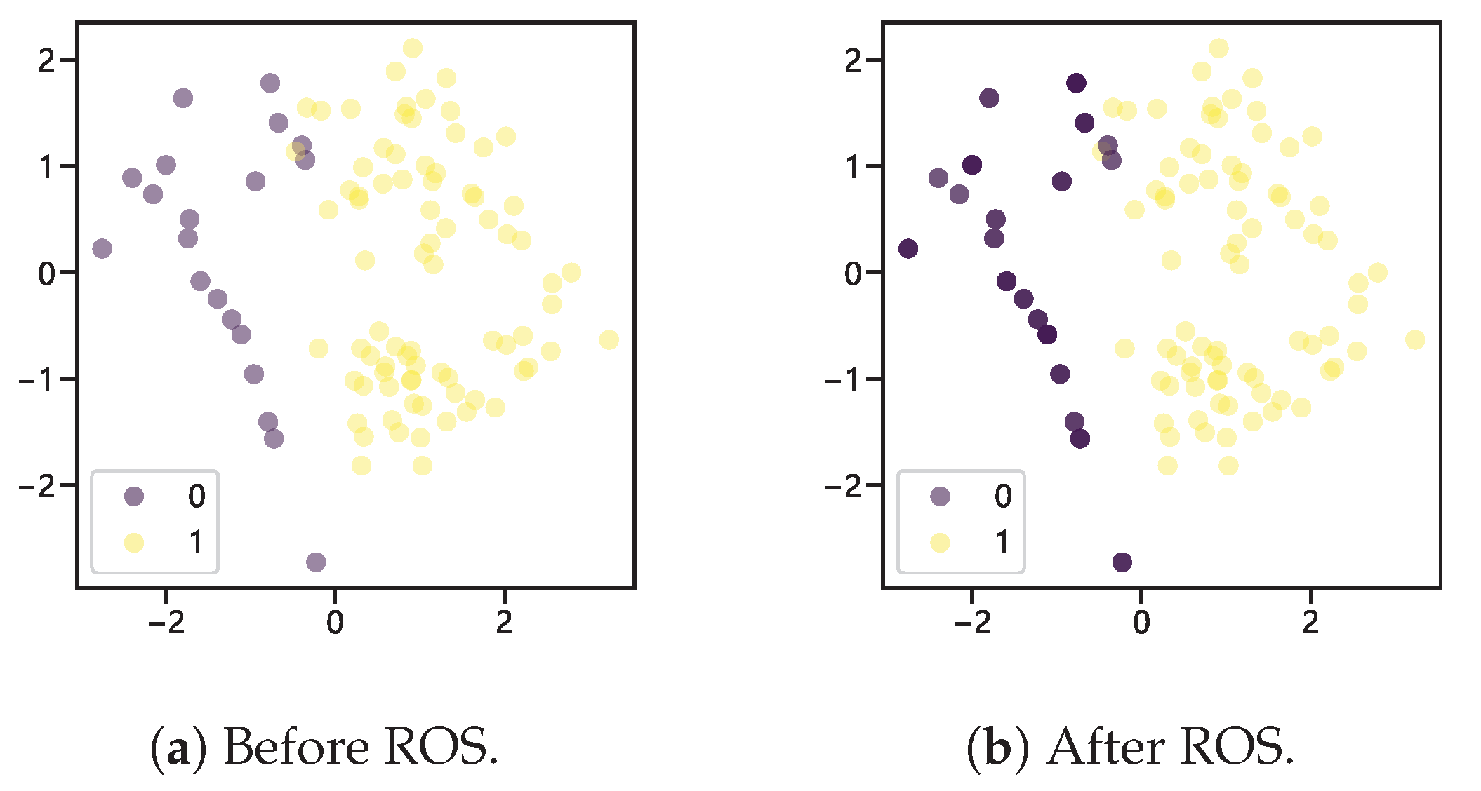
In ordinary random oversampling, when too many synthetic samples are introduced in the majority class samples, the main solution is to copy some random samples from the minority class, which does not add any new information and may render the classifier overfitted. As shown in Figure 1a, “0” and “1” represent the sample category labels, i.e., minority class and majority class, respectively. The repeated generation of samples causes the newly generated minority class samples to overlap with each other, and the color of the example sample points in Figure 1b deepens. To mitigate this problem, we generate random noise at each randomly generated sample point using a smoothed Bootstrap, i.e., sampling from the kernel density estimate of the data points [17]. Assuming that K is a symmetric kernel density function with a variance of 1, the standard kernel density estimate of f(x) is

$${\widehat{f}}_n\left(x\right)=\frac{1}{nh}\sum _{i=1}^{n}K\left(\frac{x-X_i}{h}\right)$$

where h is the smoothing parameter. The corresponding distribution function is as follows:

$${\widehat{F}}_n\left(x\right)={\int }_{(-\infty )}^X{\widehat{f}}_n\left(t\right)dt$$

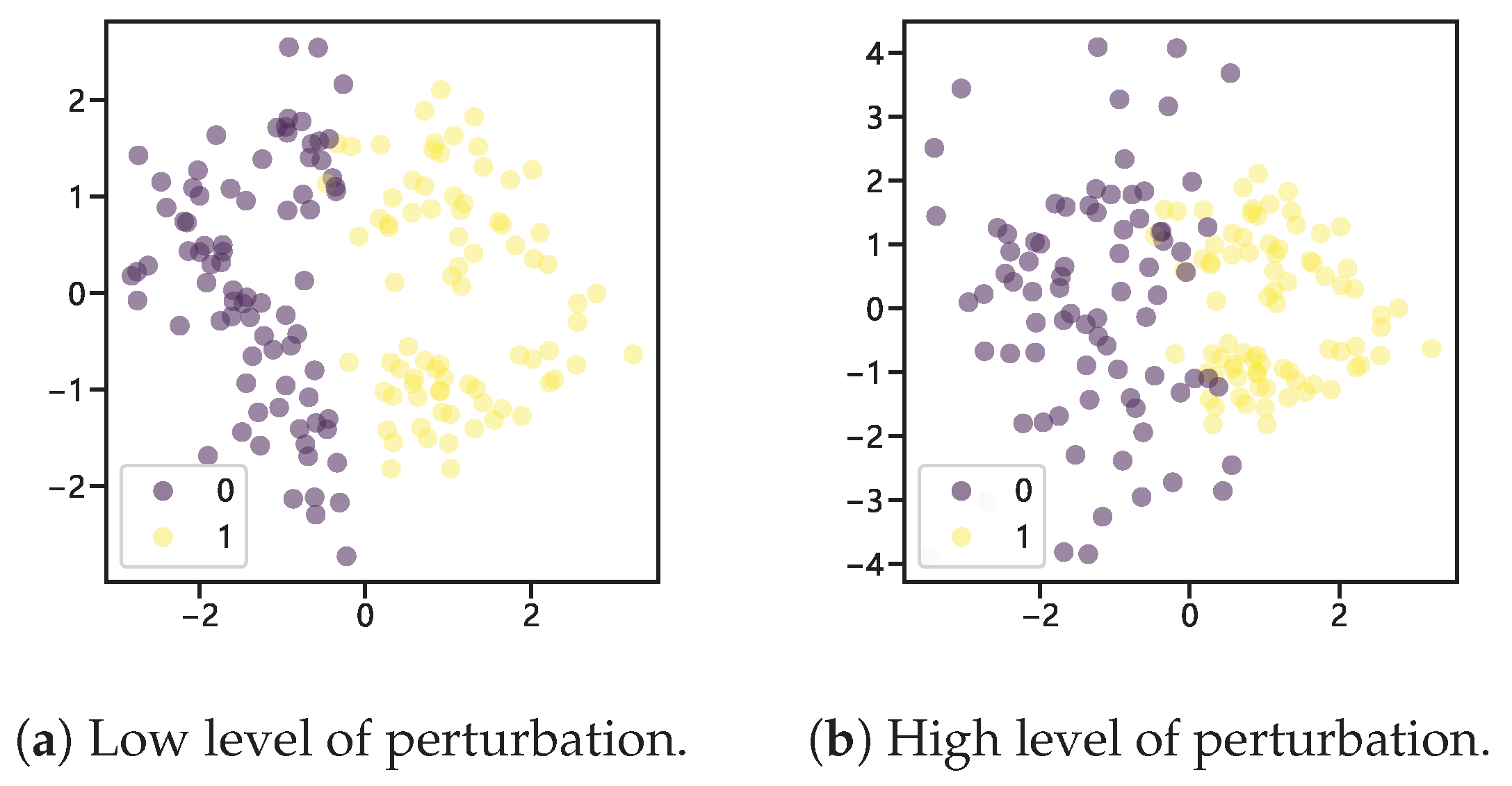
The sample points generated after adding a perturbation factor to the random oversampling process to allow for small perturbations in the randomly generated samples are shown in Figure 2, representing two degrees of perturbation. After the parameter has been perturbed by adding a small amount of noise, the randomly generated samples no longer overlap.

2.2. Step Two: Balanced Data Subset

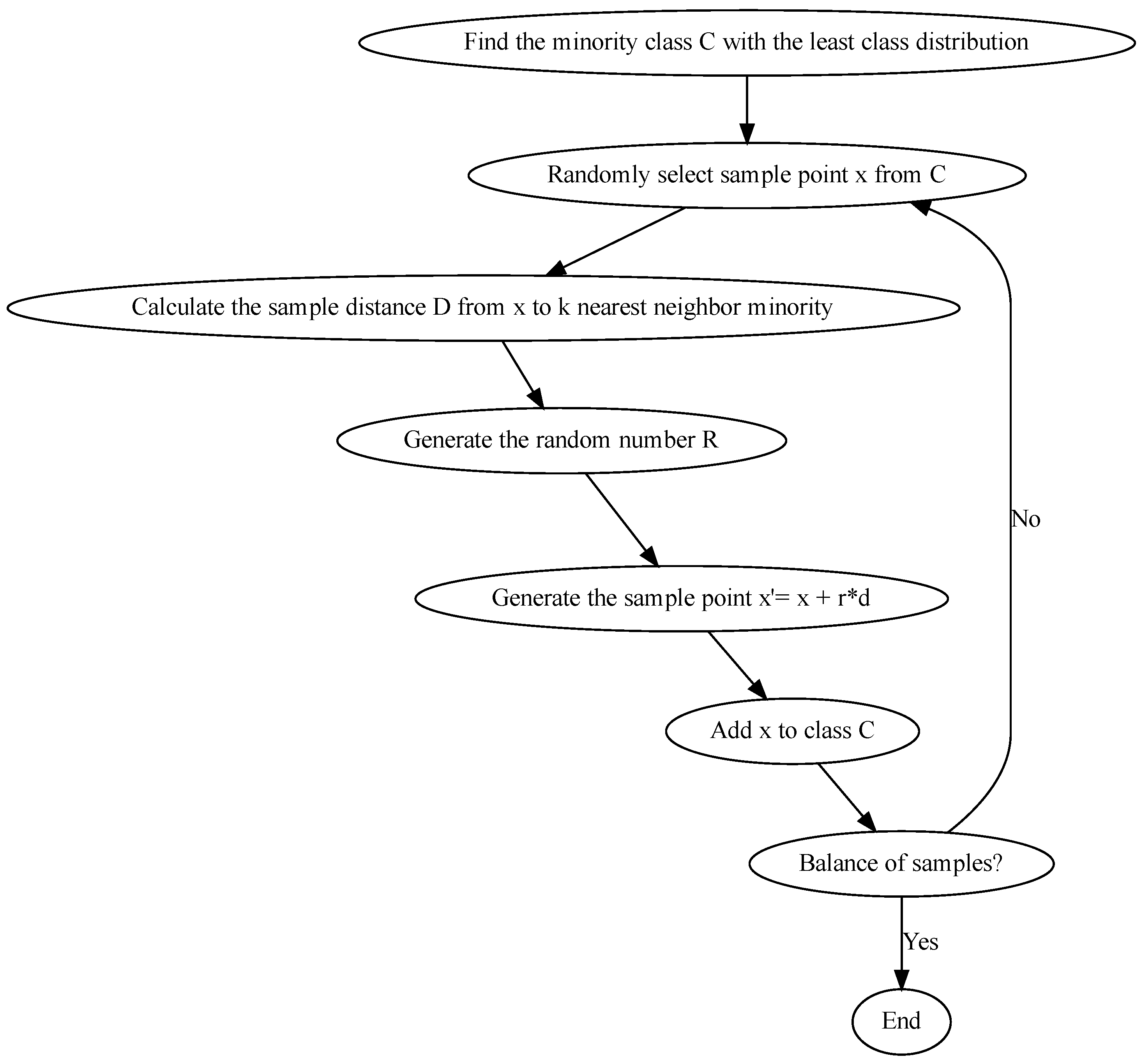
Because of its convenience and robustness in the sampling process, SMOTE is widely used to deal with imbalanced data. SMOTE has had a profound impact on supervised learning, unsupervised learning, and multi-class categorization, and it is an important benchmark with respect to algorithms for imbalanced data [18]. SMOTE creates interpolation between the samples of the minority class instances in the defined neighborhood via obtaining K-nearest neighbors of sample X in the minority class, randomly selecting one of the samples in the set of nearest neighbors, denoted as $X_i$, and the newly generated minority class samples are

$$X_{new}=X_{origin}+rand\times \left(X_i-X_{origin}\right),i=1,2,\dots ,n$$

where $rand$ is a randomly selected number in $(0,1)$ that generates minority class samples at a rate of approximately $\frac{1}{R}-1,R=\frac{positivesamples}{negativesamples}$. The process of SMOTE can be summarized as follows:

1

Find the minority class C with the lowest class distribution in the datasets.

2

Randomly select a data point x from $classC$, which is $x_{origin}$.

3

Calculate the distance d from point $x_{origin}$ to its K-nearest neighbors that belong to the minority class.

4

Randomly generate a number (rand) between [0, 1] and multiply it by distance d to generate a new sample point $x_{new}$ centered at $x_{origin}$. This process is performed based on the above formula.

5

Add $x_{new}$ to class C.

6

Repeat steps 2–5 until the number of samples in each class is balanced.

This process is summarized in Figure 3.

2.3. Step Three: Clear Boundary Noise

Random oversampling and SMOTE, with the addition of perturbation, ensure that sufficient minority class samples are generated, while undersampling the majority class corrects for the excess noise generated during both oversampling processes. Stage three involves the use of Tomek links, which can be defined as follows:

$$(x_i,x_j)\mathrm{denote}\mathrm{Tomek}\mathrm{Links}\iff y_i\ne y_j\forall x_k,d(x_i,x_k)\ge d(x_i,x_j)\forall x_k,d(x_j,x_k)\ge d(x_i,x_j)$$

Above, d represents the distance between two samples; $x_i,x_j$ are two samples of different categories; and $x_k$ is any third sample in the dataset.

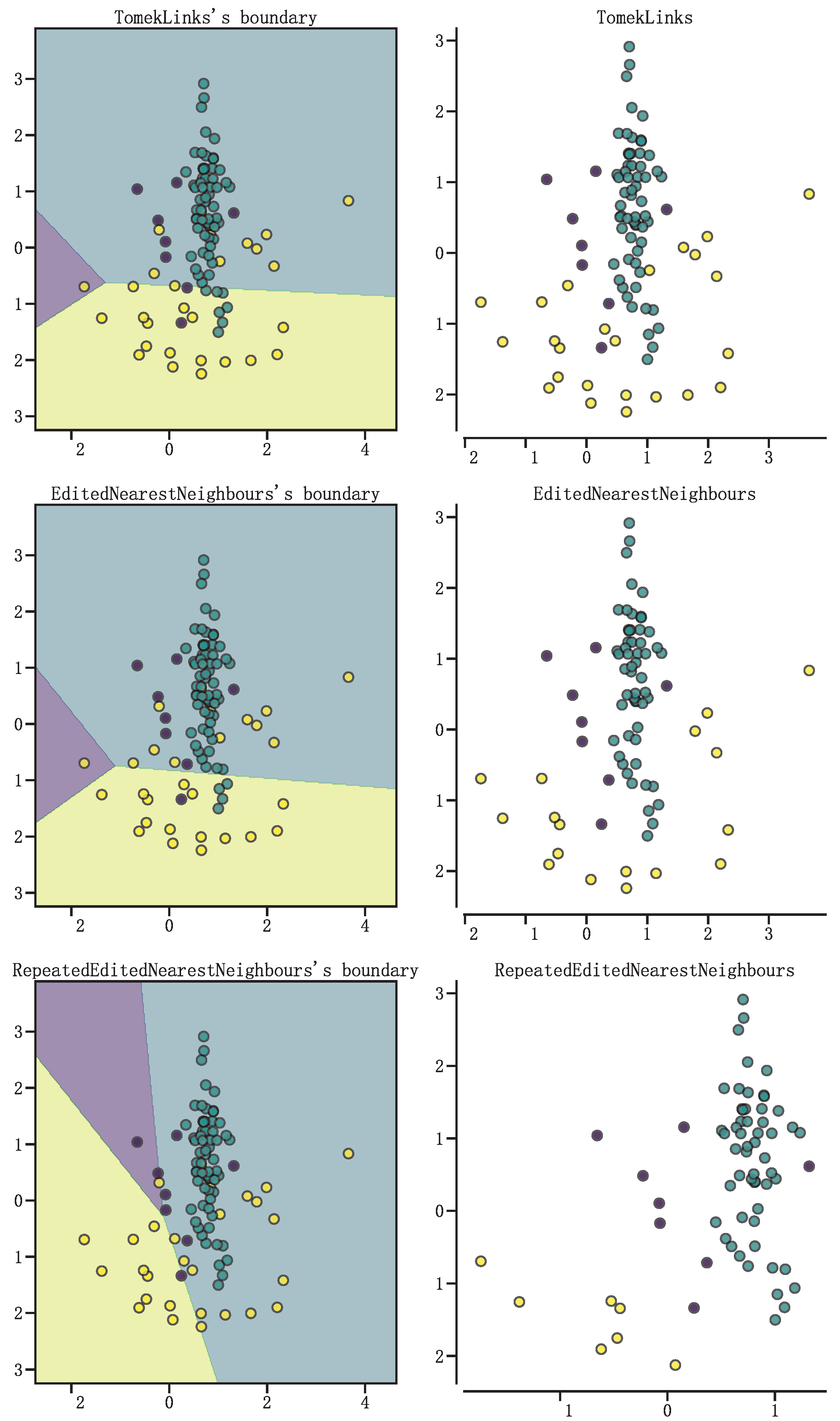
If the instance samples are labeled as Tomek links, then the pair of instance samples are either located near the classification boundary or are noisy instance samples. The characteristics of Tomek links allow for the deletion of samples that retain more sample points relative to those retained through other forms of deletion in undersampling. In Figure 4, three algorithms for selecting deleted sample points for undersampling are compared, and the undersampling algorithms used from top to bottom are Tomek links, ENN (edited nearest neighbors), and RENN (repeated edited nearest neighbors).

As can be seen in Figure 4, Tomek links have the shallowest degree of undersampling of the sample set compared to the two types of undersampling, ENN and RENN. In order to ensure the greatest sample size possible and remove useless samples, after random oversampling and SMOTE, we employ a Tomek links algorithm that uses dynamic temporal distance warping as a distance metric. Dynamic temporal warping (DTW) is an algorithm used to measure the similarity of two time series. DTW allows for a certain amount of deformation of a time series in the temporal dimension and is therefore more suitable than the traditional Euclidean distance for measuring the similarity of time series [12,19]. The algorithm for DTW is as follows:

1

Construct a matrix in which each element represents the distance between two time series at the corresponding position.

2

Start at the top left corner of the matrix and traverse the matrix along the diagonal to the bottom right corner.

3

At each position, select the distance at which d is minimized.

4

Repeat steps 2–3 until you reach the lower right corner of the matrix.

5

The element in the lower right corner of the matrix is the DTW distance between the two time series.

The TLDTW undersampling algorithm extended to time series data removes boundary noise from time series data to more efficiently create balanced classes. Like Tomek links, TLDTW also has the option of unilateral or bilateral undersampling, and bilateral TLDTW undersampling is used in SMOTE TLDTW.

Using SMOTE and TLDTW will output the data matrix $X_f$; the corresponding flow is shown in Algorithm 1. In the Experiments section, the three-stage sampling algorithm proposed in this paper is analyzed.

Algorithm 1 Undersampling after SMOTE algorithm

Require: X: Initialize dataset, K: number of nearest neighbors Ensure: $DT{W}_{matrix}$: Dynamic time warping distance matrix, $DTW$: Dynamic time warping distance        if $Min\le K$ then             Random Oversampling X 3:    end if        T: Minority class sample number        $Sample\left[\right]\left[\right]$: The original array of minority class samples 6:    $Synthetic\left[\right]\left[\right]$: Synthetic samples array        $numattrs=$ Number of attributes        for i = 1 to T do // Loop through all minority class samples 9:          Calculate i’s K nearest neighbors, add category tags to array $Nnarray$              Randomly select $nn$ from i’s K nearest neighbors              for $attr=1,2,\cdots ,numattrs$ do Calculate 12:              $dif=Sample\left[nnarray\right[nn\left]\right]\left[attr\right]-Sample\left[i\right]\left[attr\right]$                    $gap=rand$ between 0 and 1                    $Synthetic\left[new\right]\left[attr\right]=Sample\left[i\right]\left[attr\right]+gap\times dif$: Generate new samples 15:        end for         end for         $X_f=Synthetic$ 18:   if $y!=\mathrm{target}\mathrm{sample}$ then               Record the Tomek Links               Record the sample indices 21:   end if         Delete the samples with Tomek Links         Return $X_f$

Decomposing a multi-class classification problem into a binary classification problem is a common approach [20,21,22].

When dealing with multi-classified data, SMOTE TLDTW is consistent with the TLDTW algorithm in its decomposition approach, using OVR (one vs. rest) decomposition, where a few classes are randomly oversampled with respect to the set K value of SMOTE at each decomposition. To improve the generation of samples, SMOTE is then used to generate the sample size of the minority classes up to the number of the maximum number of classes in the datasets.

3. Experiments

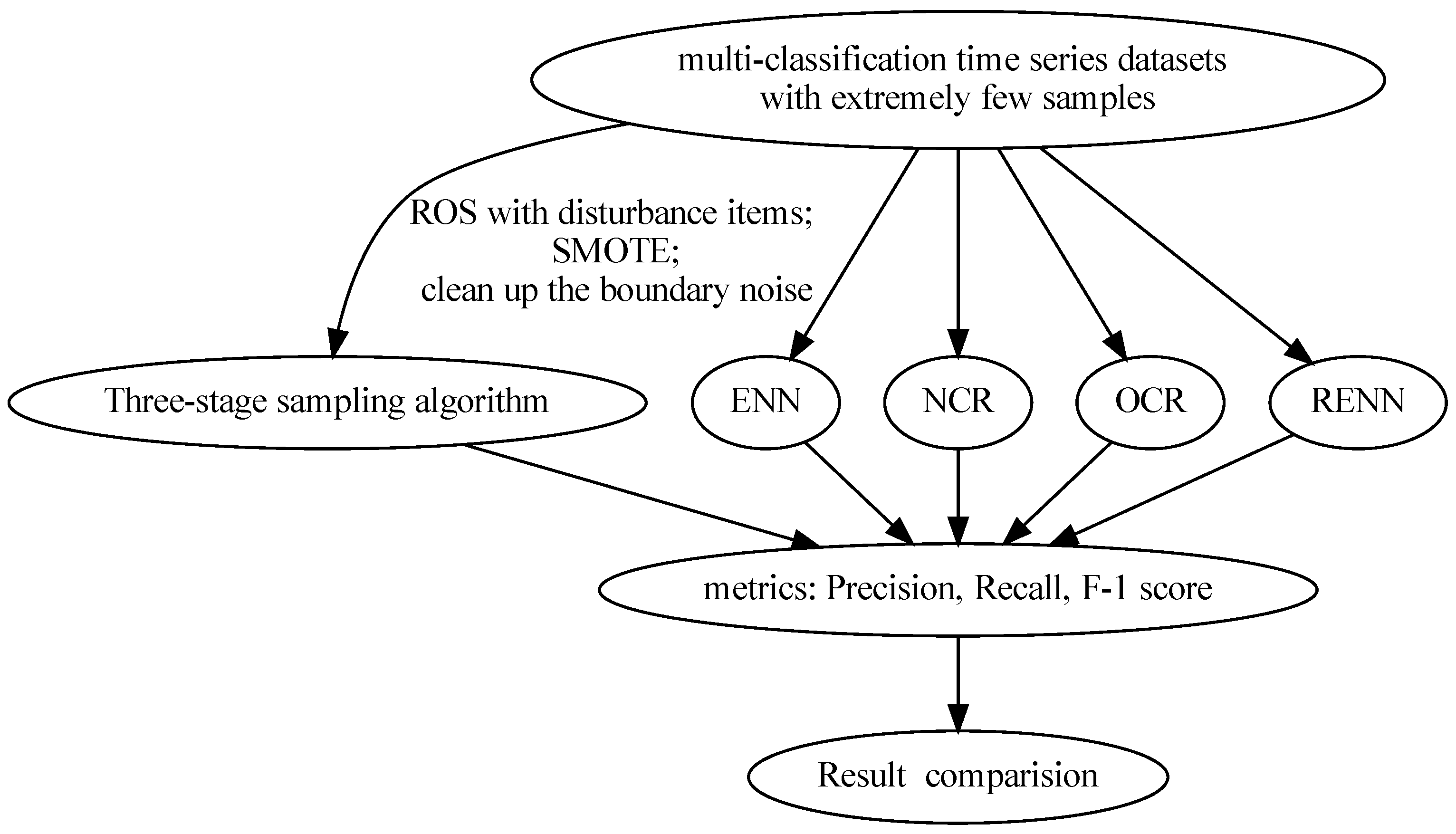
Throughout the Experiments section, this paper employs imbalanced time series datasets, some of which have extremely scarce minority class samples. The datasets used, evaluation metrics employed, and other benchmark algorithms used for comparison will be elaborated upon. The experimental procedure is illustrated in the following flowchart (Figure 5).

3.1. Data Description

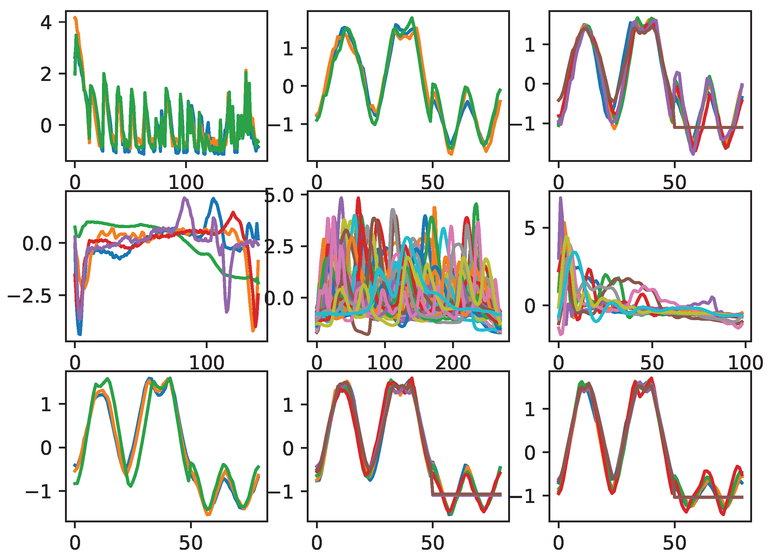
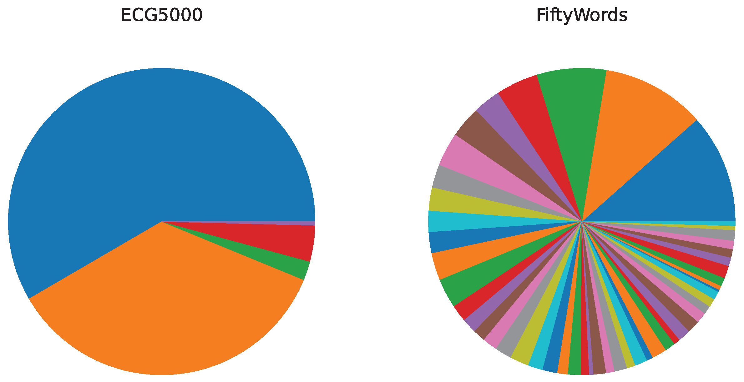
Nine datasets from the UCR dataset were used in this study, and their visualizations are shown in Figure 6 [23]. The horizontal axis in Figure 6 represents the sequence, and the vertical axis represents the values taken from the time series. The nine multicategorical datasets have different numbers of categories as well as disparate majority-to-minority ratios, and the degree of data imbalance in these multicategorical time series datasets ranges from slight to severe.

Table 1. The imbalanced rates of datasets.

Datasets	Imbalance Rate
ChlorineConcentration	2.88
DistalPhalanxOutlineAgeGroup	8.57
DistalPhalanxTW	11.83
ECG5000	146.00
FiftyWords	52.00
MedicalImages	33.83
MiddlePhalanxOutlineAgeGroup	4.31
MiddlePhalanxTW	6.40
ProximalPhalanxTW	11.25

shows the imbalance rate of the multicategorical imbalanced time series dataset. The imbalance rate (IR) was calculated using the number of samples of the maximum and minimum majority classes $IR=\frac{N_{maj}}{N_{min}}$, where $N_{maj}$ denotes the number of samples in the maximum majority class, and $N_{min}$ indicates the number of samples in the minimum minority class. This formula can reflect the degree of imbalance in the dataset. Of the nine datasets used for experiments in this study, FiftyWords has the largest number of sample classes, 49, and the smallest number of samples, only 1. In addition to FiftyWords, there are some minority classes in the ECG5000 dataset that have very few samples, with the smallest minority class having a sample size of two. Their data distributions are shown in Figure 7.

3.2. Metrics

In order to calculate precision, recall, and F1-score for multi-classification, the macro average precision, recall, and F1-score shown below were used correspondingly [24]:

$$Precision=\frac{TP}{TP+FP},$$

(1)

$$Recall=\frac{TP}{TP+FN},$$

(2)

$$F1-score=\frac{2\times Precision\times Recall}{Precision+Recall},$$

(3)

$$MacroPrecision=\frac{1}{N}\left(\sum _{i=1}^{N}Precisio{n}_{class=i}\right),$$

(4)

$$MacroRecall=\frac{1}{N}\left(\sum _{i=1}^{N}Recal{l}_{class=i}\right),$$

(5)

$$MacroF1-score=\frac{1}{N}\left(\sum _{i=1}^{N}F1-scor{e}_{class=i}\right).$$

(6)

3.3. Other Undersampling Algorithms, Classifiers, and Parameters

The four most representative undersampling algorithms, ENN, RENN, OSS, and NCR, were selected for comparison. OSS and NCR combine the ideas of selecting deleted samples and selecting retained samples. OSS selects retained samples through the CNN algorithm and deleted samples through Tomek links; NCR selects the retained samples through the CNN algorithm and deleted samples through the ENN; and NCR selects retained samples via the CNN algorithm and deleted samples via ENN. The undersampling algorithm selected in this paper is an algorithm in which undersampling is performed via selecting the deleted samples. In the three-stage sampling algorithm of this paper, TLDTW is the third step of SMOTE TLDTW, so TLDTW was also used to make comparisons.

The parameters were set according to the most stable and commonly used values for each type of algorithm. TLDTW uses one-sided undersampling, and only the majority class is censored. OSS uses the nearest neighbor of K = 1, K = 5 is set in SMOTE TLDTW, and the insufficient minority class samples are randomly oversampled up to the level of K = 5; then, SMOTE oversampling is performed, and the noisy data are cleaned using the two-sided TLDTW. The number of nearest neighbors of NCR is set to K = 3. The ROCKET (random convolutional kernel transform) classifier has a neural network structure but only one hyperparameter K. Compared to the other classifiers, the impact of this hyperparameter is relatively small; thus, it was chosen as the predictive model, with the parameter set to 500 [25].

4. Results and Discussion

Table 2. The performance of SMOTE TLDTW.

Datasets	Precision	Recall	F1-Score
ChlorineConcentration	0.6577	0.6633	0.6602
DistalPhalanxOutlineAgeGroup	0.6576	0.7178	0.6739
DistalPhalanxTW	0.4803	0.4622	0.4680
MedicalImages	0.7507	0.7397	0.7311
MiddlePhalanxOutlineAgeGroup	0.4351	0.4064	0.4070
MiddlePhalanxTW	0.4004	0.4052	0.4010
ProximalPhalanxTW	0.5583	0.5075	0.5170
ECG5000	0.6998	0.5904	0.6171
FiftyWords	0.7156	0.7261	0.6901

shows that the performance values of SMOTE TLDTW for the minority classes of imbalanced time series multiclassification datasets with very small sample sizes were all improved, with the highest precision, recall, and F1-score obtained for the MedicalImages dataset at 0.7507, 0.7397, and 0.7311, respectively.

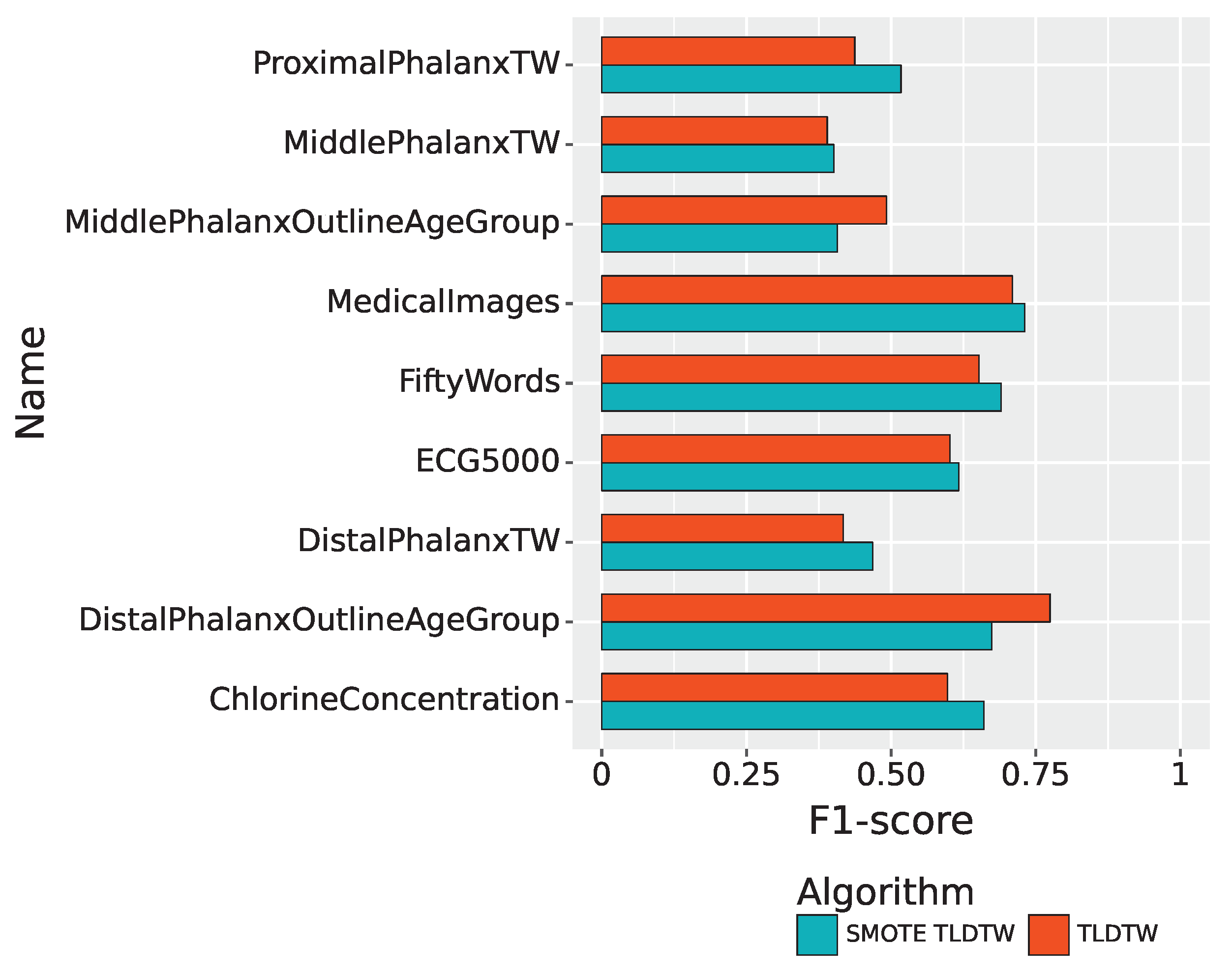
The F1-score of the two sampling algorithms, TLDTW and SMOTE TLDTW, for the imbalanced multiclassified time series datasets is shown in Figure 8. Regarding the nine imbalanced time series multiclassification datasets, TLDTW outperformed SMOTE TLDTW with respect to two datasets, namely, DistalPhalanxOutlineAgeGroup and MiddlePhalanxOutlineAgeGroup, with more samples from a few classes, yielding F1-scores of 0.7746 and 0.4922, respectively; SMOTE TLDTW had higher F1-score for the remaining seven datasets. It can be seen that TLDTW had better F1-score than SMOTE TLDTW for a few datasets with large sample sizes, but for a few datasets with severely insufficient sample sizes, such as ProximalPhalanxTW, ECG5000, and FiftyWords, which have only 16, 2, 1, and 6 samples, in a few categories, such as MedicalImages and other datasets, the F1-score of SMOTE TLDTW was better than that of TLDTW; these scores were 0.5170, 0.6171, 0.6901, and 0.7311 for the above datasets, respectively.

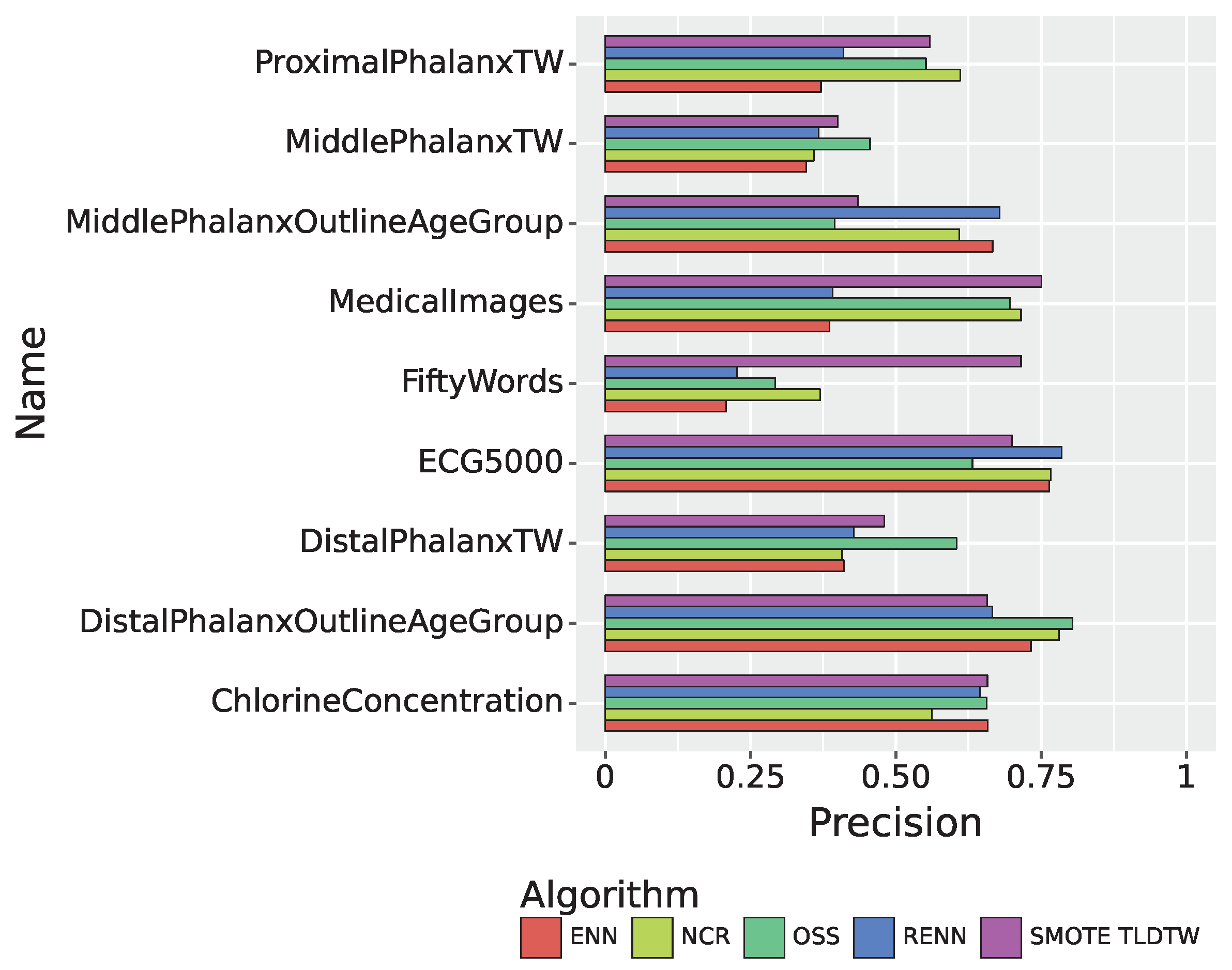
As shown in Figure 9, in the multiclassified datasets, the precision of SMOTE TLDTW in the FiftyWords dataset, which has many categories and a small number of minority classes, was much better than that of ENN, RENN, OSS, and NCR, with a precision of 0.7156.

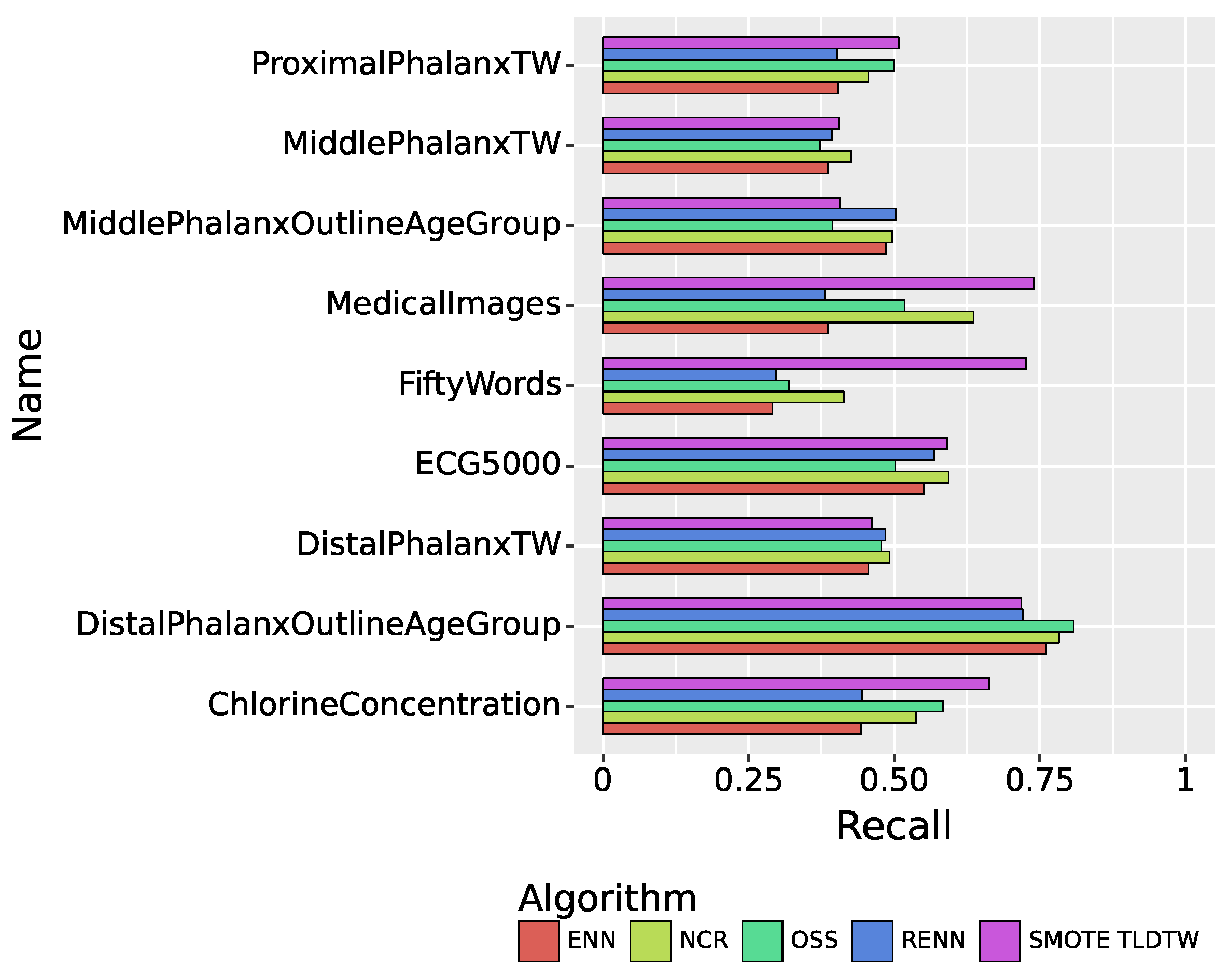
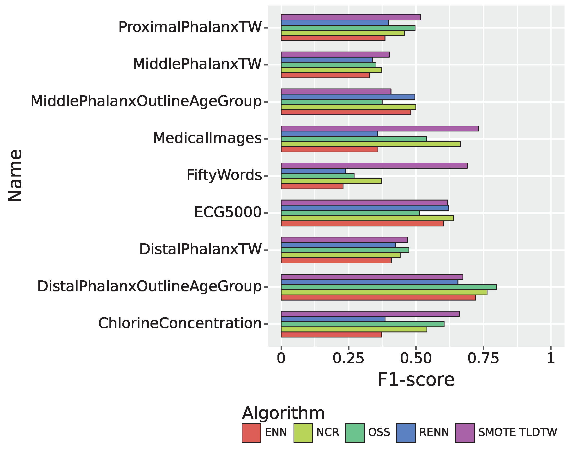
Figure 10 summarizes the recall performance of the five sampling algorithms. In the multiclassified dataset, SMOTE TLDTW still significantly outperformed the other four undersampling algorithms with respect to FiftyWords and MedicalImages, which have a large number of categories and a sparse minority of categories, respectively. The F1-score comparison results of the five sampling algorithms are shown in Figure 11, summarizing the results of the nine imbalanced time series datasets. SMOTE TLDTW outperformed the other four undersampling algorithms for five datasets, namely, MedicalImages, FiftyWords, ChlorineConcentration, ProximalPhalanxTW, and MiddlePhalanxTW. The F1-scores of the SMOTE TLDTW algorithm for these five datasets are 0.7311, 0.6901, 0.6602, 0.5170, and 0.4010, respectively. For the nine imbalanced time series multiclassified datasets, for the most categorized dataset FiftyWords, SMOTE TLDTW facilitated increases of 200.71%, 188.74%, 155.29%, and 85.61% relative to ENN, RENN, OSS, and NCR, respectively.

5. Conclusions

In this study, we proposed a three-stage sampling approach to alleviate the imbalance issue in multi-class time series data with extremely scarce minority samples. In the first stage, random oversampling with disturbances was performed to increase sample size. On this basis, in the second stage, SMOTE was employed to generate synthetic samples. The third stage involved the identification and removal of boundary noise, retaining clearer boundaries without losing too much information. The combination of these three stages provided an effective solution for these specific datasets. The experiments conducted on nine highly skewed datasets demonstrate that our three-stage approach achieves significant performance gains over other undersampling methods. For the FiftyWords dataset with the most categories and fewest minority samples, our method improved macro accuracy by 200.71% and F1-score by 155.29% compared to benchmark algorithms. The results highlight the synergistic effects of random oversampling, SMOTE synthesis, and boundary noise removal in tackling the imbalance problem. This three-stage sampling scheme provides a new direction for alleviating data scarcity and class imbalance in multi-class time series.

References

- Nespoli, A.; Niccolai, A.; Ogliari, E.; Perego, G.; Collino, E.; Ronzio, D. Machine Learning Techniques for Solar Irradiation Nowcasting: Cloud Type Classification Forecast through Satellite Data and Imagery. Appl. Energy 2022, 305, 117834. [Google Scholar] [CrossRef]
- Stefenon, S.F.; Singh, G.; Yow, K.C.; Cimatti, A. Semi-ProtoPNet Deep Neural Network for the Classification of Defective Power Grid Distribution Structures. Sensors 2022, 22, 4859. [Google Scholar] [CrossRef] [PubMed]
- He, H.; Ma, Y. (Eds.) Imbalanced Learning: Foundations, Algorithms, and Applications; John Wiley & Sons, Inc: Hoboken, NJ, USA, 2013. [Google Scholar]
- Thabtah, F.; Hammoud, S.; Kamalov, F.; Gonsalves, A. Data Imbalance in Classification: Experimental Evaluation. Inf. Sci. 2020, 513, 429–441. [Google Scholar] [CrossRef]
- Cao, L.; Zhai, Y. Imbalanced Data Classification Based on a Hybrid Resampling SVM Method. In Proceedings of the 2015 IEEE 12th Intl Conf on Ubiquitous Intelligence and Computing and 2015 IEEE 12th Intl Conf on Autonomic and Trusted Computing and 2015 IEEE 15th Intl Conf on Scalable Computing and Communications and Its Associated Workshops (UIC-ATC-ScalCom), Beijing, China, 10–14 August 2015; pp. 1533–1536. [Google Scholar] [CrossRef]
- Ganganwar, V. An Overview of Classification Algorithms for Imbalanced Datasets. Int. J. Emerg. Technol. Adv. Eng. 2012, 2, 42–47. [Google Scholar]
- Chawla, N.V.; Bowyer, K.W.; Hall, L.O.; Kegelmeyer, W.P. SMOTE: Synthetic Minority Over-sampling Technique. J. Artif. Intell. Res. 2002, 16, 321–357. [Google Scholar] [CrossRef]
- Han, H.; Wang, W.Y.; Mao, B.H. Borderline-SMOTE: A New Over-Sampling Method in Imbalanced Data Sets Learning. In Advances in Intelligent Computing, Proceedings of the International Conference on Intelligent Computing, ICIC 2005, Hefei, China, 23–26 August 2005; Lecture Notes in Computer Science; Huang, D.S., Zhang, X.P., Huang, G.B., Eds.; Springer: Berlin/Heidelberg, Germany, 2005; pp. 878–887. [Google Scholar] [CrossRef]
- Bunkhumpornpat, C.; Sinapiromsaran, K.; Lursinsap, C. DBSMOTE: Density-Based Synthetic Minority Over-sampling TEchnique. Appl. Intell. 2012, 36, 664–684. [Google Scholar] [CrossRef]
- Devi, D.; Biswas, S.K.; Purkayastha, B. A Review on Solution to Class Imbalance Problem: Undersampling Approaches. In Proceedings of the 2020 International Conference on Computational Performance Evaluation (ComPE), Shillong, India, 2–4 July 2020; pp. 626–631. [Google Scholar] [CrossRef]
- Wang, H.; Liu, X. Undersampling Bankruptcy Prediction: Taiwan Bankruptcy Data. PLoS ONE 2021, 16, e0254030. [Google Scholar] [CrossRef] [PubMed]
- Kubat, M.; Matwin, S. Addressing the Curse of Imbalanced Training Sets: One-Sided Selection. In Proceedings of the Fourteenth International Conference on Machine Learning, Nashville, TN, USA, 8–12 July 1997; Morgan Kaufmann: Burlington, MA, USA, 1997; pp. 179–186. [Google Scholar]
- Koziarski, M.; Woźniak, M.; Krawczyk, B. Combined Cleaning and Resampling Algorithm for Multi-Class Imbalanced Data with Label Noise. Knowl.-Based Syst. 2020, 204, 106223. [Google Scholar] [CrossRef]
- Kaur, H.; Pannu, H.S.; Malhi, A.K. A Systematic Review on Imbalanced Data Challenges in Machine Learning: Applications and Solutions. ACM Comput. Surv. 2019, 52, 79:1–79:36. [Google Scholar] [CrossRef]
- Aguiar, G.; Krawczyk, B.; Cano, A. A Survey on Learning from Imbalanced Data Streams: Taxonomy, Challenges, Empirical Study, and Reproducible Experimental Framework. Mach. Learn. 2023. [CrossRef]
- Zeng, M.; Zou, B.; Wei, F.; Liu, X.; Wang, L. Effective Prediction of Three Common Diseases by Combining SMOTE with Tomek Links Technique for Imbalanced Medical Data. In Proceedings of the 2016 IEEE International Conference of Online Analysis and Computing Science (ICOACS), Chongqing, China, 28–29 May 2016; pp. 225–228. [Google Scholar] [CrossRef]
- Wang, S. Optimizing the Smoothed Bootstrap. Ann. Inst. Stat. Math. 1995, 47, 65–80. [Google Scholar] [CrossRef]
- Fernandez, A.; Garcia, S.; Herrera, F.; Chawla, N.V. SMOTE for Learning from Imbalanced Data: Progress and Challenges, Marking the 15-Year Anniversary. J. Artif. Intell. Res. 2018, 61, 863–905. [Google Scholar] [CrossRef]
- Keogh, E.; Ratanamahatana, C.A. Exact Indexing of Dynamic Time Warping. Knowl. Inf. Syst. 2005, 7, 358–386. [Google Scholar] [CrossRef]
- Knerr, S.; Personnaz, L.; Dreyfus, G. Single-Layer Learning Revisited: A Stepwise Procedure for Building and Training a Neural Network. In Neurocomputing; Soulié, F.F., Hérault, J., Eds.; Springer: Berlin/Heidelberg, Germany, 1990; pp. 41–50. [Google Scholar] [CrossRef]
- Clark, P.; Boswell, R. Rule Induction with CN2: Some Recent Improvements. In Machine Learning—EWSL-91, Proceedings of the European Working Session on Learning, Porto, Portugal, 6–8 March 1991; Lecture Notes in Computer Science; Kodratoff, Y., Ed.; Springer: Berlin/Heidelberg, Germany, 1991; pp. 151–163. [Google Scholar] [CrossRef]
- Anand, R.; Mehrotra, K.; Mohan, C.; Ranka, S. Efficient Classification for Multiclass Problems Using Modular Neural Networks. IEEE Trans. Neural Netw. 1995, 6, 117–124. [Google Scholar] [CrossRef] [PubMed]
- Dau, H.A.; Bagnall, A.; Kamgar, K.; Yeh, C.C.M.; Zhu, Y.; Gharghabi, S.; Ratanamahatana, C.A.; Keogh, E. The UCR Time Series Archive. IEEE/CAA J. Autom. Sin. 2019, 6, 1293–1305. [Google Scholar] [CrossRef]
- Gowda, T.; You, W.; Lignos, C.; May, J. Macro-Average: Rare Types Are Important Too. In Proceedings of the 2021 Conference of the North American Chapter of the Association for Computational Linguistics: Human Language Technologies, Online, 6–11 June 2021; pp. 1138–1157. [Google Scholar] [CrossRef]
- Dempster, A.; Petitjean, F.; Webb, G.I. ROCKET: Exceptionally Fast and Accurate Time Series Classification Using Random Convolutional Kernels. Data Min. Knowl. Discov. 2020, 34, 1454–1495. [Google Scholar] [CrossRef]
Figure 1.
Comparison of before and after random oversampling.
Figure 2.
Two-degree perturbation of ROS.
Figure 3.
The SMOTE flowchart.
Figure 4.
Three undersampling algorithms.
Figure 5.
A research flow diagram including the data and the SMOTE TLDTW algorithm and other comparison groups with metrics.
Figure 6.
Visualization of multi-classification time series data.
Figure 7.
The distribution maps of ECG500 and FiftyWords.
Figure 8.
The F1-score of the SMOTE TLDTW and TLDTW.
Figure 9.
The precision of 9 imbalanced time series multiple-sample datasets.
Figure 10.
The recall of 9 imbalanced time-series multiclassified datasets.
Figure 11.
The F1-score of 9 imbalanced time-series multiclassified datasets.