Construction of Novel Bright-Dark Solitons and Breather Waves of Unstable Nonlinear Schrödinger Equations with Applications

Abstract

The unstable nonlinear Schrödinger equations (UNLSEs) are universal equations of the class of nonlinear integrable systems, which reveal the temporal changing of disruption in slightly stable and unstable media. In current paper, an improved auxiliary equation technique is proposed to obtain the wave results of UNLSE and modified UNLSE. Numerous varieties of results are generated in the mode of some special Jacobi elliptic functions and trigonometric and hyperbolic functions, many of which are distinctive and have significant applications such as pulse propagation in optical fibers. The exact soliton solutions also give information on the soliton interaction in unstable media. Furthermore, with the assistance of the suitable parameter values, various kinds of structures such as bright-dark, multi-wave structures, breather and kink-type solitons, and several periodic solitary waves are depicted that aid in the understanding of the physical interpretation of unstable nonlinear models. The various constructed solutions demonstrate the effectiveness of the suggested approach, which proves that the current technique may be applied to other nonlinear physical problems encountered in mathematical physics.

1. Introduction

The nonlinear Schrödinger equations (NLSEs) are fundamental nonlinear canonical evolution equations that are extensively used in several disciplines of both theoretical and applied sciences. The nonlinear equations are often employed in the modeling of many physical events, including the transmission line across optical fibers [1,2,3,4,5,6,7], attraction-repulsion chemotaxis models [8,9], the traveling of Langmuir waves in hot plasma [10], the propagation of rogue waves [11,12,13], depth water waves in oceans [14], ecology, and numerous others [15]. Partial differential equations (PDEs) are also derived for a population whose individuals randomly experience births, deaths, and size changes. PDEs are among the best mathematical tools for analyzing spatiotemporal processes. These nonlinear equations deal with non-linearity and dispersive effects at the same time and are one of the simplest forms of evolution equations. Due to their integrable characteristics, these nonlinear equations are widely used for the description of dynamics of localized stationary along with pulsating waves envelops. These nonlinear equations are known as universal equations because they explain how waves move through many physical systems. These equations are crucial tools for comprehending the physical analogies and variations in the nonlinear behaviour of dispersive waves. Rogue waves in nonlinear dispersive media are very thought provoking, for example, [16,17,18,19,20]. These rogue waves were initially examined in the background of water waves, and after that, they became an interesting topic for in-depth studies of nonlinear optics. The NLSEs are a basic part of the explanation of the construction of rogue waves that have been found in fiber optics [21,22], as well as in deep water [23,24,25,26].

With the achievements in the field of nonlinear science, many systematic and efficient methods have been formulated and improved for the finding of exact and approximate solutions of nonlinear evolution equations (NLEEs). These equations include the modified extended direct algebraic method [27], the modified simple equation method [28], the Jacobi elliptic function method [29,30], the modified extended mapping method [31], the semi-inverse variation method [32], the generalized Kudryashov method [33,34], the Bilinear residual network method [35], the modified extended tanh method [36], the sine-Gordon equation method [37], the tri-prong scheme [38], the Darboux transformation [39,40], the explicit spectral collection method [41], the generalized extended rational expansion method [42], the binary bell polynomials [43], the exponential fitting method [44], the auxiliary equation method [45], the improved auxiliary equation method [46], the modified F-expansion method [47], and many more [48,49].

The UNLSEs are NLSEs with space and time shuffled. Their role arises in plasma and elaborates the two-layer baroclinic instabilities [50,51]. In [50], the author showed that in the absence of dissipation of the equilibrated finite amplitude state causes oscillation, both of the mean flow and the baroclinic wave. The authors of [51] presented a nonlinear theory of the propagation of acoustic waves in piezoelectric semiconductors, based on an asymptotic expansion in multiple time and space scales. The UNLSE [51] has the following form:

$$i{U}_t+U_{xx}+2\nu {\left|U\right|}^{2}U-2\gamma U=0,$$

(1)

and the modified unstable nonlinear Schrödinger equation (mUNLSE) illustrates certain instabilities of modulated wave-trains [52], which have the following form:

$$i{U}_t+U_{xx}+2\nu {\left|U\right|}^{2}U-2\gamma U_{xt}=0,$$

(2)

where real valued arbitrary constants are $\gamma$ and $\nu$. These UNLSEs depict a temporal evolution of disruption in slightly stable or unstable media. Different methods are used to find exact wave solutions of unstable NLSE such as the modified extended mapping method [53], the $(G^{\prime }/G)$-expansion method [54], and many others. Researchers in [28] used the extended simple equation technique to construct the exact solutions of unstable NLSEs and to modify unstable NLSEs. The modified exponential rational function method was used by the researchers in [55] to obtain the traveling wave results of unstable NLSEs.

In this article, bright-dark solitons, breather-type waves, and other wave solutions of UNLSE and mUNLSE are achieved with the help of the suggested improved auxiliary equation technique. Several novel wave solutions of these models have been constructed by using the proposed technique in the form of the Jacobi elliptic function and trigonometric and hyperbolic functions, and many of them have important applications in mathematical physics. Additionally, plotted visuals are used to further explain the various innovative structures of the solutions that were found, including bright, dark, and kink-type solitons, and numerous periodic solitary waves. The main advantage of this method is that it provides solutions for different types of waves as well as the Jacobi elliptic function. Any nonlinear PDEs, including fractional-order nonlinear PDEs, can be solved using this method. The many successful findings demonstrate the effectiveness of the suggested method, demonstrating its applicability to various nonlinear dynamical models.

The rest of the paper is arranged as follows: In Section 2, the description of proposed method is given. The application of the suggested approach on UNLSE and mUNLSE is described in Section 3 and Section 4. The findings, discussion, and physical interpretation are covered thoroughly in Section 5. Finally, Section 6 presents the conclusion.

2. Proposed Improved Auxiliary Equation Method

In this section, a brief explanation of the improved auxiliary equation technique [46] for the construction of wave solutions of nonlinear evolution equations is stated. Consider a general nonlinear evolution equation in the following form as

$$G(U,U_x,U_t,U_{xt},U_{xx},U_{tt},\dots )=0,$$

(3)

where polynomial G contains $U(x,t)$ along with its partial derivatives $U_x$, $U_t$, $U_{xt}$, $U_{xx}$, $U_{tt}$ and so on.

Step 1: 

Consider the traveling wave transformation that converts $U(x,t)$ into $\Phi \left(\eta \right)$ as

$$U(x,t)=\Phi \left(\eta \right),\eta =\kappa x\pm \lambda t,$$

(4)

where Equation (4) has arbitrary constants $\kappa$ and $\lambda$. Using Equation (4) on Equation (3), it changes into an ordinary differential equation (ODE) as

$$H\left({\Phi }^{\prime },{\Phi }^{″},{\Phi }^{‴},\dots \right)=0,$$

(5)

where ${(}^{\prime })$ symbolizes the derivatives of $\Phi \left(\eta \right)$ with respect to $\eta$.

Step 2: 

Assume that Equation (5) has the following solution as

$$\Phi \left(\eta \right)=\sum _{i=0}^{2n}{c}_i{Z}^i\left(\eta \right),$$

(6)

where the arbitrary constants n have a positive integer value; this value can be determined with the help of the homogeneous balancing principle on Equation (5), and $Z\left(\eta \right)$ satisfies the new ansatz equation

$$Z^{\prime }\left(\eta \right)=\sqrt{a_0+a_{2}Z{\left(\eta \right)}^2+a_{4}Z{\left(\eta \right)}^4+a_{6}Z{\left(\eta \right)}^6},$$

(7)

where the constants $a_0,a_2,a_4,a_6$ are arbitrary. Assume that Equation (7) has solutions as

$$Z\left(\eta \right)=\frac{1}{2}\sqrt{-\frac{a_4}{a_6}(1\pm z\left(\eta \right))},$$

(8)

where $z\left(\eta \right)$ can be written in terms of Jacobi elliptic functions $sn(\eta ,m)$, $cn(\eta ,m)$, and $dn(\eta ,m)$. These Jacobi elliptic functions have m as its modulus; its value is $0<m<1$. As m achieves the value 0 or 1, the functions transform into trigonometric and hyperbolic functions.

Step 3: 

Use Equation (6) along with Equation (7) into Equation (5), collecting the coefficient of $Z^i\left(\eta \right)$ and setting equal to zero, it will give algebraic equations that have the parameters $a_0,a_2,a_4,a_6$, $c_i$, $\kappa$, and $\lambda$. These algebraic equations will be solved by software Mathematica, and the values of the parameters are obtained.

Step 4: 

Put the parameters along with Equation (8) into Equation (6), and the solution of Equation (3) is achieved.

3. Implementation of the Improved Auxiliary Equation Method on UNLSE

The UNLSE is a sort of NLSE with space and time shuffled. The role of this kind arises in plasma and elaborates the baroclinic instability of two layers and their lossless symmetrices [50,51]. As Equation (1) is complex, suppose the transformation in the following form as

$$U(x,t)=\Phi \left(\eta \right)e^{i\zeta },\eta =\kappa x+\lambda tand\zeta =\mu x+\sigma t,$$

(9)

where $\kappa$, $\lambda$, $\mu$, and $\sigma$ are the arbitrary constants. Applying the complex wave transformation Equation (9) on Equation (1) and separating into real and imaginary parts yields

$${\kappa }^2{\Phi }^{″}\left(\eta \right)-\left(2\gamma +{\mu }^2+\sigma \right)\Phi \left(\eta \right)+2\nu {\Phi }^3\left(\eta \right)=0,\mathrm{and}\lambda =-2k\mu .$$

(10)

Using the homogeneous balancing principal on Equation (10) gives the positive integer of value $n=1$. Assume the solution in the following form:

$$\Phi \left(\eta \right)=c_0+c_{1}Z\left(\eta \right)+c_{2}Z{\left(\eta \right)}^2.$$

(11)

Substituting Equation (11) along Equation (7) into Equation (10) yields a system of algebraic equations in parameters $a_0,a_2,a_4,a_6$, $c_0,c_1,c_2$, $\kappa$, $\lambda$, $\mu$, $\sigma$, $\gamma$ and $\nu$. By solving the system of algebraic equations with the help of Mathematica software, one obtains the values of parameters as

$$\begin{array}{cc}\hfill & \nu =\frac{\left(\sqrt{a_2^2-2a_0{a}_4}-a_2\right){\kappa }^2}{2c_0^2},\mu =\sqrt{a_2{\kappa }^2-2\gamma -\sigma +3{\kappa }^2\sqrt{a_2^2-2a_0{a}_4}},a_6=\frac{a_4\left(a_2-\sqrt{\left(a_2^2-2a_0{a}_4\right)}\right)}{4a_0},\hfill \\ \hfill & c_1=0,c_2=\frac{a_2{c}_0+\sqrt{a_2^2{c}_0^2-2a_0{a}_4{c}_0^2}}{a_0}.\hfill \end{array}$$

(12)

Using the parameters values of Equation (12) in Equation (8) generates

$$\begin{array}{c}\hfill Z\left(\eta \right)=c_0-\frac{(1\pm z\left(\eta \right))\left(a_2+\sqrt{a_2^2-2a_0{a}_4}\right)c_0}{a_2-\sqrt{a_2^2-2a_0{a}_4}}.\end{array}$$

(13)

By substituting the values $z\left(\eta \right)$ in the mode of the Jacobi elliptic functions, and by using Equation (11), the following cases are generated as

Case 1: 

If $a_0=\frac{a_4^3\left(m^2-1\right)}{32a_6^2{m}^2}$, $a_2=\frac{a_4^2\left(5m^2-1\right)}{16a_6{m}^2}$, $a_6>0$, then

$$\begin{array}{c}\hfill U_{11}\left(\eta \right)=(c_0-\frac{\left(a_2+\sqrt{a_2^2-2a_0{a}_4}\right)c_0(1\pm \mathrm{sn}\left(\tau \eta \right))}{a_2-\sqrt{a_2^2-2a_0{a}_4}})e^{i\zeta },\end{array}$$

(14)

or

$$\begin{array}{c}\hfill U_{12}\left(\eta \right)=(c_0-\frac{\left(a_2+\sqrt{a_2^2-2a_0{a}_4}\right)c_0\left(1\pm \frac{1}{m\mathrm{sn}\left(\tau \eta \right)}\right)}{a_2-\sqrt{a_2^2-2a_0{a}_4}})e^{i\zeta }.\end{array}$$

(15)

Substituting $m\to 1$, in Equation (15)

$$\begin{array}{c}\hfill U_{13}\left(\eta \right)=(c_0-\frac{\left(a_2+\sqrt{a_2^2-2a_0{a}_4}\right)c_0(1\pm coth\left(\tau \eta \right))}{a_2-\sqrt{a_2^2-2a_0{a}_4}})e^{i\zeta },\end{array}$$

(16)

where $\eta =\kappa (x-2\mu t)$ and $\zeta =(\sqrt{a_2{\kappa }^2-2\gamma -\sigma +3{\kappa }^2\sqrt{a_2^2-2a_0{a}_4}})x+\sigma t$.

Case 2: 

If $a_0=\frac{a_4^3\left(1-m^2\right)}{32a_6^2}$, $a_2=\frac{a_4^2\left(5-m^2\right)}{16a_6}$ and $a_6>0,$ then

$$\begin{array}{c}\hfill U_{21}\left(\eta \right)=(c_0-\frac{\left(a_2+\sqrt{a_2^2-2a_0{a}_4}\right)c_0(1\pm m\mathrm{sn}\left(\tau \eta \right))}{a_2-\sqrt{a_2^2-2a_0{a}_4}})e^{i\zeta },\end{array}$$

(17)

or

$$\begin{array}{c}\hfill U_{22}\left(\eta \right)=(c_0-\frac{\left(a_2+\sqrt{a_2^2-2a_0{a}_4}\right)c_0\left(1\pm \frac{1}{\mathrm{sn}\left(\tau \eta \right)}\right)}{a_2-\sqrt{a_2^2-2a_0{a}_4}})e^{i\zeta }.\end{array}$$

(18)

Substituting $m\to 1$, in Equation (17)

$$\begin{array}{c}\hfill U_{23}\left(\eta \right)=(c_0-\frac{\left(a_2+\sqrt{a_2^2-2a_0{a}_4}\right)c_0(1\pm tanh\left(\tau \eta \right))}{a_2-\sqrt{a_2^2-2a_0{a}_4}})e^{i\zeta },\end{array}$$

(19)

where $\eta =\kappa (x-2\mu t)$ and $\zeta =(\sqrt{a_2{\kappa }^2-2\gamma -\sigma +3{\kappa }^2\sqrt{a_2^2-2a_0{a}_4}})x+\sigma t$.

Case 3: 

If $a_0=\frac{a_4^3}{32a_6^2\left(1-m^2\right)}$, $a_2=\frac{a_4^2\left(4m^2-5\right)}{16a_6\left(m^2-1\right)}$, $a_6>0$, then

$$\begin{array}{c}\hfill U_{31}\left(\eta \right)=(c_0-\frac{\left(a_2+\sqrt{a_2^2-2a_0{a}_4}\right)c_0\left(1\pm \frac{1}{\mathrm{cn}\left(\tau \eta \right)}\right)}{a_2-\sqrt{a_2^2-2a_0{a}_4}})e^{i\zeta }.\end{array}$$

(20)

$$\begin{array}{c}\hfill U_{32}\left(\eta \right)=(c_0-\frac{\left(a_2+\sqrt{a_2^2-2a_0{a}_4}\right)c_0\left(1\pm \frac{\mathrm{dn}\left(\tau \eta \right)}{\sqrt{1-m^2}\mathrm{sn}\left(\tau \eta \right)}\right)}{a_2-\sqrt{a_2^2-2a_0{a}_4}})e^{i\zeta }.\end{array}$$

(21)

Substituting $m\to 0$ in Equation (21)

$$\begin{array}{c}\hfill U_{33}\left(\eta \right)=(c_0-\frac{\left(a_2+\sqrt{a_2^2-2a_0{a}_4}\right)c_0(1\pm csc\left(\tau \eta \right))}{a_2-\sqrt{a_2^2-2a_0{a}_4}})e^{i\zeta },\end{array}$$

(22)

where $\eta =\kappa (x-2\mu t)$ and $\zeta =(\sqrt{a_2{\kappa }^2-2\gamma -\sigma +3{\kappa }^2\sqrt{a_2^2-2a_0{a}_4}})x+\sigma t$.

The auxiliary Equation (7) has some special solutions, which are

Case 4: 

If $a_0=\frac{a_2^2\left(m^2-1\right)m^2}{a_4\left(2m^2-1\right)}$, $a_6=0$, $a_4<0$, $a_2\left(2m^2-1\right)>0$, then the parameters values are as follows:

$$\begin{array}{c}\hfill a_2=\frac{2\gamma +{\mu }^2+\sigma }{{\kappa }^2},a_4=-\frac{c_1^2\nu }{{\kappa }^2},c_0=0,c_2=0.\end{array}$$

(23)

Using the parameters values in Equation (23) generates

$$\begin{array}{c}\hfill U_{41}\left(\eta \right)=\sqrt{-\frac{m^2\left(2\gamma +{\mu }^2+\sigma \right)}{\left(2m^2-1\right)\nu }}\mathrm{cn}\left(\eta \sqrt{\frac{2\gamma +{\mu }^2+\sigma }{{\kappa }^2\left(2m^2-1\right)}}\right).\end{array}$$

(24)

Case 5: 

If $a_0=0,a_6=0$ and $a_2>0,a_4<0$, then the parameter values are as follows

$$\begin{array}{c}\hfill \sigma =a_2{\kappa }^2-2\gamma -{\mu }^2,a_4=-\frac{c_1^2\nu }{{\kappa }^2},c_0=c_2=0.\end{array}$$

(25)

Using the parameter values in Equation (25) generates

$$\begin{array}{c}\hfill U_{51}\left(\eta \right)=\sqrt{\frac{2\gamma +{\mu }^2+\sigma }{\nu }}\sec \mathrm{h}\left(\eta \sqrt{\frac{2\gamma +{\mu }^2+\sigma }{{\kappa }^2}}\right)e^{i\zeta }.\end{array}$$

(26)

Case 6: 

If $a_0=\frac{a_2^2}{4a_4},a_6=0$, and $a_2>0,a_4>0$, then the following parameters values are solved:

$$\begin{array}{c}\hfill a_2=\frac{2\gamma +{\mu }^2+\sigma }{{\kappa }^2},c_0=0,c_1=\pm \frac{i\sqrt{a_4}\kappa }{\sqrt{\nu }},c_2=0.\end{array}$$

(27)

Using parameters values Equation (27) generates

$$\begin{array}{c}\hfill U_{61}\left(\eta \right)=\pm \frac{i\sqrt{2\gamma +{\mu }^2+\sigma }}{\sqrt{2\nu }}tan\left(\eta \sqrt{\frac{2\gamma +{\mu }^2+\sigma }{2{\kappa }^2}}\right)e^{i\zeta }.\end{array}$$

(28)

4. Implementation of the Improved Auxiliary Equation Method on mUNLSE

The mUNLSE describes certain instabilities of modulated wave-trains and depicts a temporal evolution of disruption in slightly stable or unstable media [52]. As Equation (2) is also complex, suppose that the traveling wave transformation has the following form:

$$U(x,t)=\Psi \left(\eta \right)e^{i\zeta },\eta =\kappa x+\lambda t\mathrm{and}\zeta =\rho x+\omega t,$$

(29)

where arbitrary constants in the above equation are $\kappa ,\rho ,\lambda$, and $\omega$ real. Applying the complex wave transformation Equation (29) on Equation (2) and separating it into real and imaginary parts yields

$$\kappa (\kappa -\gamma \lambda ){\Psi }^{″}\left(\eta \right)+\left(\gamma \rho \omega -{\rho }^2-\omega \right)\Psi \left(\eta \right)+2\nu {\Psi }^3\left(\eta \right)=0,\lambda =\frac{\kappa (\gamma \omega -2\rho )}{1-\rho \gamma }.$$

(30)

Using the homogeneous balancing principal on Equation (30) gives a positive integer of the value $n=1$. Assume the solution in the following form:

$$\Psi \left(\eta \right)=c_0+c_{1}Z\left(\eta \right)+c_{2}Z{\left(\eta \right)}^2.$$

(31)

Substituting Equation (31) along Equation (7) into Equation (30) yields a system of algebraic in parameters $a_0,a_2,a_4,a_6$, $c_0,c_1,c_2$, $\kappa$, $\lambda$, $\rho$, $\omega$, $\gamma$, and $\nu$. On solving the system of algebraic equations with the aid of Mathematica software, the values of parameters are obtained as

$$\begin{array}{cc}\hfill & \nu =\frac{2a_4^2\kappa (\kappa -\gamma \lambda )}{\left(\sqrt{a_2^2-2a_0{a}_4}-a_2\right)c_2^2},\rho =\frac{\sqrt{\left(4a_2\kappa (\kappa -\gamma \lambda )+\omega \left({\gamma }^2\omega -4\right)\right)+12\sqrt{a_2^2-2a_0{a}_4}\kappa (\kappa -\gamma \lambda )}+\gamma \omega }{2},\hfill \\ & a_6=\frac{a_4^2}{2\left(a_2-\sqrt{a_2^2-2a_0{a}_4}\right)},c_0=\frac{\left(a_2+\sqrt{a_2^2-2a_0{a}_4}\right)c_2}{2a_4},c_1=0.\hfill \end{array}$$

(32)

Using the parameter values of Equation (32) in Equation (8) generates

$$\begin{array}{c}\hfill Z\left(\eta \right)=\frac{\sqrt{-\frac{\left(a_2-\sqrt{a_2^2-2a_0{a}_4}\right)(1\pm z\left(\eta \right))}{a_4}}}{\sqrt{2}}.\end{array}$$

(33)

By substituting the values $z\left(\eta \right)$ in the mode of Jacobi elliptic functions, and by using Equation (31), the following cases are generated as

Case 1: 

If $a_0=\frac{a_4^3\left(m^2-1\right)}{32a_6^2{m}^2}$, $a_2=\frac{a_4^2\left(5m^2-1\right)}{16a_6{m}^2}$, $a_6>0$, then

$$\begin{array}{c}\hfill U_{11}\left(\eta \right)=\frac{\pm \mathrm{sn}\left(\tau \eta \right)\left(\sqrt{a_2^2-2a_0{a}_4}-a_2\right)c_2}{2a_4}{e}^{i\zeta },\end{array}$$

(34)

or

$$\begin{array}{c}\hfill U_{12}\left(\eta \right)=\frac{\pm \frac{1}{m\mathrm{sn}\left(\tau \eta \right)}\left(\sqrt{a_2^2-2a_0{a}_4}-a_2\right)c_2}{2a_4}{e}^{i\zeta }.\end{array}$$

(35)

Substituting $m\to 1$ in Equation (35), we obtain

$$\begin{array}{c}\hfill U_{13}\left(\eta \right)=\frac{\pm coth\left(\tau \eta \right)\left(\sqrt{a_2^2-2a_0{a}_4}-a_2\right)c_2}{2a_4}{e}^{i\zeta },\end{array}$$

(36)

where $\eta =\kappa \left(x+\frac{(\gamma \omega -2\rho )}{1-\rho \gamma }t\right)$ and $\zeta =\frac{\sqrt{\left(4a_2\kappa (\kappa -\gamma \lambda )+\omega \left({\gamma }^2\omega -4\right)\right)+12\sqrt{a_2^2-2a_0{a}_4}\kappa (\kappa -\gamma \lambda )}+\gamma \omega }{2}x+\omega t$.

Case 2: 

If $a_0=\frac{a_4^3\left(1-m^2\right)}{32a_6^2}$, $a_2=\frac{a_4^2\left(5-m^2\right)}{16a_6}$ and $a_6>0,$ then

$$\begin{array}{c}\hfill U_{21}\left(\eta \right)=\frac{\pm \left(m\mathrm{sn}\left(\tau \eta \right)\right)\left(\sqrt{a_2^2-2a_0{a}_4}-a_2\right)c_2}{2a_4}{e}^{i\zeta },\end{array}$$

(37)

or

$$\begin{array}{c}\hfill U_{22}\left(\eta \right)=\frac{\pm \frac{1}{\mathrm{sn}\left(\tau \eta \right)}\left(\sqrt{a_2^2-2a_0{a}_4}-a_2\right)c_2}{2a_4}{e}^{i\zeta }.\end{array}$$

(38)

Substituting $m\to 1$ in Equation (37), we obtain

$$\begin{array}{c}\hfill U_{23}\left(\eta \right)=\frac{\pm tanh\left(\tau \eta \right)\left(\sqrt{a_2^2-2a_0{a}_4}-a_2\right)c_2}{2a_4}{e}^{i\zeta },\end{array}$$

(39)

where $\eta =\kappa \left(x+\frac{(\gamma \omega -2\rho )}{1-\rho \gamma }t\right)$ and $\zeta =\frac{\sqrt{\left(4a_2\kappa (\kappa -\gamma \lambda )+\omega \left({\gamma }^2\omega -4\right)\right)+12\sqrt{a_2^2-2a_0{a}_4}\kappa (\kappa -\gamma \lambda )}+\gamma \omega }{2}x+\omega t$.

Case 3: 

If $a_0=\frac{a_4^3}{32a_6^2\left(1-m^2\right)}$, $a_2=\frac{a_4^2\left(4m^2-5\right)}{16a_6\left(m^2-1\right)}$, $a_6>0$, then

$$\begin{array}{c}\hfill U_{31}\left(\eta \right)=\frac{\pm \frac{1}{\mathrm{cn}\left(\tau \eta \right)}\left(\sqrt{a_2^2-2a_0{a}_4}-a_2\right)c_2}{2a_4}{e}^{i\zeta },\end{array}$$

(40)

or

$$\begin{array}{c}\hfill U_{32}\left(\eta \right)=\frac{\pm \frac{\mathrm{dn}\left(\tau \eta \right)}{\sqrt{1-m^2}\mathrm{sn}\left(\tau \eta \right)}\left(\sqrt{a_2^2-2a_0{a}_4}-a_2\right)c_2}{2a_4}{e}^{i\zeta }.\end{array}$$

(41)

Substituting $m\to 0$ in Equation (41), we obtain

$$\begin{array}{c}\hfill U_{33}\left(\eta \right)=\frac{\pm csc\left(\tau \eta \right)\left(\sqrt{a_2^2-2a_0{a}_4}-a_2\right)c_2}{2a_4}{e}^{i\zeta },\end{array}$$

(42)

where $\eta =\kappa \left(x+\frac{(\gamma \omega -2\rho )}{1-\rho \gamma }t\right)$ and $\zeta =\frac{\sqrt{\left(4a_2\kappa (\kappa -\gamma \lambda )+\omega \left({\gamma }^2\omega -4\right)\right)+12\sqrt{a_2^2-2a_0{a}_4}\kappa (\kappa -\gamma \lambda )}+\gamma \omega }{2}x+\omega t$.

The auxiliary Equation (7) has some special solutions, which are as

Case 4: 

If $a_0=\frac{a_2^2\left(m^2-1\right)m^2}{a_4\left(2m^2-1\right)}$, $a_6=0$, $a_4<0$, $a_2\left(2m^2-1\right)>0$ then the parameters values are as follows:

$$\begin{array}{c}\hfill \rho =\frac{1}{\gamma },a_2=\frac{1}{{\gamma }^2\kappa (\kappa -\gamma \lambda )},a_4=-\frac{c_1^2\nu }{\kappa (\kappa -\gamma \lambda )},c_0=0,c_2=0.\end{array}$$

(43)

Using the parameter values in Equation (43) generates

$$\begin{array}{c}\hfill U_{41}\left(\eta \right)=\sqrt{-\frac{m^2}{{\gamma }^2\left(2m^2-1\right)\nu }}\mathrm{cn}\left(\eta \sqrt{\frac{1}{{\gamma }^2\kappa \left(2m^2-1\right)(\kappa -\gamma \lambda )}}\right).\end{array}$$

(44)

Case 5: 

If $a_0=0,a_6=0$, and $a_2>0,a_4<0$, then the parameter values are as follows:

$$\begin{array}{c}\hfill \omega =\frac{a_2\gamma \kappa \lambda -a_2{\kappa }^2+{\rho }^2}{\gamma \rho -1},a_4=-\frac{c_1^2\nu }{\kappa (\kappa -\gamma \lambda )},c_0=0,c_2=0.\end{array}$$

(45)

Using the parameter values in Equation (45) generates

$$\begin{array}{c}\hfill U_{51}\left(\eta \right)=\sqrt{\frac{a_2\kappa (\kappa -\gamma \lambda )}{\nu }}\sec \mathrm{h}\left(\sqrt{a_2}\eta \right)e^{i\zeta }.\end{array}$$

(46)

Case 6: 

If $a_0=\frac{a_2^2}{4a_4},a_6=0$ and $a_2>0,a_4>0$, then the parameters values are as follows

$$\begin{array}{c}\hfill \rho =\frac{1}{\gamma },a_2=\frac{1}{{\gamma }^2\kappa (\kappa -\gamma \lambda )},c_0=0,c_1=\pm \frac{i\sqrt{a_4}\sqrt{\kappa }\sqrt{\kappa -\gamma \lambda }}{\sqrt{\nu }},c_2=0.\end{array}$$

(47)

Using parameters values in Equation (47) generates

$$\begin{array}{c}\hfill U_{61}\left(\eta \right)=\frac{\pm i\sqrt{\frac{1}{\nu {\gamma }^2}}tan\left(\eta \sqrt{\frac{1}{2\left({\gamma }^2\kappa (\kappa -\gamma \lambda )\right)}}\right)}{\sqrt{2}}{e}^{i\zeta }.\end{array}$$

(48)

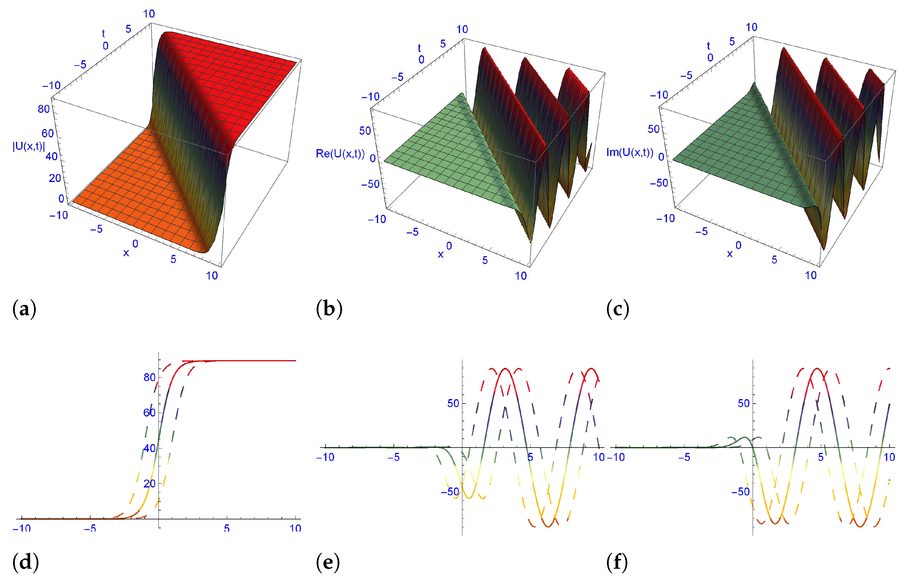
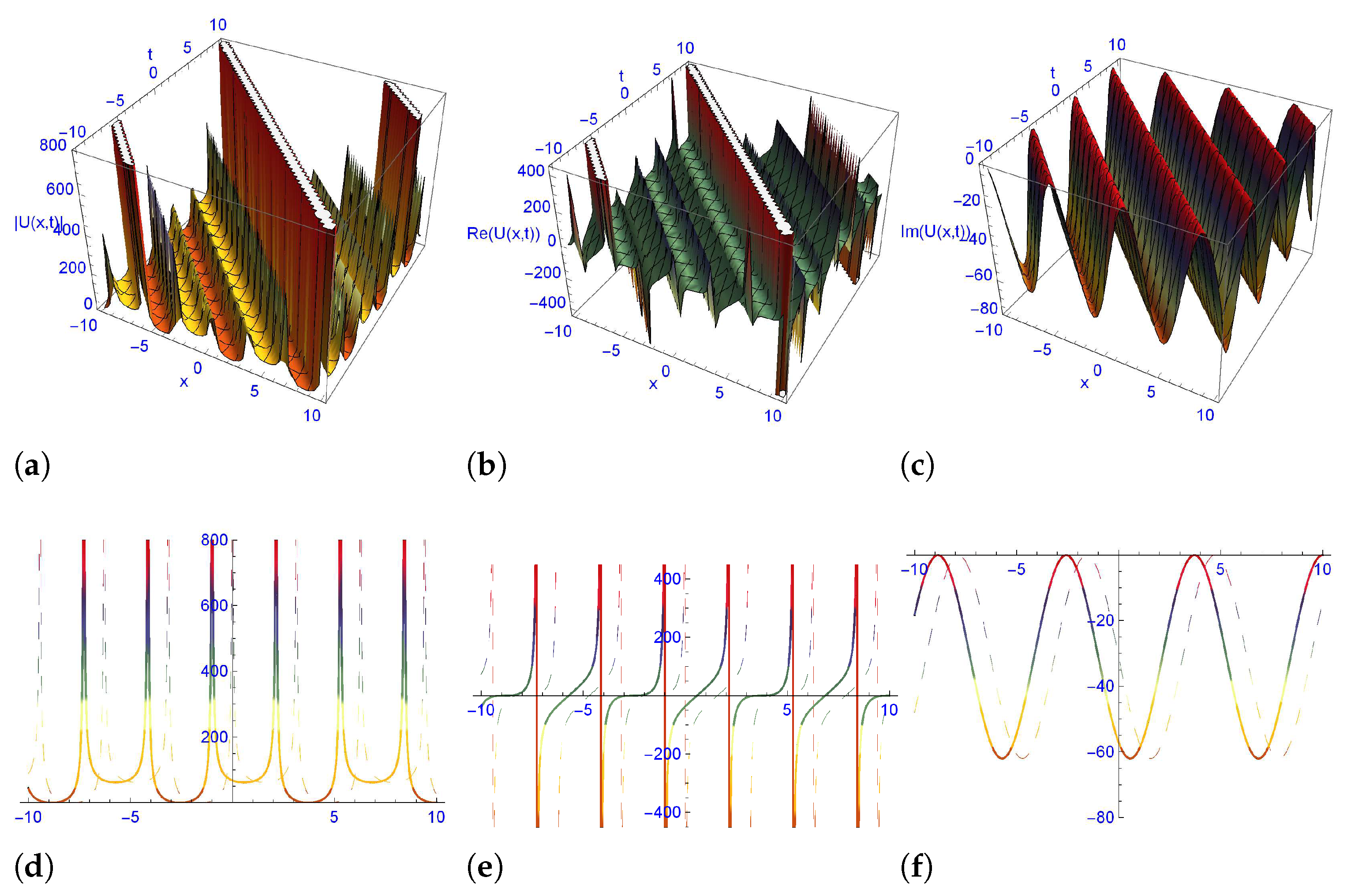
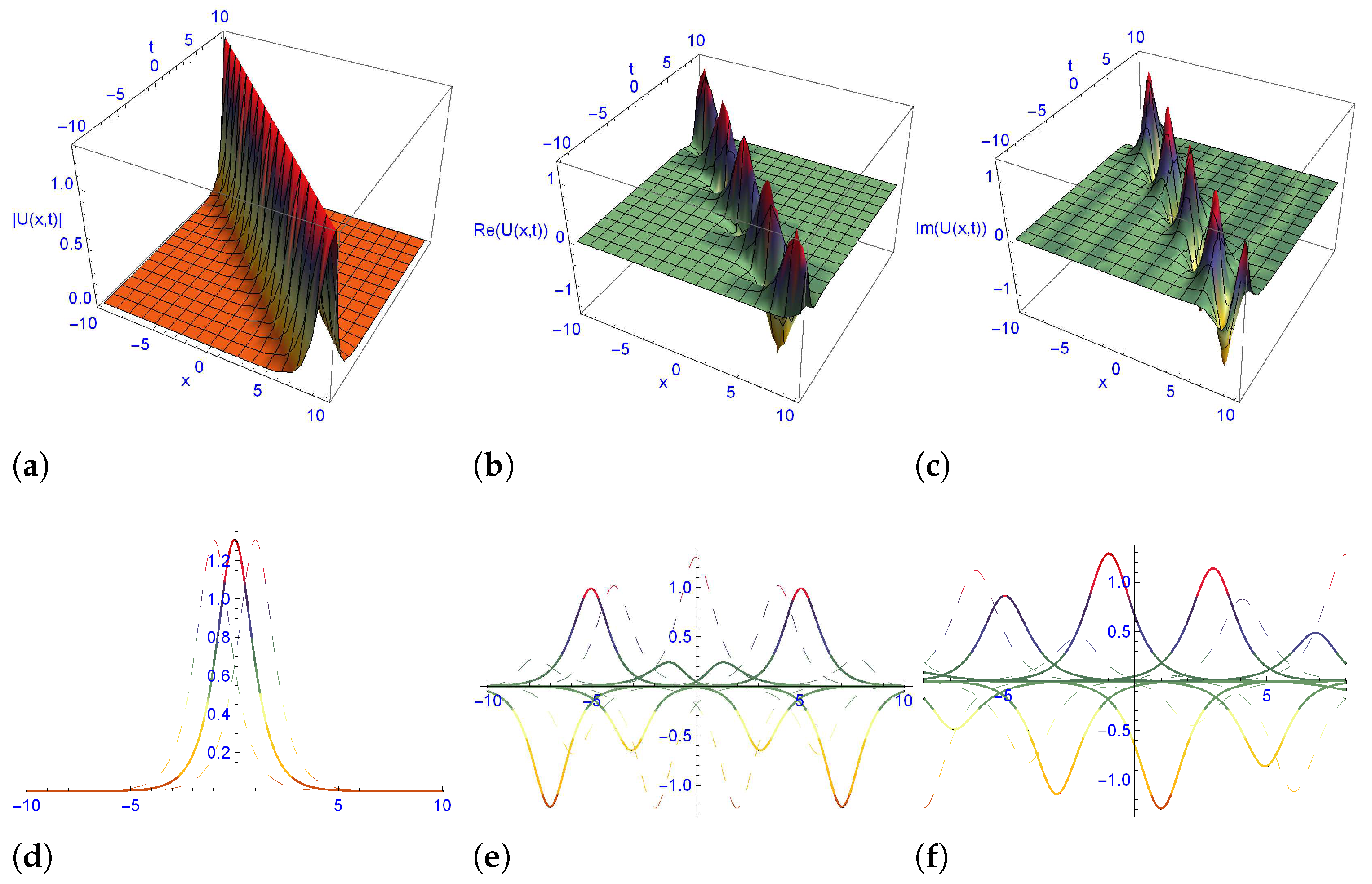
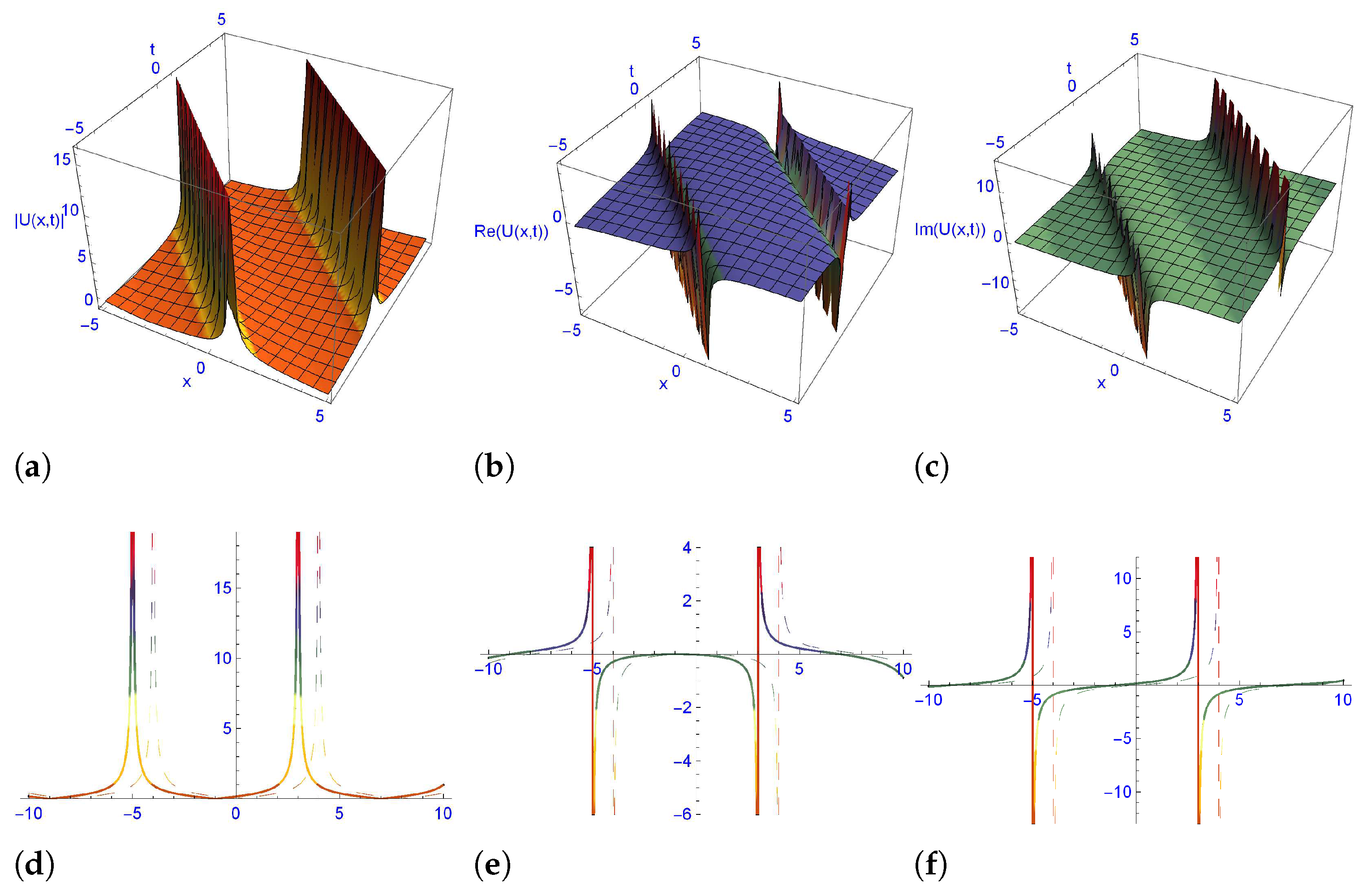
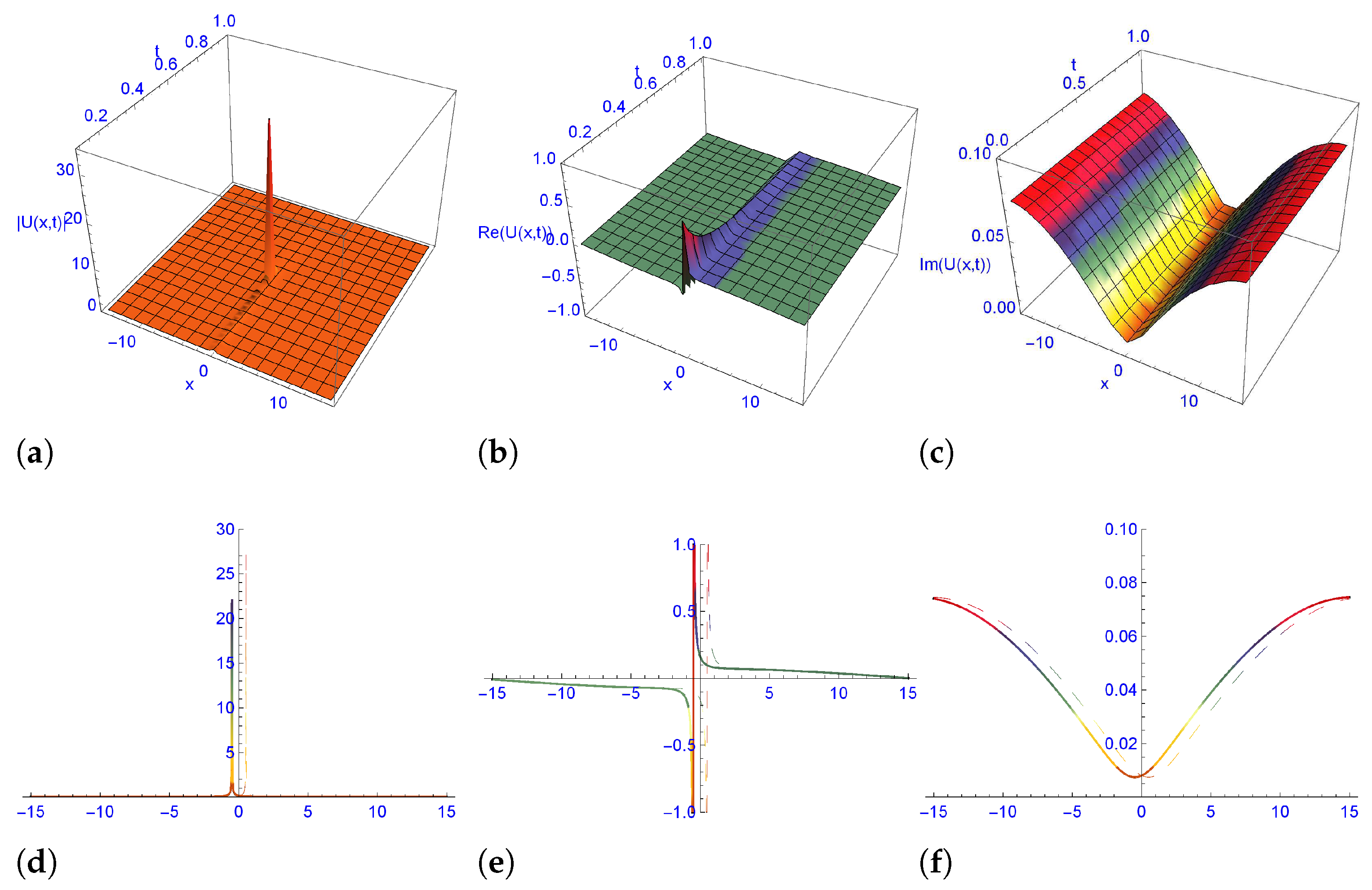
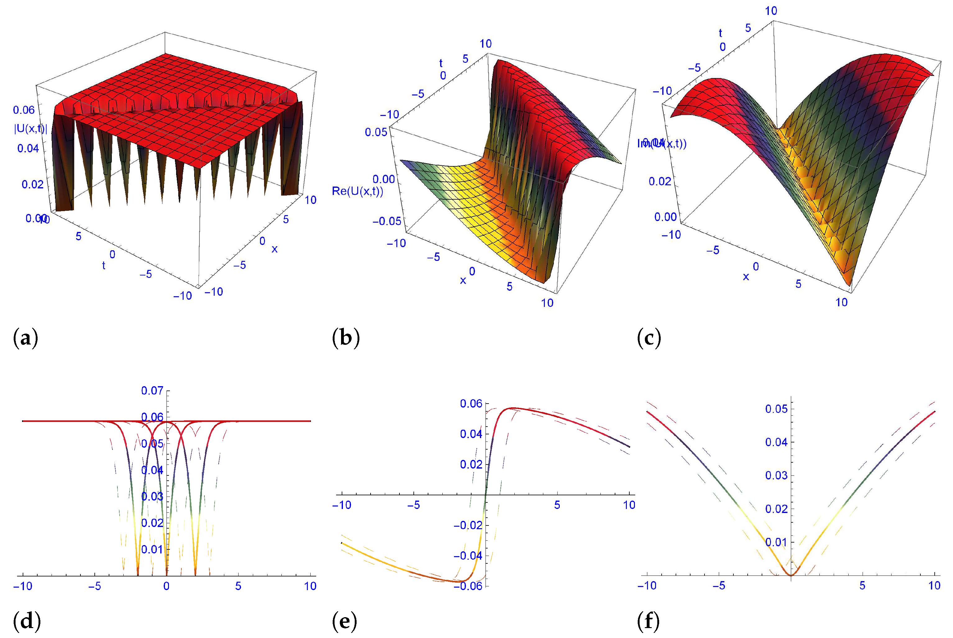
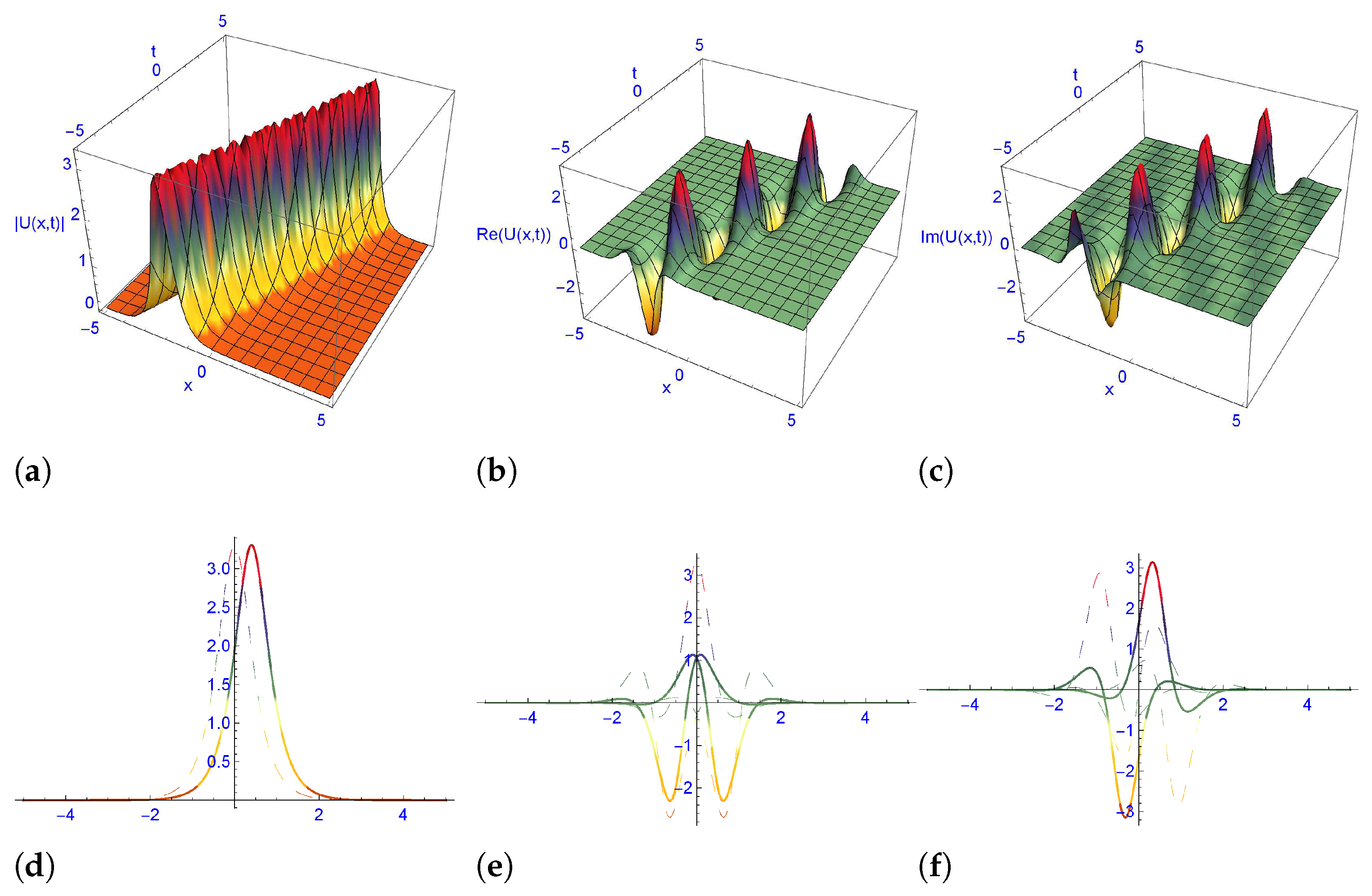
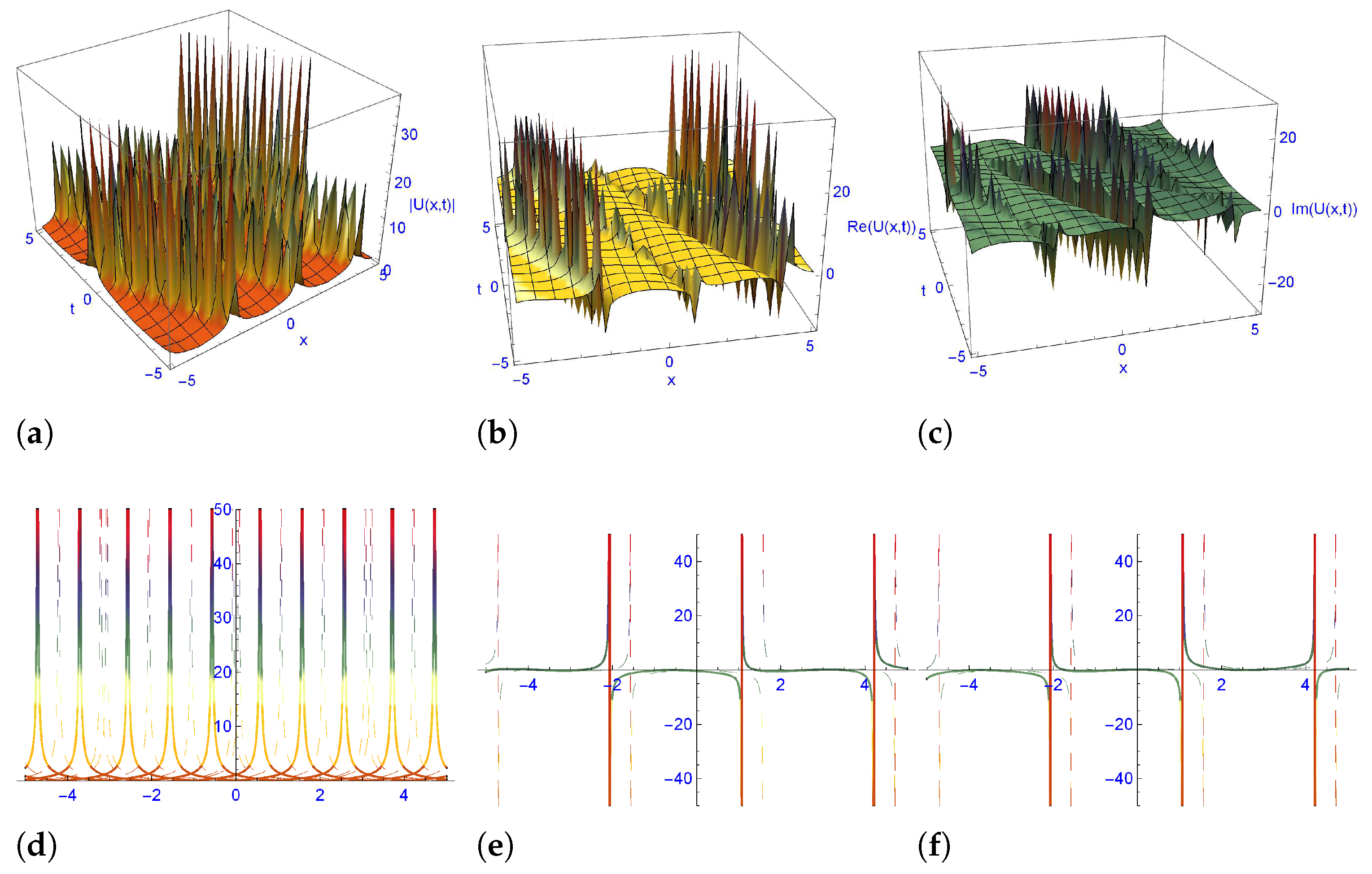
5. Physical Interpretation

It has been seen that the obtained solutions of UNLSE and mUNLSE using the currently suggested method, which is the improved auxiliary equation method, are different from those obtained by using alternative methods. Our findings are innovative and straightforward. The noticeable features of obtaining the results of the proposed method are unique a structure of solutions and Equation (7), which produce distinct solutions. Some works on unstable NLSEs and their exact wave solutions are as follows. The UNLSE was solved by utilizing the modified extended mapping method [53]. The $(G^{\prime }/G)$-expansion scheme was used in [54] to obtain wave results for the UNLSE. Researchers in [28] used the extended simple equation technique to construct the exact solutions of unstable and modified unstable NLSEs. The modified exponential rational function technique was used by the researchers in [55] to obtain traveling wave results of UNLSE and mUNLSE. The extended mapping method was used by author [56] for solutions of mUNLSE. Therefore, we have accomplished many ingenious results that have not been stated before.

The suggested approach has produced a number of wave solutions in the mode of special Jacobi elliptic, trigonometric, and hyperbolic functions; all of them have important applications in applied sciences. Furthermore, with the assistance of the suitable parameter values, various kinds of bright-dark, multi-wave structures, breather and kink-type solitons, and several periodic solitary waves structures are obtained that aid in the comprehension understanding of nonlinear models. Figure 1, Figure 2, Figure 3 and Figure 4 illustrate the solitary waves solutions in different shapes of UNLSE. In Figure 1, the waves solution (19) in different architectures is drawn with the help of relevant parameters: (a) the kink-type soliton with its 2D in (d), combine dark-bright solitary waves in (b) and (c), and their 2D in (e) and (f). In Figure 2, the waves solution (22) in different architectures is drawn with the help of relevant parameters: (a) is multi peaks mixed waves with its 2D in (d), (b) is Breather-type waves of a strange structure with its 2D in (e), and (c) is the periodic soliton with its 2D in (f). In Figure 3, the waves solution (26) in different architectures is drawn with the help of relevant parameters: (a) is Bright solitons and its 2D in (d), (b) and (c) are multi-peakon solitons that have different amplitude with their 2D in (e) and (f). In Figure 4, the waves solution (48) in different architectures is drawn with the help of relevant parameters: (a) the periodic bright-dark solitary wave with its 2D in (d), (b), and (c) are Breather-type waves of strange shapes and their 2D in (e) and (f).

Figure 5, Figure 6, Figure 7 and Figure 8 illustrate the solitary wave solutions in various shapes of (mULSE). In Figure 5, the waves solution (36) in different architectures is drawn with the help of relevant parameters: (a) A Peakon soliton of amplitude 30 with its 2D in (d), (b) is a dark-bright solitary wave with its 2D in (e), and (c) is a dark solitary wave with its 2D in (f). Similarly, in Figure 6, the waves solution (39) in different architectures is drawn with the help of relevant parameters: (a) the multi-peak soliton with its 2D in (d), (b) is the Kink type solitary wave with its 2D in (e), and (c) is the dark soliton with its 2D in (f). In Figure 7, the waves solution (46) in different architectures is drawn with the help of relevant parameters: (a) is the Bright soliton with its 2D in (d), and (b) and (c) are multi peakon solitons with their 2D in (e) and (f). In Figure 8, the waves solution (48) in different architectures is drawn with the help of relevant parameters: (a), (b) and (c) are Kinky-breathers-type wave structures with their 2D in (d), (e), and (f), respectively.

6. Conclusions

The suggested improved auxiliary equation approach has been effectively used in this study to obtain innovative wave solutions of UNLSEs. These unstable nonlinear Schrödinger equations are universal equations of the nonlinear integrable system class that depict the temporal evolution of disruption in slightly stable or unstable mediums. Numerous varieties of results are generated in the form of the Jacobi elliptic function, and trigonometric and hyperbolic functions, many of which are distinctive and have significant applications in the fields of applied sciences and mathematical physics. Moreover, with the assistance of the suitable parameter values, various kinds of bright-dark, multi-wave structures, breather and kink-type solitons, and several periodic solitary waves are plotted, which help to describe the physical interpretation of unstable nonlinear equations models. The various constructed solutions demonstrate the utility of the suggested approach, which proves that the proposed technique can be utilized in other non-linear physical models occurring in mathematical physics.

References

1. Mitschke, F.; Mahnke, C.; Hause, A. Soliton Content of Fiber-Optic Light Pulses. Appl. Sci. 2017, 7, 635. [Google Scholar] [CrossRef]
2. Chabchoub, A.; Kibler, B.; Finot, C.; Millot, G.; Onorato, M.; Dudley, J.M.; Babanin, A.V. The nonlinear Schrödinger equation and the propagation of weakly nonlinear waves in optical fibers and on the water surface. Ann. Phys. 2015, 361, 490–500. [Google Scholar] [CrossRef]
3. Kumar, S.; Kumar, A.; Wazwaz, A.-M. New exact solitary wave solutions of the strain wave equation in microstructured solids via the generalized exponential rational function method. Eur. Phys. J. Plus 2020, 135, 870. [Google Scholar] [CrossRef]
4. Arshad, M.; Seadawy, A.R.; Lu, D. Modulation stability and dispersive optical soliton solutions of higher order nonlinear Schrödinger equation and its applications in mono-mode optical fibers. Superlattices Microstruct. 2018, 113, 419–429. [Google Scholar] [CrossRef]
5. Akbar, M.A.; Ali, N.; Wazwaz, A.M. Closed form traveling wave solutions of non-linear fractional evolution equations through the modified simple equation method. Therm. Sci. 2018, 22, 341352. [Google Scholar]
6. Yin, H.M.; Pan, Q.; Chow, K.W. Doubly periodic solutions and breathers of the Hirota equation: Recurrence, cascading mechanism and spectral analysis. Nonlinear Dyn. 2022, 110, 3751–3768. [Google Scholar] [CrossRef]
7. Yin, H.M.; Chow, K.W. Breathers, cascading instabilities and Fermi-Pasta-Ulam-Tsingou recurrence of the derivative nonlinear Schrödinger equation: Effects of ‘self-steepening’ nonlinearity. Phys. D 2021, 428, 133033. [Google Scholar] [CrossRef]
8. Frassu, S.; Galván, R.R.; Viglialoro, G. Uniform in time L-estimates for an attraction-repulsion chemotaxis model with double saturation. Discrete Contin. Dyn. Syst. Ser. B 2023, 3, 1886–1904. [Google Scholar] [CrossRef]
9. Frassu, S.; Li, T.; Viglialoro, G. Improvements and generalizations of results concerning attraction-repulsion chemotaxis models. Math. Methods Appl. Sci. 2022, 45, 11067–11078. [Google Scholar] [CrossRef]
10. Dvornikov, M. Stable Langmuir solitons in plasma with diatomic ions. Nonlin. Process. Geophys. 2013, 20, 581–588. [Google Scholar] [CrossRef] [Green Version]
11. He, J.S.; Charalampidis, E.G.; Kevrekidis, P.G.; Frantzeskakis, D.J. Rogue waves in nonlinear Schrödinger models with variable coefficients: Application to Bose–Einstein condensates. Phys. Lett. A 2014, 378, 577–583. [Google Scholar] [CrossRef]
12. Bona, J.L.; Saut, J.-C. Dispersive Blow-Up II. Schrödinger-Type Equations, Optical and Oceanic Rogue Waves. Chin. Ann. Math. Ser. B 2010, 31, 793–818. [Google Scholar] [CrossRef]
13. Grinevich, P.G.; Santini, P.M. The exact rogue wave recurrence in the NLS periodic setting via matched asymptotic expansions, for 1 and 2 unstable modes. Phys. Lett. A 2018, 382, 973–979. [Google Scholar] [CrossRef] [Green Version]
14. Chabchoub, A.; Grimshaw, R.H.J. The Hydrodynamic Nonlinear Schrödinger Equation: Space and Time. Fluids 2016, 1, 23. [Google Scholar] [CrossRef] [Green Version]
15. Kumar, S.; Kumar, D.; Kharbanda, H. Lie symmetry analysis, abundant exact solutions and dynamics of multisolitons to the (2 + 1)-dimensional KP-BBM equation. Pramana 2021, 95, 33. [Google Scholar] [CrossRef]
16. Yin, H.M.; Pan, Q.; Chow, K.W. Four-wave mixing and coherently coupled Schrödinger equations: Cascading processes and Fermi–Pasta–Ulam–Tsingou recurrence. Chaos 2021, 31, 083117. [Google Scholar] [CrossRef]
17. Solli, D.R.; Ropers, C.; Koonath, P.; Jalali, B. Optical rogue waves. Nature 2007, 450, 1054–1057. [Google Scholar] [CrossRef]
18. Viotti, C.; Dutykh, D.; Dudley, J.M.; Dias, F. Emergence of coherent wave groups in deep-water random sea. Phys. Rev. E 2013, 87, 063001. [Google Scholar] [CrossRef] [Green Version]
19. Kumar, S.; Kumar, D.; Kumar, A. Lie symmetry analysis for obtaining the abundant exact solutions, optimal system and dynamics of solitons for a higher-dimensional Fokas equation. Chaos Solitons Fractals 2021, 142, 110507. [Google Scholar] [CrossRef]
20. Khatun, M.A.; Arefin, M.A.; Uddin, M.H.; Baleanu, D.; Akbar, M.A.; Inc, M. Explicit wave phenomena to the couple type fractional order nonlinear evolution equations. Results Phys. 2021, 28, 104597. [Google Scholar] [CrossRef]
21. Kibler, B.; Fatome, J.; Finot, C.; Millot, G.; Dias, F.; Genty, G.; Akhmediev, N.; Dudley, J.M. The Peregrine soliton in nonlinear fibre optics. Nat. Phys. 2010, 6, 790–795. [Google Scholar] [CrossRef]
22. Frisquet, B.; Kibler, B.; Millot, G. Collision of Akhmediev Breathers in Nonlinear Fiber Optics. Phys. Rev. X 2013, 3, 041032. [Google Scholar] [CrossRef] [Green Version]
23. Chabchoub, A.; Hoffmann, N.; Onorato, M.; Akhmediev, N. Super Rogue Waves: Observation of a Higher-Order Breather in Water Waves. Phys. Rev. X 2012, 2, 011015. [Google Scholar] [CrossRef] [Green Version]
24. Zakharov, V.E.; Ostrovsky, L.A. Modulation instability: The beginning. Phys. D 2009, 238, 540–548. [Google Scholar] [CrossRef]
25. Hosseini, K.; Mirzazadeh, M.; Baleanu, D.; Salahshour, S.; Akinyemi, L. Optical solitons of a high-order nonlinear Schrödinger equation involving nonlinear dispersions and Kerr effect. Opt. Quantum Electron. 2022, 54, 177. [Google Scholar] [CrossRef]
26. Habib, M.A.; Ali, H.M.S.; Miah, M.M.; Akbar, M.A. The generalized Kudryashov method for new closed form traveling wave solutions to some NLEEs. AIMS Math. 2019, 4, 896–909. [Google Scholar] [CrossRef]
27. Arshad, M.; Seadawy, A.R.; Lu, D. Optical soliton solutions of the generalized higher-order nonlinear Schrödinger equations and their applications. Opt. Quantum Electron. 2017, 49, 421. [Google Scholar] [CrossRef]
28. Lu, D.; Seadawy, A.R.; Arshad, M. Applications of extended simple equation method on unstable nonlinear Schrödinger equations. Optik 2017, 140, 136–144. [Google Scholar] [CrossRef]
29. Elboree, M.K. The Jacobi elliptic function method and its application for two component BKP hieracy equations. Comput. Math. Appl. 2011, 62, 4402–4414. [Google Scholar] [CrossRef] [Green Version]
30. Khan, K.; Akbar, M.A.; Islam, M. Exact solutions for (1 + 1)-dimensional nonlinear dispersive modified Benjamin-Bona-Mahony equation and coupled Klein-Gordon equations. SpringerPlus 2014, 3, 724. [Google Scholar] [CrossRef] [Green Version]
31. Arshad, M.; Seadawy, A.R.; Lu, D. Modulation stability and optical soliton solutions of nonlinear Schrödinger equation with higher order dispersion and nonlinear terms and its applications. Superlattices Microstruct. 2017, 112, 422–434. [Google Scholar] [CrossRef]
32. Biswa, A.; Arshed, S. Application of semi-inverse variational principle to cubic-quartic optical solitons with kerr and power law nonlinearity. Optik 2018, 172, 847–850. [Google Scholar] [CrossRef]
33. Gaber, A.A.; Aljohani, A.F.; Ebaid, A.; Machado, J.T. The generalized Kudryashov method for nonlinear space–time fractional partial differential equations of Burgers type. Nonlinear Dyn. 2019, 95, 361–368. [Google Scholar] [CrossRef]
34. Miah, M.M.; Ali, H.M.S.; Akbar, M.A.; Wazwaz, A.M. Some applications of the (G/G,1/G)-expansion method to find new exact solutions of NLEEs. Eur. Phys. J. Plus 2017, 132, 252. [Google Scholar] [CrossRef]
35. Zhang, R.-F.; Li, M.-C. Bilinear residual network method for solving the exactly explicit solutions of nonlinear evolution equations. Nonlinear Dyn. 2022, 108, 521–531. [Google Scholar] [CrossRef]
36. Seadawy, A.R.; Lu, D.; Khater, M.M.A. Bifurcations of traveling wave solutions for Dodd-Bullough-Mikhailov equation and coupled Higgs equation and their applications. Chin. J. Phys. 2017, 55, 1310–1318. [Google Scholar] [CrossRef]
37. Yasar, E.; Yildirim, Y.; Yasar, E. New optical solitons of space-time conformable fractional perturbed Gerdjikov-Ivanov equation by sine-Gordon equation method. Results Phys. 2018, 9, 1666–1672. [Google Scholar] [CrossRef]
38. Hosseini, M.M.; Ghaneai, H.; Mohyud-din, S.T.; Usman, M. Tri-prong scheme for regularized long wave equation. J. Assoc. Arab Univ. Basic Appl. Sci. 2016, 20, 68–77. [Google Scholar] [CrossRef]
39. Yin, H.M.; Pan, Q.; Chow, K.W. The Fermi–Pasta–Ulam–Tsingou recurrence for discrete systems: Cascading mechanism and machine learning for the Ablowitz-Ladik equation. Commun. Nonlinear Sci. Numer. Simul. 2022, 114, 106664. [Google Scholar] [CrossRef]
40. Yang, Y.; Suzuki, T.; Cheng, X. Darboux transformations and exact solutions for the integrable nonlocal Lakshmanan-Porsezian-Daniel equation. Appl. Math. Lett. 2020, 99, 105998. [Google Scholar] [CrossRef]
41. Fang, J.; Wu, B.; Liu, W. An explicit spectral collocation method for the linearized Korteweg–de Vries equation on unbounded domain. Appl. Numer. Math. 2018, 126, 34–52. [Google Scholar] [CrossRef]
42. Zeng, X.; Wang, D.S. A generalized extended rational expansion method and its application to (1 + 1)-dimensional dispersive long wave equation. Appl. Math. Comput. 2009, 212, 296–304. [Google Scholar] [CrossRef]
43. Wang, Y.-H.; Chen, Y. Binary Bell Polynomials, Bilinear Approach to Exact Periodic Wave Solutions of (2 + 1)-Dimensional Nonlinear Evolution Equations. Commun. Theor. Phys. 2011, 56, 672–678. [Google Scholar] [CrossRef] [Green Version]
44. Rizea, M. Exponential fitting method for the time-dependent Schrödinger equation. J. Math. Chem. 2010, 48, 55–65. [Google Scholar] [CrossRef]
45. Zayed, E.M.E.; Alurrfi, K.A.E. New extended auxiliary equation method and its applications to nonlinear Schrödinger-type equations. Optik 2016, 127, 9131–9151. [Google Scholar] [CrossRef]
46. Sarwar, A.; Gang, T.; Arshad, M.; Ahmed, I. Construction of brightdark solitary waves and elliptic function solutions of space-time fractional partial differential equations and their applications. Phys. Scr. 2020, 95, 045227. [Google Scholar] [CrossRef]
47. Nasreen, N.; Lu, D.; Arshad, M. Optical soliton solutions of nonlinear Schrödinger equation with second order spatiotemporal dispersion and its modulation instability. Optik 2018, 161, 221–229. [Google Scholar] [CrossRef]
48. Kumar, S.; Ma, W.-X.; Kumar, A. Lie symmetries, optimal system and group-invariant solutions of the (3 + 1)-dimensional generalized KP equation. Chin. J. Phys. 2021, 69, 1–23. [Google Scholar] [CrossRef]
49. Hafiz Uddin, M.; Zaman, U.H.M.; Arefin, M.A.; Akbar, M.A. Nonlinear dispersive wave propagation pattern in optical fiber system. Chaos Solitons Fractals 2022, 164, 112596. [Google Scholar] [CrossRef]
50. Pedlosky, J. Finite-amplitude baroclinic waves. J. Atmos. Sci. 1970, 27, 15–30. [Google Scholar] [CrossRef]
51. Pawlik, M.; Rowlands, G. The propagation of solitary waves in piezoelectric semiconductors. J. Phys. C Solid State Phys. 1975, 8, 1189–1204. [Google Scholar] [CrossRef]
52. Wadati, M.M.; Segur, H.; Ablowitz, M.J. A new Hamiltonian amplitude equation governing modulated wave instabilities. J. Phys. Soc. Jpn. 1992, 61, 1187–1193. [Google Scholar] [CrossRef]
53. Arshad, M.; Seadawy, A.R.; Lu, D.; Jun, W. Optical soliton solutions of unstable nonlinear Schrödinger dynamical equation and stability analysis with applications. Optik 2018, 157, 597–605. [Google Scholar] [CrossRef]
54. Arbabi, S.; Najafi, M. Exact solitary wave solutions of the complex nonlinear Schrödinger equations. Optik 2016, 127, 4682–4688. [Google Scholar] [CrossRef]
55. Yue, L.; Lu, D.; Arshad, M.; Xu, X. New exact traveling wave solutions of the unstable nonlinear Schrödinger equations and their applications. Optik 2021, 226, 165386. [Google Scholar]
56. Arshad, M.; Seadawy, A.R.; Lu, D.; Jun, W. Modulation instability analysis of modify unstable nonlinear Schrödinger dynamical equation and its optical soliton solutions. Results Phys. 2017, 7, 4153–4161. [Google Scholar] [CrossRef]
Figure 1. The solutions (19) are drawn in different shapes at c 0 = a 0 = 0.1 , a 2 = 1.5 , a 4 = 0.1 , κ = λ = μ = σ = τ = 1 : (a) Kink-type soliton with its 2D in (d), combining dark-bright solitary waves in (b) and (c), and their 2D in (e) and (f), respectively.
Symmetry 15 00099 g001
Figure 2. The solutions (22) are drawn in different shapes at: (a) is multi peaks mixed waves with its 2D in (d), (b) is Breather-type waves of strange structure with its 2D in (e), and (c) is periodic soliton with its 2D in (f), respectively, at c 0 = a 0 = 0.1 , a 2 = 1.25 , a 4 = 0.1 , κ = λ = μ = σ = τ = 1 .
Symmetry 15 00099 g002
Figure 3. The solution (26) in different shapes are drawn at γ = μ = 0.1 , σ = 1.5 , κ = λ = ν = 1 = τ = 1 : (a) is Bright solitons, and its 2D in (bd) are multi-peakon solitons that have different amplitudes with their 2D in (e) and (f), respectively.
Symmetry 15 00099 g003
Figure 4. The solution (28) in different shapes is drawn at γ = μ = 0.1 , σ = 0.1 , κ = λ = ν = 1 = τ = 1 : (a) Periodic bright-dark solitary wave with its 2D in (bd) are Breather-type waves of strange shapes and their 2D in (e) and (f), respectively.
Symmetry 15 00099 g004
Figure 5. The solution (36) in different shapes is drawn at c 2 = 0.5 , a 0 = a 4 = 0.1 , a 2 = 0.35 , ρ = ω = 0.1 , τ = κ = λ = 1 : (a) Peakon soliton with its 2D in (d), (b) is dark-bright solitary wave with its 2D in (e), and (c) is dark solitary wave with its 2D in (f), respectively.
Symmetry 15 00099 g005
Figure 6. The solution (39) in different shapes are drawn at c 2 = 1.75 , a 0 = a 4 = 0.1 , a 2 = τ = 1.5 , ρ = ω = 0.1 , κ = λ = 1 : (a) Multi-peak dark soliton with its 2D in (d), (b) Kink type solitary wave with its 2D in (e), and (c) dark soliton with its 2D in (f), respectively.
Symmetry 15 00099 g006
Figure 7. The solution (46) in different shapes is drawn at c 1 = 1.5 , a 2 = 1.25 , ρ = 2.5 , γ = ω = ν = τ = 1 , κ = 2.5 , λ = 1 : (a) is Bright soliton with its 2D in (bd) are multi-peakon solitons with their 2D in (e) and (f), respectively.
Symmetry 15 00099 g007
Figure 8. The solution (48) in different shapes is drawn at ρ = 1.5 , γ = ω = ν = τ = 1 , κ = 2 , λ = 1 : (ac) are Kinky-breathers-type wave structures with their 2D in (df), respectively.
Symmetry 15 00099 g008
Disclaimer/Publisher’s Note: The statements, opinions and data contained in all publications are solely those of the individual author(s) and contributor(s) and not of MDPI and/or the editor(s). MDPI and/or the editor(s) disclaim responsibility for any injury to people or property resulting from any ideas, methods, instructions or products referred to in the content.