Article

Construction of Solitary Wave Solutions to the (3 + 1)-Dimensional Nonlinear Extended and Modified Quantum Zakharov–Kuznetsov Equations Arising in Quantum Plasma Physics

1
Department of Mathematics, Faculty of Science, University of Tabuk, P.O. Box 741, Tabuk 71491, Saudi Arabia
2
Mathematics Department, Faculty of Science, Taibah University, P.O. Box 344, Al-Madinah Al-Munawarah 41411, Saudi Arabia
3
Department of Mathematics, University of Education, Multan Campus, Lahore 54000, Pakistan
4
Department of Mathematics, Faculty of Sciences, King Abdulaziz University, Jeddah 21589, Saudi Arabia
*
Author to whom correspondence should be addressed.
Symmetry 2023, 15(1), 248; https://doi.org/10.3390/sym15010248
Submission received: 26 November 2022 / Revised: 6 January 2023 / Accepted: 13 January 2023 / Published: 16 January 2023

Abstract

:
Several types of solitary wave solutions of (3 + 1)-dimensional nonlinear extended and modified quantum Zakharov–Kuznetsov equations are established successfully via the implantation of three mathematical methods. The concerned models have many fruitful applications to describe the waves in quantum electron–positron–ion magnetoplasmas and weakly nonlinear ion-acoustic waves in plasma. The derived results via the MEAEM method, ESE method, and modified F-expansion have been retrieved and will be expedient in the future to illuminate the collaboration between lower nonlinear ion-acoustic waves. For the physical behavior of the models, some solutions are plotted graphically in 2D and 3D by imparting particular values to the parameters under the given condition at each solution. Hence explored solutions have profitable rewards in the field of mathematical physics.

1. Introduction

A developing concentration has been engrossed in the research of analytical and numerical solutions of nonlinear evolutions equations (NLEEs) during the previous eras [1,2,3,4,5,6]. NLEEs are used to demonstrate phenomena in dissimilar fields of science and engineering such as optic fibers, plasmas, biology, fluid mechanics, acoustics, and numerous others [7,8,9,10,11,12,13,14,15,16,17,18,19,20,21,22]. Exact and solitary wave solutions of NLEEs were made possible with the initiation of the selection of mathematical tools [8,9,10,11,12,13,14,15,16,17,18,19,20,21,22,23,24,25,26,27,28,29,30,31]. Currently, diverse categories of nonlinear evolution equations were developed using a powerful reductive perturbation technique or a multiscale analysis [32,33,34,35]. Further specifically, the exploration of exact solutions called soliton-like solutions has advanced quickly today, which is one of the significant topics of nonlinear science. Solitons have enormous features because of their stuff (stability, robustness, and the ability to preserve their velocity and shape after interaction) [18,19,20,21,22], and they occur in various forms such as bright, dark, kink, pulses, breather, and so on. Furthermore, lately, novel forms of bright and dark solitons known as W-shape and M-shape have been exposed. A similar number of works have been approved to show the relevance of these results [36,37,38,39,40]. However, searching for the exact traveling wave solutions still poses a problem at times due to not all the known methods can be applied to NLEEs. In this current research, we explore solitary wave solutions by applying three mathematical methods, modified extended auxiliary equation mapping method, extended simple equation method, and modified F-expansion method [41,42]. The derived solutions have great potential to handle nonlinear problems in mathematical physics.
The article is arranged as follows: Section 2 is a survey of the proposed schemes. Section 3 is an implementation of the presented methods to concern models. The obtained solitary wave solutions to the (3 + 1)-Dimensional nonlinear extended and modified quantum Zakharov–Kuznetsov equations are given in Section 4. Section 5 gives the results and summary of the work.

2. Description of the Methods

Let the NPDE has a form as
E U , U t , U x , U x x , U x t , = 0 .
Let
U = U ( ξ ) , ξ = k x ω t .
Substitute (2) in (1),
F U , U , U , = 0 .

2.1. Modified Extended Auxiliary Equation Mapping Method

Suppose the solution of (3) is,
U = i = 0 N A i Ψ i + i = 1 N B i Ψ i + i = 2 N C i Ψ i 2 Ψ + i = 1 N D i Ψ Ψ i .
Let Ψ satisfy,
Ψ = β 1 Ψ 2 + β 2 Ψ 3 + β 3 Ψ 4 .
Put (4) with (5) in (3), we found the solution of (1).

2.2. Extended Simple Equation Method

Let (3) has solution,
U ( ξ ) = i = N N A i Ψ i ( ξ ) .
Let Ψ satisfy,
Ψ = c 0 + c 1 Ψ + c 2 Ψ 2 + c 3 Ψ 3 .
Put (6) with (7) in (3). We get the solution of (1).

2.3. Modified F-Expansion Method

Suppose the solution of (3) is:
U = a 0 + i = 1 N a i F i ( ξ ) + i = 1 N b i F i ( ξ ) .
Let F obliges,
F = A + B F + C F 2 .
Put (8) with (9) in (3). Solve obtained system to establish the required solution of (1).

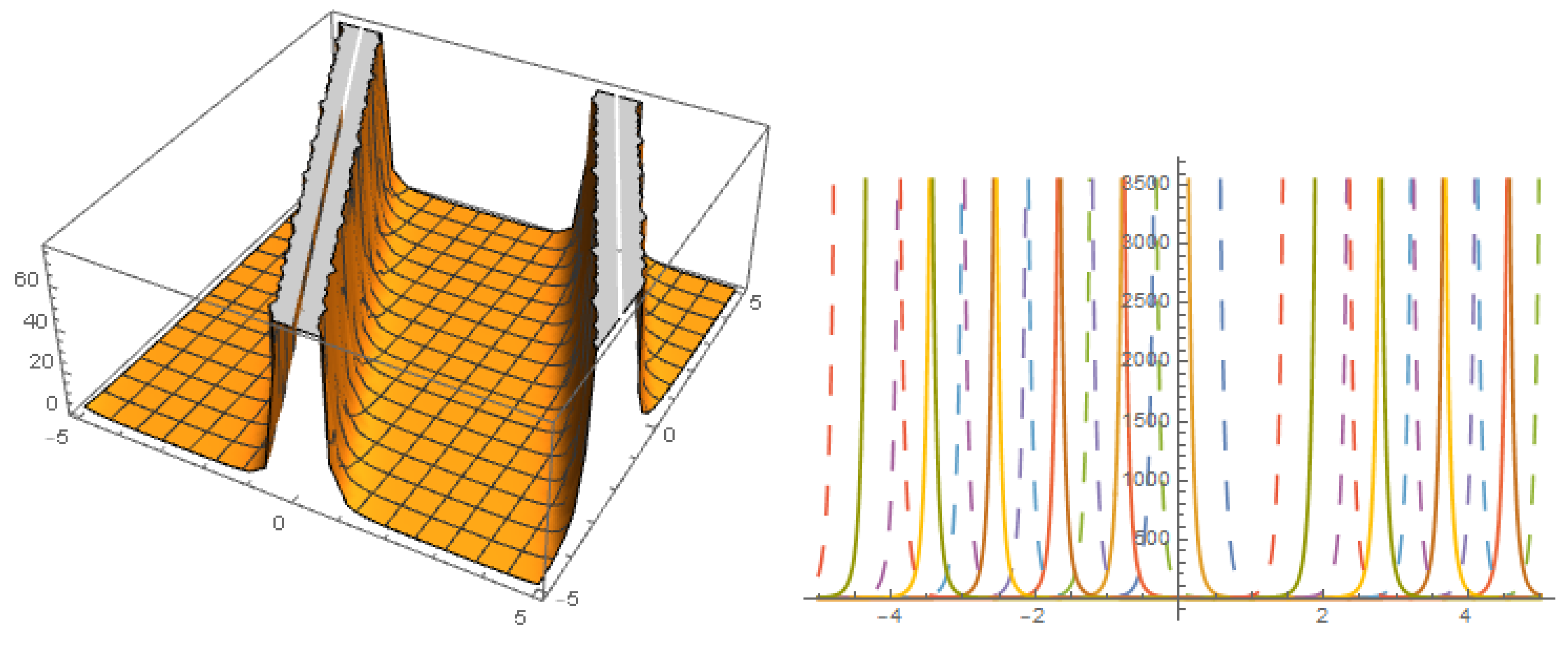
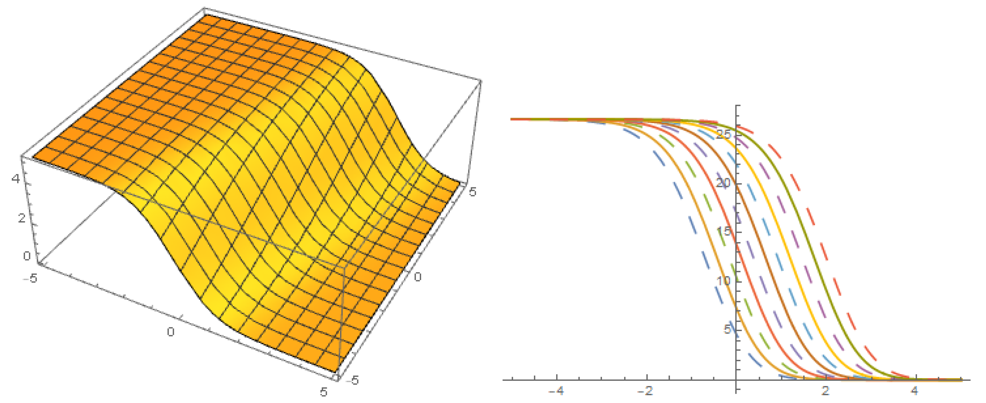
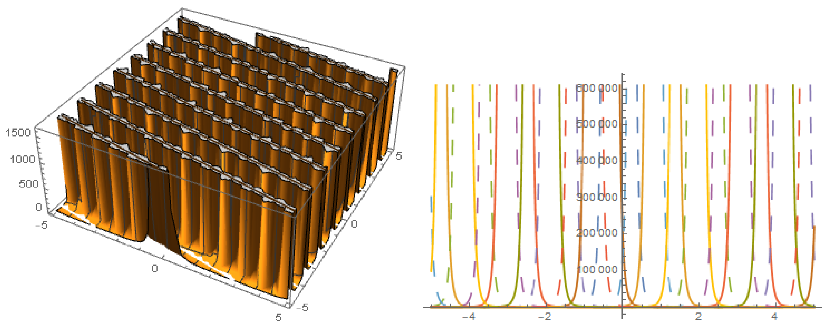
3. (3 + 1)-Dimensional Nonlinear Extended Quantum Zakharov–Kuznetsov (NLEQZK) Equation

Let NLEQZK equation [36,38,39].
U t + PU + QU 2 U z + R 3 U z 3 + S z 2 x 2 + 2 y 2 U = 0 .
The (3 + 1)-dimensional NLEQZK model has fruitful applications to handle the quantum electron-positron-ion magneto-plasmas, warm ions, and hot isothermal electrons in the existence of a uniform magnetic field.
Let wave transformations,
U ( x , y , z , t ) = U ( ξ ) , ξ = α x + β y + γ z ω t .
Put (11) in (10), after integrating and omitting the integral constant, we have
1 2 γ P U 2 + 1 3 γ Q U 3 + U γ 3 R + γ S α 2 + β 2 U ω = 0 .

3.1. Application of Modified Extended Auxiliary Equation Mapping Method

Let solution of (12) is,
U = A 1 Ψ + A 0 + B 1 Ψ + D 1 Ψ Ψ .
Put (13) with (5) in (12), we obtained the coefficients of solutions as following
A 0 = P 2 Q , A 1 = β 3 P 2 β 1 Q , B 1 = 0 , D 1 = P 2 β 1 Q , ω = γ P 2 6 Q , α = P 2 6 β 1 γ 2 Q R 6 β 2 β 1 Q S 6 β 1 Q S .
Substitute (14) in (13), we found the solutions of Equation (10)
CASE I:
U 1 = β 3 P β 1 ϵ coth 1 2 β 1 ξ + ξ 0 + 1 β 2 2 β 1 Q + P β 1 3 / 2 ϵ csc h 2 1 2 β 1 ξ + ξ 0 2 β 1 Q 2 β 2 β 1 ϵ coth 1 2 β 1 ξ + ξ 0 + 1 β 2 P 2 Q , β 1 > 0 , β 2 2 4 β 1 β 3 = 0 .
CASE II:
U 2 = P β 1 β 3 β 1 ϵ cosh β 1 ξ + ξ 0 cosh β 1 ξ + ξ 0 + η β 1 ϵ sinh 2 β 1 ξ + ξ 0 cosh β 1 ξ + ξ 0 + η 2 2 β 1 Q 2 β 1 4 β 3 ϵ sinh β 1 ξ + ξ 0 cosh β 1 ξ + ξ 0 + η + 1 β 3 P β 1 4 β 3 ϵ sinh β 1 ξ + ξ 0 cosh β 1 ξ + ξ 0 + η + 1 2 β 1 Q P 2 Q , β 1 > 0 , β 3 > 0 , β 2 = 4 β 1 β 3 1 / 2 .
CASE III:
U 3 = P β 1 β 1 ϵ cosh β 1 ξ + ξ 0 cosh β 1 ξ + ξ 0 + η P 2 + 1 β 1 ϵ sinh β 1 ξ + ξ 0 sinh β 1 ξ + ξ 0 + P cosh β 1 ξ + ξ 0 + η P 2 + 1 2 2 β 1 Q β 2 β 1 ϵ sinh β 1 ξ + ξ 0 + P cosh β 1 ξ + ξ 0 + η P 2 + 1 + 1 β 2 P 2 Q + β 3 P 2 β 1 Q β 1 ϵ sinh β 1 ξ + ξ 0 + P cosh β 1 ξ + ξ 0 + η P 2 + 1 + 1 β 2 , β 1 > 0 .
Some solutions are plotted graphically in 2-dimensional and 3-dimensional by imparting particular value to the parameters under the constrain condition on each disquiet solution (Figure 1, Figure 2, Figure 3, Figure 4, Figure 5, Figure 6, Figure 7, Figure 8, Figure 9, Figure 10 and Figure 11).

3.2. Application of Extended Simple Equation Method

Let solution of (12) is
U = A 1 Ψ + A 1 Ψ + A 0 .
Put (18) with (7) in (12), we derived the coefficients as following
CASE 1: c 3 = 0 ,
FAMILY-I
A 1 = 0 , A 1 = c 2 P c 1 2 Q 2 4 c 0 c 2 Q 2 , A 0 = c 1 P Q c 1 2 4 c 0 c 2 Q 2 P 2 Q , ω = γ P 2 6 Q , α = 6 γ 2 c 1 2 Q R + 24 γ 2 c 0 c 2 Q R 6 β 2 c 1 2 Q S + 24 β 2 c 0 c 2 Q S P 2 6 c 1 2 Q S 24 c 0 c 2 Q S .
Put (19) in (18),
U 4 = c 2 P c 1 4 c 2 c 0 c 1 2 tan 1 2 4 c 2 c 0 c 1 2 ξ + ξ 0 2 c 2 c 1 2 Q 2 4 c 0 c 2 Q 2 + P c 1 Q c 1 2 4 c 0 c 2 Q 2 1 2 Q , 4 c 0 c 2 > c 1 2 .
FAMILY-II
A 1 = c 0 P c 1 2 Q 2 4 c 0 c 2 Q 2 , A 1 = 0 , A 0 = c 1 P Q c 1 2 4 c 0 c 2 Q 2 P 2 Q , ω = γ P 2 6 Q , α = 6 γ 2 c 1 2 Q R + 24 γ 2 c 0 c 2 Q R 6 β 2 c 1 2 Q S + 24 β 2 c 0 c 2 Q S P 2 6 c 1 2 Q S 24 c 0 c 2 Q S .
Substitute (21) in (18),
U 5 = c 1 P Q c 1 2 4 c 0 c 2 Q 2 P 2 Q c 0 P c 1 2 Q 2 4 c 0 c 2 Q 2 c 1 4 c 2 c 0 c 1 2 tan 1 2 4 c 2 c 0 c 1 2 ξ + ξ 0 2 c 2 , 4 c 0 c 2 > c 1 2 .
CASE 2: c 0 = 0 , c 3 = 0 ,
A 1 = 0 , A 1 = c 2 P c 1 Q , A 0 = P Q , ω = γ P 2 6 Q , α = 6 γ 2 c 1 2 Q R 6 β 2 c 1 2 Q S P 2 6 c 1 Q S .
Put (23) in (18),
U 6 = c 2 P c 1 exp c 1 ξ + ξ 0 c 1 Q 1 c 2 exp c 1 ξ + ξ 0 P Q , c 1 > 0 ,
U 7 = c 2 P c 1 exp c 1 ξ + ξ 0 c 1 Q c 2 exp c 1 ξ + ξ 0 + 1 P Q , c 1 < 0 .
CASE 3: c 1 = 0 , c 3 = 0 ,
FAMILY-I
A 1 = 0 , A 1 = i c 2 P 2 c 0 Q , A 0 = P 2 Q , α = 24 γ 2 c 0 c 2 Q R 24 β 2 c 0 c 2 Q S + P 2 2 6 c 0 c 2 Q S , ω = γ P 2 6 Q .
Put (26) in (18),
U 8 = P 2 Q + i c 2 P c 0 c 2 tan c 0 c 2 ξ + ξ 0 c 2 2 c 0 Q , c 0 c 2 > 0 ,
U 9 = P 2 Q + i c 2 P c 0 c 2 tanh c 0 c 2 ξ + ξ 0 c 2 2 c 0 Q , c 0 c 2 < 0 .
FAMILY-II
A 1 = i c 0 P 2 c 2 Q , A 1 = 0 , A 0 = P 2 Q , α = 24 γ 2 c 0 c 2 Q R 24 β 2 c 0 c 2 Q S + P 2 2 6 c 0 c 2 Q S , ω = γ P 2 6 Q .
Put (29) in (18),
U 10 = P 2 Q + i c 0 P 2 c 2 Q c 0 c 2 tan c 0 c 2 ξ + ξ 0 c 2 , c 0 c 2 > 0 ,
U 11 = P 2 Q + i c 0 P 2 c 2 Q i c 2 P c 0 c 2 tanh c 0 c 2 ξ + ξ 0 c 2 2 c 0 Q ) , c 0 c 2 < 0 .
FAMILY-III
A 1 = c 0 P 2 2 c 2 Q , A 1 = c 2 P 2 2 c 0 Q , A 0 = P 2 Q , α = 48 γ 2 c 0 c 2 Q R 48 β 2 c 0 c 2 Q S P 2 4 3 c 0 c 2 Q S , ω = γ P 2 6 Q .
Put (32) in (18),
U 12 = c 2 P c 0 c 2 tan c 0 c 2 ξ + ξ 0 c 2 2 2 c 0 Q + c 0 P 2 2 c 2 Q c 0 c 2 tan c 0 c 2 ξ + ξ 0 c 2 P 2 Q , c 0 c 2 > 0 ,
U 13 = c 2 P c 0 c 2 tanh c 0 c 2 ξ + ξ 0 c 2 2 2 c 0 Q + c 0 P 2 2 c 2 Q c 0 c 2 tanh c 0 c 2 ξ + ξ 0 c 2 P 2 Q , c 0 c 2 < 0 .
Figure 2. Solution U 5 with β = 0.01 , c 0 = 1 , c 2 = 1 , c 1 = 0.01 , γ = 0.05 , ξ 0 = 3.5 , P = 4.5 , Q = 1.3 , R = 2.1 , S = 3.5 , ω = 2 , y = 1 , z = 1 .
Symmetry 15 00248 g002
Figure 3. Solution U 13 with β = 0.3 , c 0 = 1 , c 2 = 0.4 , γ = 0.9 , ξ 0 = 0.05 , P = 1.5 , Q = 1.3 , R = 1.5 , S = 0.3 , y = 1 , z = 1 .
Symmetry 15 00248 g003

3.3. Application of Modified F-Expansion Method

Let (12) has solution,
U = a 0 + a 1 F + b 1 F
Put (35) with (9) in (12).
A = 0, B = 1, C = −1,
a 1 = P Q , a 0 = P Q , b 1 = 0 , ω = γ P 2 6 Q , α = P 2 6 γ 2 Q R 6 β 2 Q S 6 Q S .
Put (36) in (35),
U 14 = P 1 2 tanh ξ 2 + 1 2 Q P Q .
A = 0, C = 1, B = −1,
a 1 = P Q , a 0 = 0 , b 1 = 0 , ω = γ P 2 6 Q , α = P 2 6 γ 2 Q R 6 β 2 Q S 6 Q S .
Put (38) into (35),
U 15 = P 1 2 1 2 coth ξ 2 Q .
A = 1/2, B = 0, C = −1/2
FAMILY-I
a 0 = a 1 = P 2 Q = P 2 Q , b 1 = 0 , ω = γ P 2 6 Q , α = P 2 6 γ 2 Q R 6 β 2 Q S 6 Q S .
Substitute (40) into (35),
U 16 , 1 = P ( cot ( ξ ) + csc ( ξ ) ) 2 Q P 2 Q .
FAMILY-II
a 1 = 0 , a 0 = P 2 Q , b 1 = P 2 Q , ω = γ P 2 6 Q , α = P 2 6 γ 2 Q R 6 β 2 Q S 6 Q S .
Put (42) in (35),
U 16 , 2 = P ( 2 Q ) ( cot ( ξ ) + csc ( ξ ) ) P 2 Q .
FAMILY-III
a 1 = P 4 Q , a 0 = P 2 Q , b 1 = P 4 Q , ω = γ P 2 6 Q , α = P 2 24 γ 2 Q R 24 β 2 Q S 2 6 Q S
Put (44) in (35),
U 16 , 3 = P ( cot ( ξ ) + csc ( ξ ) ) 4 Q P ( 4 Q ) ( cot ( ξ ) + csc ( ξ ) ) P 2 Q .
Figure 4. The profile of solution U 16 , 3 with β = 1 , γ = 3 , P = 1.01 , Q = 5.3 , R = 0.5 , S = 2.1 , y = 1 , z = 1 .
Symmetry 15 00248 g004
A = 1, B = 0, C = −1
FAMILY-I
a 1 = P 2 Q , a 0 = P 2 Q , b 1 = 0 , ω = γ P 2 6 Q , α = P 2 24 γ 2 Q R 24 β 2 Q S 2 6 Q S .
Put (46) in (35),
U 17 , 1 = P tanh ( ξ ) 2 Q P 2 Q .
FAMILY-II
a 1 = 0 , a 0 = P 2 Q , b 1 = P 2 Q , ω = γ P 2 6 Q , α = P 2 24 γ 2 Q R 24 β 2 Q S 2 6 Q S .
Put (48) in (35),
U 17 , 2 = P ( 2 Q ) tanh ( ξ ) P 2 Q .
FAMILY-III
a 1 = P 4 Q , a 0 = P 2 Q , b 1 = P 4 Q , ω = γ P 2 6 Q , α = P 2 96 γ 2 Q R 96 β 2 Q S 4 6 Q S .
Put (50) in (35),
U 17 , 3 = P tanh ( ξ ) 4 Q + P ( 4 Q ) tanh ( ξ ) P 2 Q .
A = C = 1/2, B = 0,
FAMILY-I
a 1 = i P 2 Q , a 0 = P 2 Q , b 1 = 0 , ω = γ P 2 6 Q , α = P 2 6 γ 2 Q R 6 β 2 Q S 6 Q S .
Put (52) in (35),
U 18 , 1 = P 2 Q ( i P ) ( tan ( ξ ) + sec ( ξ ) ) 2 Q .
FAMILY-II
a 1 = 0 , a 0 = P 2 Q , b 1 = i P 2 Q , ω = γ P 2 6 Q , α = P 2 6 γ 2 Q R 6 β 2 Q S 6 Q S .
Put (54) in (35),
U 18 , 2 = P 2 Q + i P ( 2 Q ) ( tan ( ξ ) + sec ( ξ ) ) .
FAMILY-III
a 1 = P 2 2 Q , a 0 = P 2 Q , b 1 = P 2 2 Q , ω = γ P 2 6 Q , α = P 2 12 γ 2 Q R 12 β 2 Q S 2 3 Q S .
Put (56) in (35),
U 18 , 3 = P ( tan ( ξ ) + sec ( ξ ) ) 2 2 Q + P 2 2 Q ( tan ( ξ ) + sec ( ξ ) ) P 2 Q .
A = C = −1/2, B = 0,
FAMILY-I
a 1 = i P 2 Q , a 0 = P 2 Q , b 1 = 0 , ω = γ P 2 6 Q , α = P 2 6 γ 2 Q R 6 β 2 Q S 6 Q S .
Put (58) in (35),
U 19 , 1 = P 2 Q ( i P ) ( sec ( ξ ) tan ( ξ ) ) 2 Q .
FAMILY-II
a 1 = 0 , a 0 = P 2 Q , b 1 = i P 2 Q , ω = γ P 2 6 Q , α = P 2 6 γ 2 Q R 6 β 2 Q S 6 Q S .
Put (60) in (35),
U 19 , 2 = P 2 Q i P ( 2 Q ) ( sec ( ξ ) tan ( ξ ) ) .
Figure 5. The profile of solution U 19 , 2 with β = 1 , γ = 3 , P = 1.01 , Q = 0.3 , R = 0.5 , S = 2.1 , y = 1 , z = 1 .
Symmetry 15 00248 g005
FAMILY-III
a 1 = P 2 2 Q , a 0 = P 2 Q , b 1 = P 2 2 Q , ω = γ P 2 6 Q , α = P 2 12 γ 2 Q R 12 β 2 Q S 2 3 Q S .
Put (62) in (35),
U 19 , 3 = P ( sec ( ξ ) tan ( ξ ) ) 2 2 Q P 2 2 Q ( sec ( ξ ) tan ( ξ ) ) P 2 Q .
A = C = −1, B = 0,
FAMILY-I
a 1 = i P 2 Q , a 0 = P 2 Q , b 1 = 0 , α = P 2 24 γ 2 Q R 24 β 2 Q S 2 6 Q S , ω = γ P 2 6 Q .
Put (64) in (35),
U 20 , 1 = P 2 Q ( i P ) tan ( ξ ) 2 Q .
FAMILY-II
a 1 = 0 , a 0 = P 2 Q , b 1 = i P 2 Q , α = P 2 24 γ 2 Q R 24 β 2 Q S 2 6 Q S , ω = γ P 2 6 Q .
Put (66) in (35),
U 20 , 2 = P 2 Q i P ( 2 Q ) tan ( ξ ) .
FAMILY-III
a 1 = P 2 2 Q , a 0 = P 2 Q , b 1 = P 2 2 Q , α = P 2 48 γ 2 Q R 48 β 2 Q S 4 3 Q S , ω = γ P 2 6 Q .
Put (68) in (35),
U 20 , 3 = P tan ( ξ ) 2 2 Q + P 2 2 Q tan ( ξ ) P 2 Q .
C = 0
a 1 = 0 , a 0 = 0 , b 1 = A P B Q , α = 6 B 2 γ 2 Q R 6 β 2 B 2 Q S P 2 6 B Q S , ω = γ P 2 6 Q .
Put (70) in (35),
U 21 = B ( A P ) ( B Q ) ( exp ( B ξ ) A ) .
Figure 6. Solution U 21 with A = 0.5 , β = 1 , B = 0.01 , γ = 3 , P = 1.01 , Q = 0.01 , R = 5.5 , S = 2.1 , y = 1 , z = 1 .
Symmetry 15 00248 g006

4. (3 + 1)-Dimensional Nonlinear Modified Quantum Zakharov–Kuznetsov (NLmQZK) Equation

Let NLmQZK equation [40,43].
16 U t μ U x + 30 U U x + 3 U x 3 + x 2 y 2 + 2 z 2 U = 0 .
The above model is an adequate NLEE which is used to point out the behavior of the electrons associated with the temperature on the latter [40].
Let wave transformations,
U ( x , y , z , t ) = U ( ξ ) , ξ = k 1 x + k 2 y + k 3 z ω t .
Put (73) in (72), after integrating twice with omitting the integral constant, we have
30 k 1 U 3 / 2 + k 1 k 1 2 + k 2 2 + k 3 2 U 16 U μ k 1 + ω = 0 .
Let
V = U .
Put (75) in (74),
20 k 1 V 3 16 V 2 k 1 μ + ω + 2 k 1 k 1 2 + k 2 2 + k 3 2 V 2 + VV = 0 .

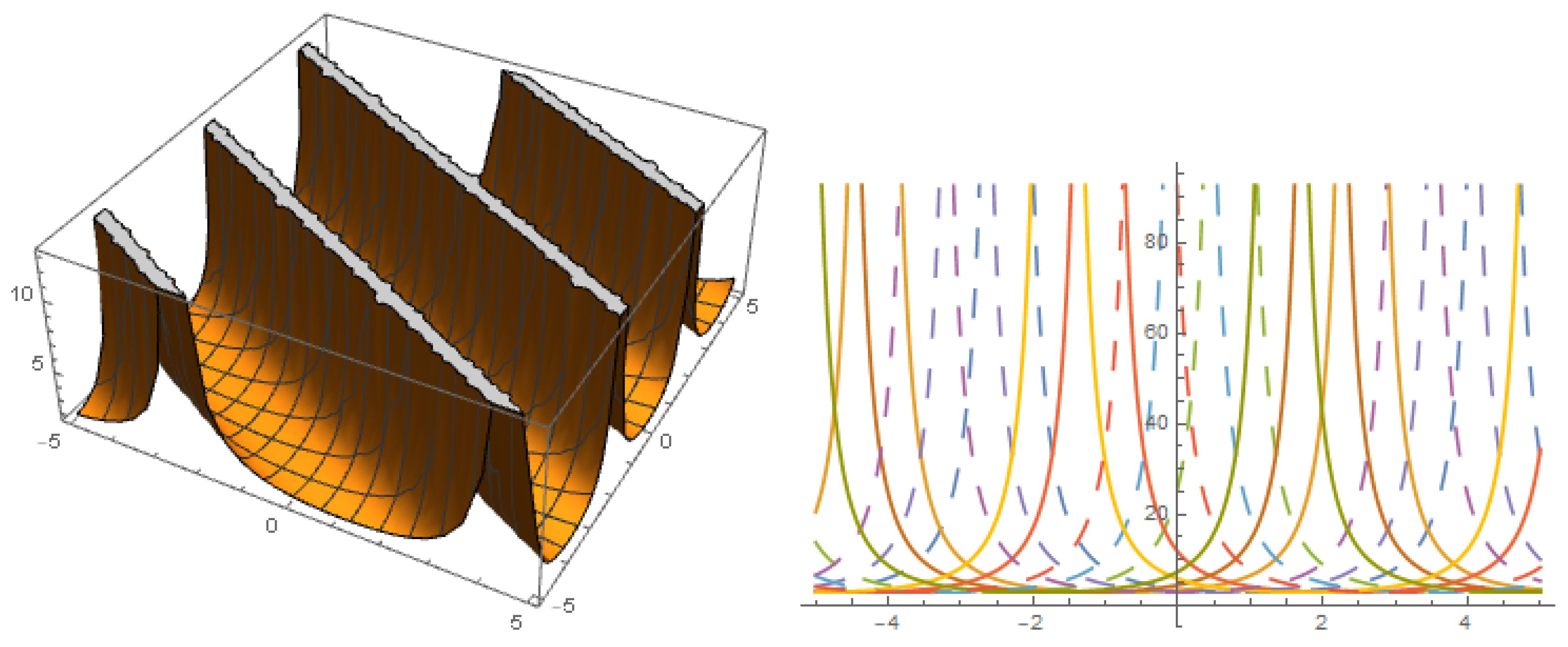
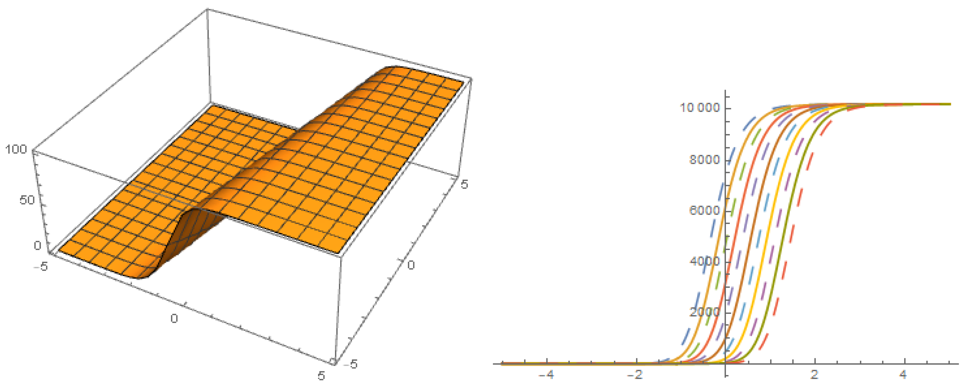
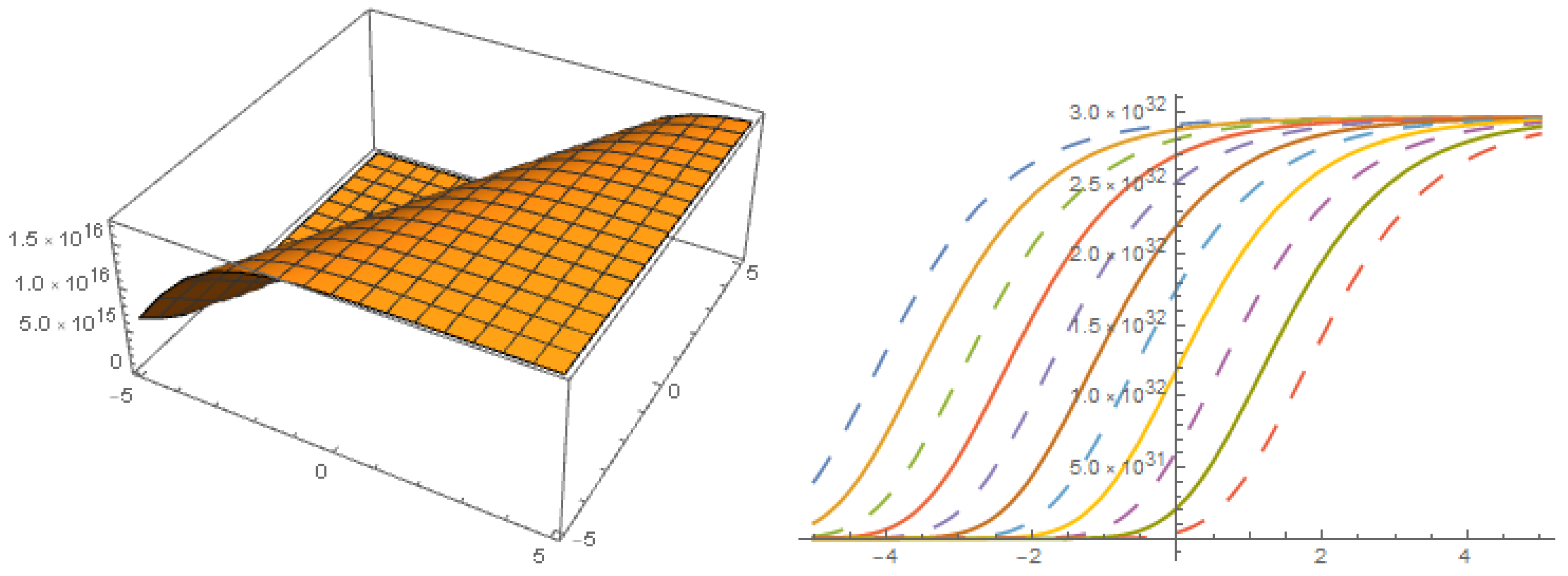
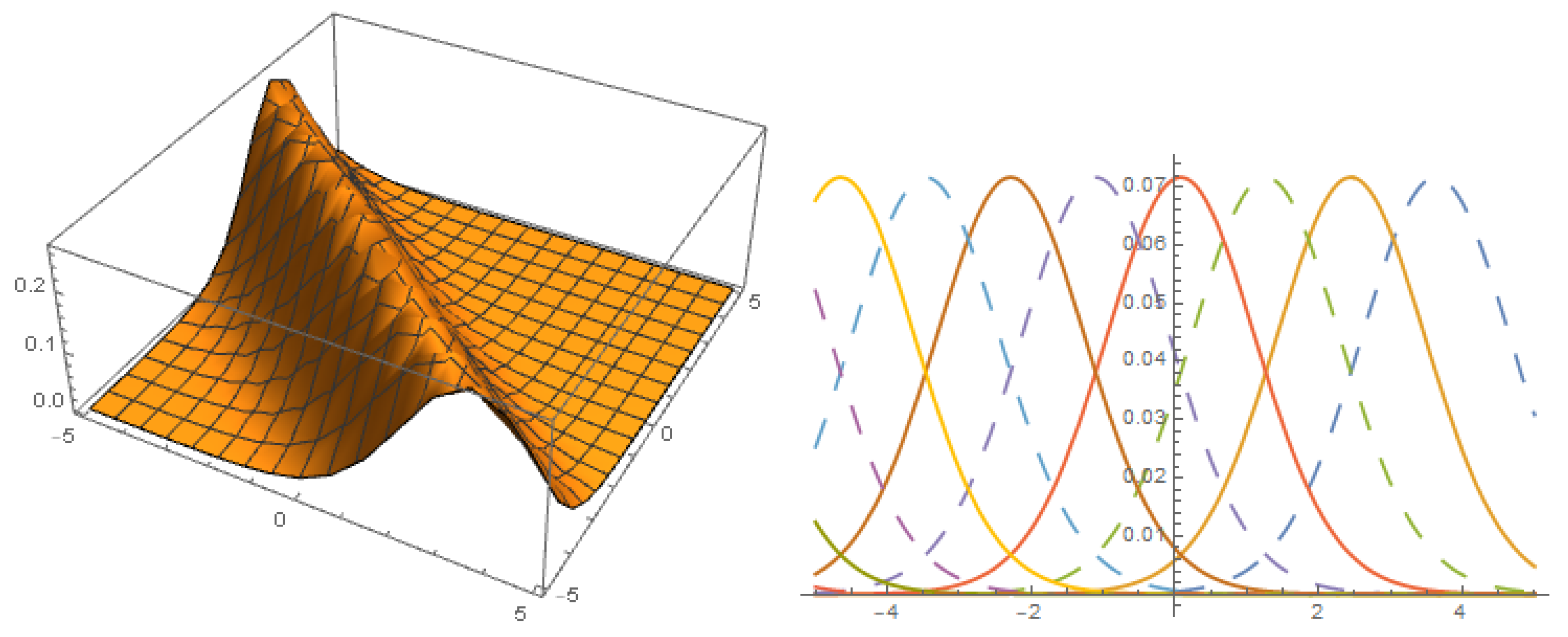
4.1. Application of Modified Extended Auxiliary Equation Mapping Method

Let solution of (76) is,
V = A 2 Ψ 2 + A 1 Ψ + A 0 + B 1 Ψ + B 2 Ψ 2 + C 2 Ψ + D 2 Ψ Ψ 2 + D 1 Ψ Ψ .
Put (77) with (5) in (76),
A 0 = β 1 D 2 , A 1 = 1 4 β 2 4 D 2 + k 1 2 + k 2 2 + k 3 2 , A 2 = 1 2 β 3 2 D 2 + k 1 2 + k 2 2 + k 3 2 , C 2 = 1 2 β 3 k 1 2 + k 2 2 + k 3 2 , D 1 = 0 , B 1 = 0 , B 2 = 0 , ω = 1 4 β 1 k 1 3 + β 1 k 2 2 k 1 + β 1 k 3 2 k 1 4 k 1 μ .
Subsitute (78) in (77),
CASE I:
V 1 = β 1 D 2 β 2 4 D 2 + k 1 2 + k 2 2 + k 3 2 β 1 ϵ coth 1 2 β 1 ξ + ξ 0 + 1 4 β 2 1 2 β 3 2 D 2 + k 1 2 + k 2 2 + k 3 2 β 1 ϵ coth 1 2 β 1 ξ + ξ 0 + 1 β 2 2 + 1 2 β 3 k 1 2 + k 2 2 + k 3 2 β 1 3 / 2 ϵ csc h 2 1 2 β 1 ξ + ξ 0 2 β 2 + D 2 β 1 3 / 2 ϵ csc h 2 1 2 β 1 ξ + ξ 0 2 β 2 β 1 ϵ coth 1 2 β 1 ξ + ξ 0 + 1 β 2 2 , β 1 > 0 , β 2 2 4 β 1 β 3 = 0 .
From (75), the solution of (79) can be written as,
U 22 = V 1 2 , β 1 > 0 , β 2 2 4 β 1 β 3 = 0 .
CASE II:
V 2 = β 1 D 2 1 4 β 2 4 D 2 + k 1 2 + k 2 2 + k 3 2 β 1 4 β 3 ϵ sinh β 1 ξ + ξ 0 cosh β 1 ξ + ξ 0 + η + 1 1 2 β 3 2 D 2 + k 1 2 + k 2 2 + k 3 2 β 1 4 β 3 ϵ sinh β 1 ξ + ξ 0 cosh β 1 ξ + ξ 0 + η + 1 2 + 1 2 β 3 k 1 2 + k 2 2 + k 3 2 1 2 β 1 β 3 β 1 ϵ cosh β 1 ξ + ξ 0 cosh β 1 ξ + ξ 0 + η β 1 ϵ sinh 2 β 1 ξ + ξ 0 cosh β 1 ξ + ξ 0 + η 2 + D 2 β 1 β 3 β 1 ϵ cosh β 1 ξ + ξ 0 cosh β 1 ξ + ξ 0 + η β 1 ϵ sinh 2 β 1 ξ + ξ 0 cosh β 1 ξ + ξ 0 + η 2 2 β 1 4 β 3 ϵ sinh β 1 ξ + ξ 0 cosh β 1 ξ + ξ 0 + η + 1 2 , β 1 > 0 , β 3 > 0 , β 2 = 4 β 1 β 3 1 / 2 .
U 23 = V 2 2 , β 1 > 0 , β 3 > 0 , β 2 = 4 β 1 β 3 1 / 2 .
CASE III:
V 3 = β 1 D 2 β 2 4 D 2 + k 1 2 + k 2 2 + k 3 2 β 1 ϵ sinh β 1 ξ + ξ 0 + P cosh β 1 ξ + ξ 0 + η P 2 + 1 + 1 4 β 2 1 2 β 3 2 D 2 + k 1 2 + k 2 2 + k 3 2 β 1 ϵ sinh β 1 ξ + ξ 0 + P cosh β 1 ξ + ξ 0 + η P 2 + 1 + 1 β 2 2 + 1 2 β 3 k 1 2 + k 2 2 + k 3 2 β 1 β 1 ϵ cosh β 1 ξ + ξ 0 cosh β 1 ξ + ξ 0 + η P 2 + 1 β 1 ϵ sinh β 1 ξ + ξ 0 sinh β 1 ξ + ξ 0 + P cosh β 1 ξ + ξ 0 + η P 2 + 1 2 β 2 + D 2 β 1 β 1 ϵ cosh β 1 ξ + ξ 0 cosh β 1 ξ + ξ 0 + η P 2 + 1 β 1 ϵ sinh β 1 ξ + ξ 0 sinh β 1 ξ + ξ 0 + P cosh β 1 ξ + ξ 0 + η P 2 + 1 2 β 2 β 1 ϵ sinh β 1 ξ + ξ 0 + P cosh β 1 ξ + ξ 0 + η P 2 + 1 + 1 β 2 2 , β 1 > 0 .
U 24 = V 3 2 , β 1 > 0 , β 3 > 0 , β 2 = 4 β 1 β 3 1 / 2 .
Figure 7. Solution U 24 with β 1 = 2 , β 2 = 0.001 , β 3 = 2 , D 2 = 3.01 , η = 1 , ξ 0 = 0.4 , k 1 = 0.7 , k 2 = 0.0001 , k 3 = 1.3 , μ = 0.5 , P = 1 , y = 1 , z = 1 , ϵ = 1 .
Symmetry 15 00248 g007

4.2. Application of Extended Simple Equation Method

Let solution of (76) is
V = A 2 Ψ 2 + A 1 Ψ + A 2 Ψ 2 + A 1 Ψ + A 0 .
Put (85) with (7) in (76),
CASE 1: c 3 = 0 ,
FAMILY-I
A 0 = c 0 c 2 k 1 2 + k 2 2 + k 3 2 , A 2 = 0 , A 1 = 0 , A 2 = c 2 2 k 1 2 + k 2 2 + k 3 2 , A 1 = c 1 c 2 k 1 2 + k 2 2 + k 3 2 , ω = 1 4 k 1 c 1 2 4 c 0 c 2 k 1 2 + k 2 2 + k 3 2 4 μ .
Put (86) in (85),
V 4 = c 0 c 2 k 1 2 + k 2 2 + k 3 2 + c 1 c 2 k 1 2 + k 2 2 + k 3 2 c 1 4 c 2 c 0 c 1 2 tan 1 2 4 c 2 c 0 c 1 2 ξ + ξ 0 2 c 2 c 2 2 k 1 2 + k 2 2 + k 3 2 c 1 4 c 2 c 0 c 1 2 tan 1 2 4 c 2 c 0 c 1 2 ξ + ξ 0 2 c 2 2 , 4 c 0 c 2 > c 1 2 .
U 25 = V 4 2 , 4 c 0 c 2 > c 1 2 .
FAMILY-II
A 0 = c 0 c 2 k 1 2 + k 2 2 + k 3 2 , A 2 = c 0 2 k 1 2 + k 2 2 + k 3 2 , A 1 = c 0 c 1 k 1 2 + k 2 2 + k 3 2 , A 2 = 0 , A 1 = 0 , ω = 1 4 k 1 c 1 2 4 c 0 c 2 k 1 2 + k 2 2 + k 3 2 4 μ .
Substitute (89) in (85),
V 5 = 4 c 2 2 c 1 4 c 2 c 0 c 1 2 tan 1 2 4 c 2 c 0 c 1 2 ξ + ξ 0 2 c 0 2 k 1 2 + k 2 2 + k 3 2 c 0 c 1 k 1 2 + k 2 2 + k 3 2 2 c 2 c 1 4 c 2 c 0 c 1 2 tan 1 2 4 c 2 c 0 c 1 2 ξ + ξ 0 c 0 c 2 k 1 2 + k 2 2 + k 3 2 , 4 c 0 c 2 > c 1 2 .
U 26 = V 5 2 , 4 c 0 c 2 > c 1 2 .
CASE 2: c 0 = 0 , c 3 = 0 ,
A 0 = 0 , A 2 = 0 , A 1 = 0 , A 2 = c 2 2 k 1 2 + k 2 2 + k 3 2 , A 1 = c 1 c 2 k 1 2 + k 2 2 + k 3 2 , ω = 1 4 c 1 2 k 1 3 + c 1 2 k 2 2 k 1 + c 1 2 k 3 2 k 1 4 k 1 μ .
Put (92) in (85),
V 6 = c 1 c 2 k 1 2 + k 2 2 + k 3 2 c 1 exp c 1 ξ + ξ 0 1 c 2 exp c 1 ξ + ξ 0 c 2 2 k 1 2 + k 2 2 + k 3 2 c 1 exp c 1 ξ + ξ 0 1 c 2 exp c 1 ξ + ξ 0 2 , c 1 > 0 ,
U 27 = V 6 2 , c 1 > 0 .
V 7 = c 2 2 k 1 2 + k 2 2 + k 3 2 c 1 exp c 1 ξ + ξ 0 c 2 exp c 1 ξ + ξ 0 + 1 2 c 1 c 2 k 1 2 + k 2 2 + k 3 2 c 1 exp c 1 ξ + ξ 0 c 2 exp c 1 ξ + ξ 0 + 1 , c 1 < 0 .
U 28 = V 6 2 , c 1 < 0 .
CASE 3: c 1 = 0 , c 3 = 0 ,
FAMILY-I
A 0 = c 0 c 2 k 1 2 + k 2 2 + k 3 2 , A 2 = 0 , A 1 = 0 , A 2 = c 2 2 k 1 2 + k 2 2 + k 3 2 , A 1 = 0 , ω = k 1 c 0 c 2 k 1 2 + c 0 c 2 k 2 2 + c 0 c 2 k 3 2 + μ .
Put (97) in (85),
V 8 = c 2 2 k 1 2 + k 2 2 + k 3 2 c 0 c 2 tan c 0 c 2 ξ + ξ 0 c 2 2 c 0 c 2 k 1 2 + k 2 2 + k 3 2 , c 0 c 2 > 0 ,
U 29 = V 8 2 , c 0 c 2 > 0 .
V 9 = c 2 2 k 1 2 + k 2 2 + k 3 2 c 0 c 2 tanh c 0 c 2 ξ + ξ 0 c 2 2 c 0 c 2 k 1 2 + k 2 2 + k 3 2 , c 0 c 2 < 0 .
U 30 = V 9 2 , c 0 c 2 < 0 .
Figure 8. Solution U 26 with c 0 = 0.05 , c 1 = 1.07 , c 2 = 1 , D 2 = 3.01 , ξ 0 = 0.4 , k 1 = 0.7 , k 2 = 0.1 , k 3 = 1.3 , μ = 1.7 , y = 1 , z = 1 .
Symmetry 15 00248 g008
FAMILY-II
A 0 = c 0 c 2 k 1 2 + k 2 2 + k 3 2 , A 2 = c 0 2 k 1 2 + k 2 2 + k 3 2 , A 1 = 0 , A 2 = 0 , A 1 = 0 , ω = k 1 c 0 c 2 k 1 2 + c 0 c 2 k 2 2 + c 0 c 2 k 3 2 + μ .
Put (102) in (85),
V 10 = c 0 2 k 1 2 + k 2 2 + k 3 2 c 0 c 2 tan c 0 c 2 ξ + ξ 0 c 2 2 c 2 c 0 k 1 2 + k 2 2 + k 3 2 , c 0 c 2 > 0 ,
U 31 = V 10 2 , c 0 c 2 > 0 , .
V 11 = c 0 2 k 1 2 + k 2 2 + k 3 2 c 0 c 2 tanh c 0 c 2 ξ + ξ 0 c 2 2 c 2 c 0 k 1 2 + k 2 2 + k 3 2 , c 0 c 2 < 0 .
U 32 = V 11 2 , c 0 c 2 < 0 .
FAMILY-III
A 0 = 2 c 0 c 2 k 1 2 + k 2 2 + k 3 2 , A 2 = c 0 2 k 1 2 + k 2 2 + k 3 2 , A 1 = 0 , A 2 = c 2 2 k 1 2 + k 2 2 + k 3 2 , A 1 = 0 , ω = 4 c 0 c 2 k 1 3 4 c 0 c 2 k 2 2 k 1 4 c 0 c 2 k 3 2 k 1 k 1 μ .
Put (107) in (85),
V 12 = c 2 2 k 1 2 + k 2 2 + k 3 2 c 0 c 2 tan c 0 c 2 ξ + ξ 0 c 2 2 c 0 2 k 1 2 + k 2 2 + k 3 2 c 0 c 2 tan c 0 c 2 ξ + ξ 0 c 2 2 2 c 2 c 0 k 1 2 + k 2 2 + k 3 2 , c 0 c 2 > 0 ,
U 33 = V 12 2 , c 0 c 2 > 0 ,
V 13 = c 2 2 k 1 2 + k 2 2 + k 3 2 c 0 c 2 tanh c 0 c 2 ξ + ξ 0 c 2 2 c 0 2 k 1 2 + k 2 2 + k 3 2 c 0 c 2 tanh c 0 c 2 ξ + ξ 0 c 2 2 2 c 2 c 0 k 1 2 + k 2 2 + k 3 2 , c 0 c 2 < 0 .
U 34 = V 13 2 , c 0 c 2 < 0 . ,

4.3. Application of Modified F-Expansion Method

Let (76) has solution,
V = a 2 F 2 + a 1 F + a 0 + b 2 F 2 + b 1 F .
Put (112) with (9) in (76).
A = 0, B = 1, C = −1,
a 0 = 0 , a 2 = k 1 2 k 2 2 k 3 2 , a 1 = k 1 2 + k 2 2 + k 3 2 , b 1 = 0 , b 2 = 0 , ω = 1 4 4 k 1 μ + k 1 3 + k 2 2 k 1 + k 3 2 k 1 .
Put (113) in (112),
V 14 = k 3 2 1 2 tanh ξ 2 + 1 2 + k 1 2 + k 2 2 + ( k 1 2 k 2 2 k 3 2 ) 1 2 tanh ξ 2 + 1 2 2 .
U 35 = V 14 2 .
A = 0, C = 1, B = −1,
a 0 = 0 , a 2 = k 1 2 + k 2 2 + k 3 2 , a 1 = k 1 2 + k 2 2 + k 3 2 , b 1 = 0 , b 2 = 0 , ω = 1 4 4 k 1 μ + k 1 3 + k 2 2 k 1 + k 3 2 k 1 .
Put (116) into (112),
V 15 = k 3 2 1 2 1 2 coth ξ 2 + k 1 2 + k 2 2 + k 1 2 + k 2 2 + k 3 2 1 2 1 2 coth ξ 2 2 .
U 36 = V 15 2 .
A = 1/2, B = 0, C = −1/2
a 0 = 1 4 k 1 2 + k 2 2 + k 3 2 , a 2 = 0 , a 1 = 0 , b 1 = 0 , b 2 = 1 4 k 1 2 k 2 2 k 3 2 , ω = 1 4 4 k 1 μ + k 1 3 + k 2 2 k 1 + k 3 2 k 1 .
Substitute (119) into (112),
V 16 = 1 4 k 1 2 k 2 2 k 3 2 1 ( cot ( ξ ) + csc ( ξ ) ) 2 .
U 37 = V 16 2 .
A = 1, B = 0, C = −1
a 0 = k 1 2 + k 2 2 + k 3 2 , a 2 = 0 , a 1 = 0 , b 1 = 0 , b 2 = k 1 2 k 2 2 k 3 2 , ω = k 1 μ + k 1 3 + k 2 2 k 1 + k 3 2 k 1 .
Put (122) in (112),
V 17 = k 1 2 k 2 2 k 3 2 1 tanh 2 ( ξ ) .
U 38 = V 17 2 .
A = C = 1/2, B = 0,
a 0 = 1 4 k 1 2 k 2 2 k 3 2 , a 2 = 0 , a 1 = 0 , b 1 = 0 , b 2 = 1 4 k 1 2 k 2 2 k 3 2 , ω = 1 4 k 1 k 1 2 + k 2 2 + k 3 2 + 4 μ .
Put (125) in (112),
V 18 = 1 4 k 1 2 k 2 2 k 3 2 + 1 4 k 1 2 k 2 2 k 3 2 1 ( tan ( ξ ) + sec ( ξ ) ) 2 .
U 39 = V 18 2 .
A = C = −1/2, B = 0,
a 0 = 1 4 k 1 2 k 2 2 k 3 2 , a 2 = 0 , a 1 = 0 , b 1 = 0 , b 2 = 1 4 k 1 2 k 2 2 k 3 2 , ω = 1 4 k 1 k 1 2 + k 2 2 + k 3 2 + 4 μ .
Put (128) in (112),
V 19 = 1 4 k 1 2 k 2 2 k 3 2 + 1 4 k 1 2 k 2 2 k 3 2 1 ( sec ( ξ ) tan ( ξ ) ) 2 .
U 40 = V 19 2 .
A = C = −1, B = 0,
a 0 = k 1 2 k 2 2 k 3 2 , a 2 = 0 , a 1 = 0 , b 1 = 0 , b 2 = k 1 2 k 2 2 k 3 2 , ω = k 1 k 1 2 + k 2 2 + k 3 2 + μ .
Put (131) in (112),
V 20 = k 1 2 k 2 2 k 3 2 + k 1 2 + k 2 2 + k 3 2 ) 1 tan 2 ( ξ ) .
U 41 = V 20 2 .
Figure 9. Solution U 29 with c 0 = 1.3 , c 2 = 0.1 , D 2 = 0.01 , λ = 0.4 , k 1 = 1.4 , k 2 = 1.1 , k 3 = 0.1 , μ = 0.03 , y = 1 , z = 1 .
Symmetry 15 00248 g009
Figure 10. Solution U 35 with D 2 = 0.1 , k 1 = 1.03 , k 2 = 1.1 , k 3 = 0.1 , μ = 0.3 , y = 1 , z = 1 .
Symmetry 15 00248 g010
A = B = 0
a 0 = 0 , a 2 = C 2 k 1 2 + k 2 2 + k 3 2 , a 1 = 0 , b 1 = 0 , b 2 = 0 , ω = k 1 ( μ ) .
Put (134) in (112),
V 21 = C 2 k 1 2 + k 2 2 + k 3 2 1 C ξ + η 2 .
U 42 = V 21 2 .
B = C = 0
a 0 = 0 , a 2 = 0 , a 1 = 0 , b 1 = 0 , b 2 = A 2 k 1 2 + k 2 2 + k 3 2 , ω = k 1 ( μ ) .
Put (137) in (112),
V 22 = A 2 k 1 2 + k 2 2 + k 3 2 1 1 A ξ 2 .
U 43 = V 22 2 .
C = 0
a 0 = 0 , a 2 = 0 , a 1 = 0 , b 1 = A B k 1 2 + k 2 2 + k 3 2 , b 2 = A 2 k 1 2 + k 2 2 + k 3 2 , ω = 1 4 k 1 B 2 k 1 2 + B 2 k 2 2 + B 2 k 3 2 4 . μ
Put (140) in (112),
V 23 = A B k 1 2 + k 2 2 + k 3 2 1 B e B ξ A A 2 k 1 2 + k 2 2 + k 3 2 1 B e B ξ A 2 .
U 44 = V 23 2 .
Figure 11. Solution U 40 with D 2 = 2.1 , k 1 = 1.03 , k 2 = 1.1 , k 3 = 2.1 , μ = 3.3 , y = 1 , z = 1 .
Symmetry 15 00248 g011

5. Conclusions

Three mathematical schemes have employed to investigate solutions of NLEQZ and NLmQZK models. The derived solutions are in diverse types like exponential, hyperbolic, trigonometric and rational functions. Some solutions are plotted graphically in 2-dimensional and 3-dimensional by imparting particular value to the parameters under the constrain condition on each disquiet solution. Hence, it shows that our proposed mathematical methods are powerful, melodious and capacity be used in supplementary works to originate novel results for NPDEs ascending in physical science.

Author Contributions

Conceptualization, M.A., A.R.S., A.A., A.F.A. (Abdulrahman F. AlJohani), W.A. and A.F.A. (Amal F. Alharbi); methodology, M.A., A.R.S., A.A., A.F.A. (Abdulrahman F. AlJohani), W.A. and A.F.A. (Amal F. Alharbi); software, M.A., A.R.S., A.A., A.F.A. (Abdulrahman F. AlJohani), W.A. and A.F.A. (Amal F. Alharbi); validation, M.A., A.R.S., A.A., A.F.A. (Abdulrahman F. AlJohani), W.A. and A.F.A. (Amal F. Alharbi); formal analysis, M.A., A.R.S., A.A., A.F.A. (Abdulrahman F. AlJohani), W.A. and A.F.A. (Amal F. Alharbi); investigation, M.A., A.R.S., A.A., A.F.A. (Abdulrahman F. AlJohani), W.A. and A.F.A. (Amal F. Alharbi); resources, M.A., A.R.S., A.A., A.F.A. (Abdulrahman F. AlJohani), W.A. and A.F.A. (Amal F. Alharbi); data curation, M.A., A.R.S., A.A., A.F.A. (Abdulrahman F. AlJohani), W.A. and A.F.A. (Amal F. Alharbi); writing—original draft preparation, M.A., A.R.S., A.A., A.F.A. (Abdulrahman F. AlJohani), W.A. and A.F.A. (Amal F. Alharbi); writing—review and editing, M.A., A.R.S., A.A., A.F.A. (Abdulrahman F. AlJohani), W.A. and A.F.A. (Amal F. Alharbi); visualization, M.A., A.R.S., A.A., A.F.A. (Abdulrahman F. AlJohani), W.A. and A.F.A. (Amal F. Alharbi). All authors have read and agreed to the published version of the manuscript.

Funding

Deanship of Scientific Research (DSR), University of Tabuk, Tabuk, Saudi Arabia.

Data Availability Statement

Not applicable.

Acknowledgments

The authors would like to acknowledge support for this work from the Scientific Research (DSR), University of Tabuk, Tabuk, Saudi Arabia, under Grant no. S-1442-0159.

Conflicts of Interest

The authors declare no conflict of interest.

References

  1. Islam, M.N.; Asaduzzaman, M.; Ali, M.S. Exact wave solutions to the simplified modified Camassa-Holm equation in mathematical physics. AIMS Math. 2020, 5, 26–41. [Google Scholar] [CrossRef]
  2. Asaduzzaman, M.; Ali, M.Z. Existence of multiple positive solutions to the Caputo-type nonlinear fractional Differential equation with integral boundary value conditions. Fixed Point Theory 2022, 23, 127–142. [Google Scholar] [CrossRef]
  3. Gharami, P.P.; Gazi, M.A.; Ananna, S.N.; Ahmmed, S.F. Numerical exploration of MHD unsteady flow of THNF passing through a moving cylinder with Soret and Dufour effects. Partial. Differ. Equ. Appl. Math. 2022, 6, 100463. [Google Scholar] [CrossRef]
  4. Ananna, S.N.; Gharami, P.P.; An, T.; Asaduzzaman, M. The improved modified extended tanh-function method to develop the exact travelling wave solutions of a family of 3D fractional WBBM equations. Results Phys. 2022, 41, 105969. [Google Scholar]
  5. Rozenman, G.G.; Shemer, L.; Arie, A. Observation of accelerating solitary wavepackets. Phys. Rev. E 2020, 101, 050201. [Google Scholar] [CrossRef] [PubMed]
  6. Al-Ghafri, K.S.; Krishnan, E.V.; Khan, S.; Biswas, A. Optical Bullets and Their Modulational Instability Analysis. Appl. Sci. 2022, 12, 9221. [Google Scholar] [CrossRef]
  7. Houwe, A.; Inc, M.; Doka, S.Y.; Akinlar, M.A.; Baleanu, D. Chirped solitons in negative index materials generated by Kerr nonlinearity. Results Phys. 2020, 17, 103097. [Google Scholar] [CrossRef]
  8. Kudryashov, N.A. One method for finding exact solutions of nonlinear differential equations. Commun. Nonlinear Sci. Numer. Simul. 2012, 17, 2248. [Google Scholar] [CrossRef] [Green Version]
  9. Zayed, E.M.E.; Arnous, A.H. DNA dynamics studied using the homogeneous balance method. Chin. Phys. Lett. 2012, 29, 080203. [Google Scholar] [CrossRef]
  10. Houwe, A.; Abbagari, S.; Salathiel, Y.; Inc, M.; Doka, S.Y.; Crépin, K.T.; Doka, S.Y. Complex traveling-wave and solitons solutions to the Klein-Gordon-Zakharov equations. Results Phys. 2020, 17, 103127. [Google Scholar] [CrossRef]
  11. Kudryashov, N.A.; Ryabov, P.N.; Fedyanin, T.E.; Kutukov, A.A. Evolution of pattern formation under ion bombardment of substrate. Phys. Lett. A 2013, 377, 753–759. [Google Scholar] [CrossRef]
  12. Kudryashov, N.A. Polynomials in logistic function and solitary waves of nonlinear differential equations. Appl. Math. Comput. 2013, 219, 9245–9253. [Google Scholar] [CrossRef]
  13. Ryabov, P.N.; Sinelshchikov, D.I.; Kochanov, M.B. Application of the Kudryashov method for finding exact solutions of the high order nonlinear evolution equations. Appl. Math. Comput. 2011, 218, 3965–3972. [Google Scholar] [CrossRef] [Green Version]
  14. Houwe, A.; Abbagari, S.; Inc, M.; Betchewe, G.; Doka, S.Y.; Crépin, K.T. Chirped solitons in discrete electrical transmission line. Results Phys. 2020, 18, 103188. [Google Scholar] [CrossRef]
  15. Wang, M.; Li, X.; Zhang, J. The (G’ G)-expansion method and travelling wave solutions of nonlinear evolution equations in mathematical physics. Phys. Lett. A 2008, 372, 417–423. [Google Scholar] [CrossRef]
  16. Ismail, A.; Turgut, O. Analytic study on two nonlinear evolution equations by using the (G’/G)-expansion method. Appl. Math. Comput. 2009, 209, 425–429. [Google Scholar]
  17. Nestor, S.; Nestor, G.B.; Inc, M.; Doka, S.Y. Exact traveling wave solutions to the higher-order nonlinear Schrödinger equation having Kerr nonlinearity form using two strategic integrations. Eur. Phys. J. Plus 2020, 135, 380. [Google Scholar] [CrossRef]
  18. Nestor, S.; Abbagari, S.; Houwe, A.; Inc, M.; Betchewe, G.; Doka, S.Y. Diverse chirped optical solitons and new complex traveling waves in nonlinear optical fibers. Commun. Theor. Phys. 2020, 72, 065501. [Google Scholar] [CrossRef]
  19. Nestor, S.; Houwe, A.; Rezazadeh, H.; Bekir, A.; Betchewe, G.; Doka, S.Y. New solitary waves for the Klein-Gordon-Zakharov equations. Mod. Phys. Lett. B 2020, 34, 2050246. [Google Scholar] [CrossRef]
  20. Nestor, S.; Houwe, A.; Betchewe, G.; Inc, M.; Doka, S.Y. A series of abundant new optical solitons to the conformable space-time fractional perturbed nonlinear Schrödinger equation. Phys. Scr. 2020, 95, 085108. [Google Scholar] [CrossRef]
  21. Nestor, S.; Betchewe, G.; Rezazadeh, H.; Bekir, A.; Doka, S.Y. Exact optical solitons to the perturbed nonlinear Schrödinger equation with dual-power law of nonlinearity. Opt. Quantum Electron. 2020, 52, 318. [Google Scholar]
  22. Abbagari, S.; Korkmaz, A.; Rezazadeh, H.; Mukam, S.P.T.; Bekir, A. Soliton solutions in different classes for the Kaup–Newell model equation. Mod. Phys. Lett. B 2020, 34, 2050038. [Google Scholar]
  23. Abbagari, S.; Ali, K.K.; Rezazadeh, H.; Eslami, M.; Mirzazadeh, M.; Korkmaz, A. The propagation of waves in thin-film ferroelectric materials. Pramana J. Phys. 2019, 93, 27. [Google Scholar]
  24. Abbagari, S.; Kuetche, V.K.; Bouetou, T.B.; Kofane, T.C. Scattering behavior of waveguide channels of a new coupled integrable dispersionless system. Chin. Phys. Lett. 2011, 28, 120501. [Google Scholar]
  25. Abbagari, S.; Kuetche, V.K.; Bouetou, T.B.; Kofane, T.C. Traveling wave-guide channels of a new coupled integrable dispersionless system. Commun. Theor. Phys. 2012, 57, 10. [Google Scholar]
  26. Abbagari, S.; Youssoufa, S.; Tchokouansi, H.T.; Kuetche, V.K.; Bouetou, T.B.; Kofane, T.C. N-rotating loop-soliton solution of the coupled integrable dispersionless equation. J. Appl. Math. Phys. 2017, 5, 1370–1379. [Google Scholar] [CrossRef] [Green Version]
  27. Mukam, S.P.T.; Abbagari, S.; Kuetche, V.K.; Bouetou, T.B. Generalized Darboux transformation and parameter-dependent rogue wave solutions to a nonlinear Schrödinger system. Nonlinear Dyn. 2018, 93, 56. [Google Scholar] [CrossRef]
  28. Yepez-Martinez, H.; Rezazadeh, H.; Abbagari, S.; Mukam, S.P.T.; Eslami, M.; Kuetche, V.K.; Bekir, A. The extended modified method applied to optical solitons solutions in birefringent fibers with weak nonlocal nonlinearity and four wave mixing. Chin. J. Phys. 2019, 58, 137–150. [Google Scholar] [CrossRef]
  29. Mukam, S.P.T.; Abbagari, S.; Kuetche, V.K.; Bouetou, T.B. Rogue wave dynamics in barotropic relaxing media. Pramana. Pramana J. Phys. 2018, 91, 56. [Google Scholar] [CrossRef]
  30. Inc, M.; Rezazadeh, H.; Baleanu, D. New solitary wave solutions for variants of (3 + 1)-dimensional Wazwaz-Benjamin-Bona-Mahony equations. Front. Phys. 2020, 8, 332. [Google Scholar]
  31. Houwe, A.; Yakada, S.; Abbagari, S.; Youssoufa, S.; Inc, M.; Doka, S.Y. Survey of third-and fourth-order dispersions including ellipticity angle in birefringent fibers on W-shaped soliton solutions and modulation instability analysis. Eur. Phys. J. Plus 2021, 136, 357. [Google Scholar] [CrossRef]
  32. Wang, J.; Zhang, R.; Yang, L. New metamaterial mathematical modeling of acoustic topological insulators via tunable underwater local resonance. Appl. Math. Comput. 2020, 136, 125426. [Google Scholar]
  33. Wang, J.; Zhang, R.; Yang, L. Solitary waves of nonlinear barotropic–baroclinic coherent structures. Phys. Fluids 2020, 32, 096604. [Google Scholar] [CrossRef]
  34. Zhang, R.; Yang, L. Theoretical analysis of equatorial near-inertial solitary waves under complete Coriolis parameters. Acta Oceanol. Sin. 2021, 40, 54–61. [Google Scholar] [CrossRef]
  35. Zhang, R.; Yang, L. Nonlinear Rossby waves in zonally varying flow under generalized beta approximation. Dyn. Atmos. Oceans 2019, 85, 16–27. [Google Scholar] [CrossRef]
  36. Elsayed, M.E.Z.; Reham, M.A.S.; Abdul-Ghani, A.-N. On solving the (3+ 1)-dimensional NLEQZK equation and the (3+ 1)-dimensional NLmZK equation using the extended simplest equation method. Comput. Math. Appl. 2019, 87, 3390. [Google Scholar]
  37. El-Taibany, W.F.; El-Labany, S.K.; Behery, E.E.; Abdelghany, A.M. Nonlinear dust acoustic waves in a self-gravitating and opposite-polarity complex plasma medium. Eur. Phys. J. Plus 2019, 134, 457. [Google Scholar] [CrossRef]
  38. Sabry, R.; Moslem, W.M.; Haas, F.; Seadawy, A.R. Dust acoustic solitons in plasmas with kappa-distributed electrons and/or ions. Phys. Plasmas 2008, 15, 1. [Google Scholar]
  39. El-Shiekh, R.M.; Al-Nowehy, A.-G. Integral methods to solve the variable coefficient nonlinear Schrödinger equation. Z. Natuforsch. 2013, 68, 255–260. [Google Scholar] [CrossRef] [Green Version]
  40. Munro, S.; Parkes, E. The derivation of a modified Zakharov–Kuznetsov equation and the stability of its solutions. J. Plasma Phys. 1999, 62, 305–317. [Google Scholar] [CrossRef]
  41. Seadawy, A.R.; Ali, A.; Althobaiti, S.; El-Rashidy, K. Construction of abundant novel analytical solutions of the space–time fractional nonlinear generalized equal width model via Riemann–Liouville derivative with application of mathematical methods. Open Phys. 2021, 19, 657–668. [Google Scholar] [CrossRef]
  42. Seadawy, A.R.; Ali, A.; Helal, M.A. Analytical wave solutions of the (2+1)-dimensional Boiti–Leon–Pempinelli and Boiti–Leon–Manna–Pempinelli equations by mathematical methods. Math Meth Appl Sci. 2021, 44, 14292–14315. [Google Scholar] [CrossRef]
  43. Seadawy, A.R. Three-dimensional nonlinear modified Zakharov–Kuznetsov equation of ion-acoustic waves in a magnetized plasma. Comput. Math. Appl. 2016, 71, 201–212. [Google Scholar] [CrossRef]
Figure 1. The profile of solution U 1 with β 1 = 2 , β 2 = 4 , β 3 = 2 , β = 0.5 , γ = 4.5 , ξ 0 = 4 , P = 0.05 , Q = 2 , R = 0.1 ,   S = 2.5 , ω = 0.05 , y = 1 , z = 1 , ϵ = 1 .
Symmetry 15 00248 g001
Disclaimer/Publisher’s Note: The statements, opinions and data contained in all publications are solely those of the individual author(s) and contributor(s) and not of MDPI and/or the editor(s). MDPI and/or the editor(s) disclaim responsibility for any injury to people or property resulting from any ideas, methods, instructions or products referred to in the content.

