DOA Estimation of Indoor Sound Sources Based on Spherical Harmonic Domain Beam-Space MUSIC

Abstract

The Multiple Signal Classification (MUSIC) algorithm has become one of the most popular algorithms for estimating the direction-of-arrival (DOA) of multiple sources due to its simplicity and ease of implementation. Spherical microphone arrays can capture more sound field information than planar arrays. The collected multichannel speech signals can be transformed from the space domain to the spherical harmonic domain (SHD) for processing through spherical modal decomposition. The spherical harmonic domain MUSIC (SHD-MUSIC) algorithm reduces the dimensionality of the covariance matrix and achieves better DOA estimation performance than the conventional MUSIC algorithm. However, the SHD-MUSIC algorithm is prone to failure in low signal-to-noise ratio (SNR), high reverberation time (RT), and other multi-source environments. To address these challenges, we propose a novel joint spherical harmonic domain beam-space MUSIC (SHD-BMUSIC) algorithm in this paper. The advantage of decoupling the signal frequency and angle information in the SHD is exploited to improve the anti-reverberation property of the DOA estimation. In the SHD, the broadband beamforming matrix converts the SHD sound pressure to the beam domain output. Beamforming enhances the incoming signal in the desired direction and reduces the SNR threshold as well as the dimension of the signal covariance matrix. In addition, the 3D beam of the spherical array has rotational symmetry and its beam steering is decoupled from the beam shape. Therefore, the broadband beamforming constructed in this paper allows for the arbitrary adjustment of beam steering without the need to redesign the beam shape. Both simulation experiments and practical tests are conducted to verify that the proposed SHD-BMUSIC algorithm has a more robust adjacent source discrimination capability than the SHD-MUSIC algorithm.

1. Introduction

The ability to localize acoustic events is a fundamental prerequisite for equipping microphones with awareness of their surrounding environment. Source localization provides estimates of positional information, e.g., Directions-of-Arrival (DOAs) [1]. Conventional DOA estimation methods are mainly based on time difference of arrival (TDOA) [2], steered response power—phase transform (SRP-PHAT) [3], beam scanning [4], and spatial covariance matrix (SCM) [5]—and so on. The high-resolution spectral estimation method, such as Multiple Signal Classification (MUSIC), has received much attention because it can break the Rayleigh limit constraint and has a more promising direction resolution. However, while handling coherent sources of broadband signals in a reverberant environment, the high-resolution spectral estimation method suffers from a large spectral peak search operation, sensitivity to array error, and a high-resolution SNR threshold. These shortcomings often have a great negative impact on research, which is worth considering deeply.

In recent years, the theory of spherical microphone arrays has been widely used and developed. For DOA estimation of multiple sound sources, the spherical microphone array [6,7,8] has become a key and universal research focus. Compared with a linear and planar array, the spherical array has rotational symmetry and is easy for beamforming [9,10]. The spherical microphone array enables sampling of non-confounding sound pressure to reconstruct the 3D sound field accurately. Furthermore, the sound pressure received can be transformed into the spherical harmonic domain (SHD) for processing [11]. Using the spherical Fourier transform (SFT), the spherical sound pressure received can be decomposed into several orders of spherical harmonic function combinations [12]. Thus, a MUSIC and Root-MUSIC pseudo-spectrum can be constructed in the SHD [13]. This spherical wave decomposition can separate the frequency and angular components of the sound source from each other. In [14], the authors used the frequency smoothing method to de-correlate the coherent sources, which improved the estimation performance of the SHD-MUSIC algorithm in the presence of coherent sources. However, it is clear that the signal subspace turns out not absolutely orthogonal to the noise subspace in the sound field environments. As a result, the SHD-MUSIC algorithm is sensitive to the effect of noise. There is a phenomenon called the subspace swap. The data covariance matrix cannot always hold at full-rank, which affects the correctness of the matrix decomposition results. The above reasons eventually reduce the performance of the DOA estimation algorithm in case of low SNRs. In the open spherical arrays [15], the zero point of the spherical Bessel function causes a low value of the spherical mode amplitude response [16]. At the Bessel zero points, the low amplitude problem of spherical modal amplitude cannot be responded to perfectly, so the direction of the signal source cannot be estimated. Two ideas can solve the Bessel zero problem: spherical configuration and algorithmic optimization. For example, we can use directional microphone arrays, rigid-sphere arrays [17], and dual-sphere arrays [18] under these circumstances. In [19], the authors proposed the SHD-RMUSIC algorithm using relative sound pressure values that are insensitive to noise to improve the robustness to noise. However, the algorithm could not achieve satisfactory performance at lower SNRs (below 5 dB) and was not applicable to strong reverberation (above 0.6 s) environments. To improve the performance of source direction estimation in strongly reverberant environments, the authors proposed the direct path dominance test (DPD-MUSIC) [20]. The DPD algorithm exploits the non-smoothness and sparsity of the speech signal. By selecting time-frequency bins (TF-bins) that contain the direct sound dominance of a target source without the remaining reflected sound contribution, these TF-bins are used to construct the spatial spectrum. Thus, a certain reverberation multi-path distortion problem is solved in some scenarios, and multiple sources can be localized in a 3D strongly reverberant environment. However, its application presupposes that most of the TF-bins candidate sets must contain correct DOA information and that the proportion of TF-bins containing correct DOA information is sufficient to estimate the sound source DOA reliably. To make this application prerequisite guaranteed, the authors proposed an improved DPD test method, called the DPD-EDS test [21]. The test identifies the TF-bins dominated by the direct sound by means of enhanced decomposition based on the direct sound. This improves the accuracy of selecting the TF-bins that contain the correct DOA information. Obviously, the DPD test requires a direct acoustic prior [22], which is often difficult to obtain in harsh sound field environments. This shows that the rigid spherical microphone arrays for indoor DOA estimation of multiple adjacent sources to attenuate the effects of low-SNR environments and Bessel zeros on DOA estimation performance are an effective avenue of research.

In this paper, a rigid spherical microphone array is used to perform DOA estimation of indoor sound sources by placing 32 omnidirectional microphones in a uniform sampling distribution on the surface of a rigid baffle. We propose a joint SHD-beamforming and beam-domain MUSIC algorithm solution. It is promising and profound that the proposed method can improve the resolution probability of adjacent sound sources and reduce the SNR resolution thresholds. In a nutshell, our contributions are the following:

• We propose a novel spherical harmonic domain beam-space MUSIC algorithm. Combined with the advantages of the rigid-sphere configuration, the effects of the low SNR environment and Bessel’s zero on the performance of multi-source DOA estimation are better reduced. This results in a more robust multi-source localization capability and adjacent source discrimination;
• We use a quadratic-constraint quadratic-planning optimization method to generate a multi-objective optimized signal-independent beam weight. We construct a very flexible rotationally symmetric beamformer so that the 3D beam of the spherical array can be arbitrarily redirected without redesigning the beam shape;
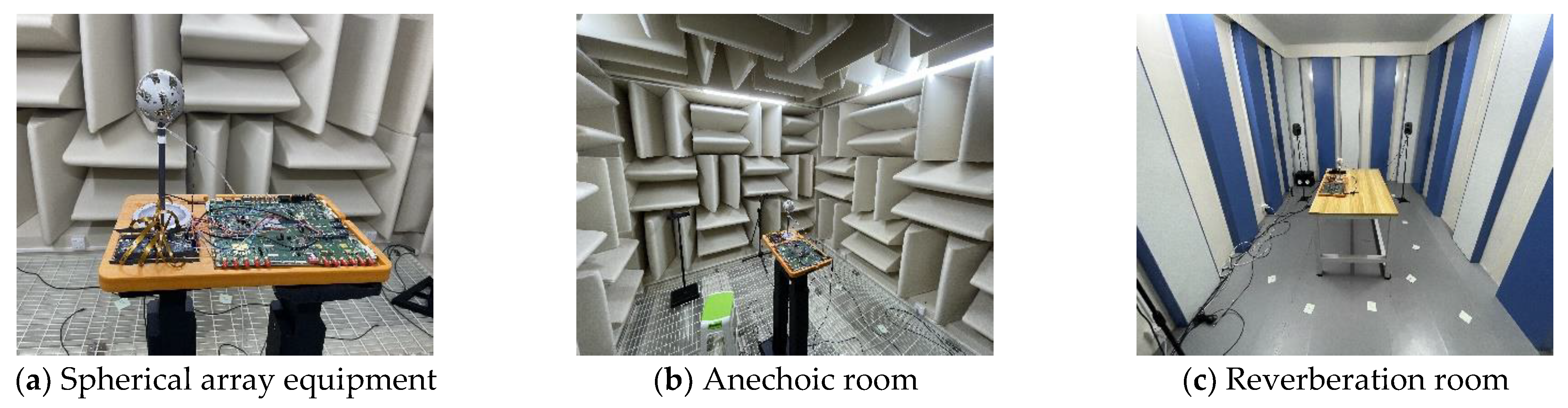
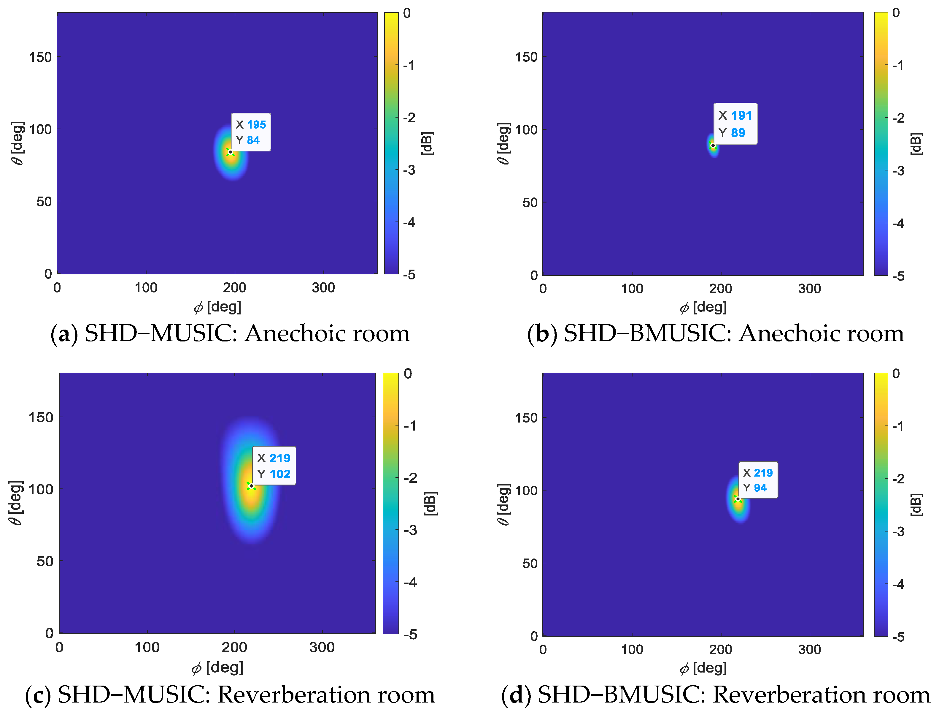
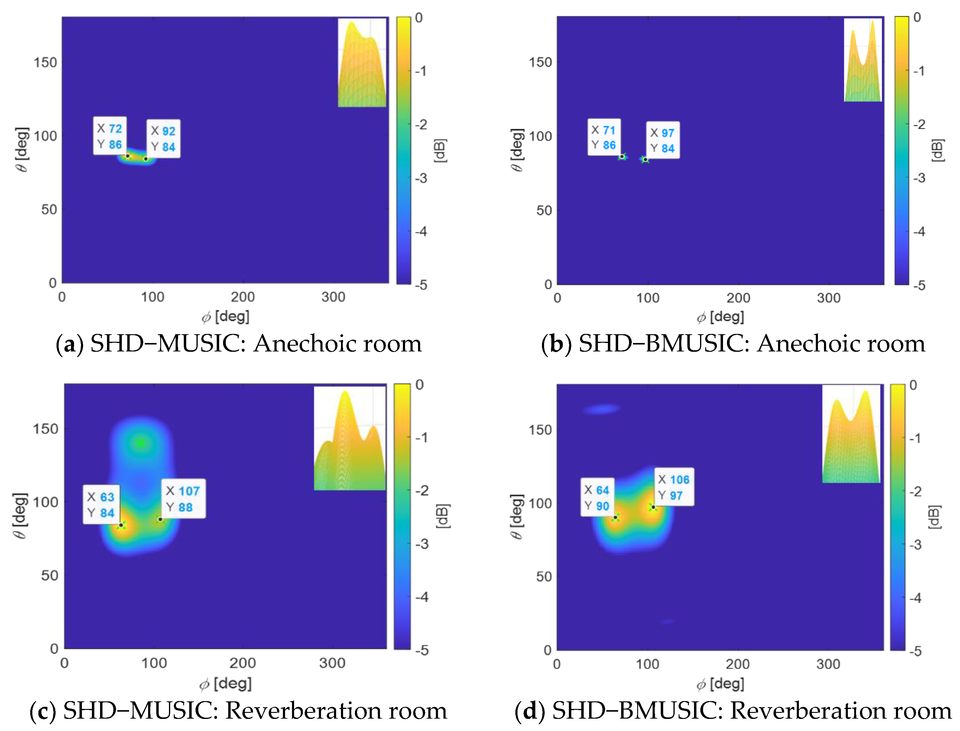
• We verify the superior performance of the proposed algorithm using simulated data as well as field-testing data in real-world situations (anechoic room and reverberant room).

The paper is structured as follows: Section 2 describes the space domain and spherical harmonic domain system models. Section 3 introduces the proposed DOA estimation method. Our experiment findings and discussions are clearly shown in Section 4. Finally, we complete the summary part and conclusions in Section 5.

2. System Models

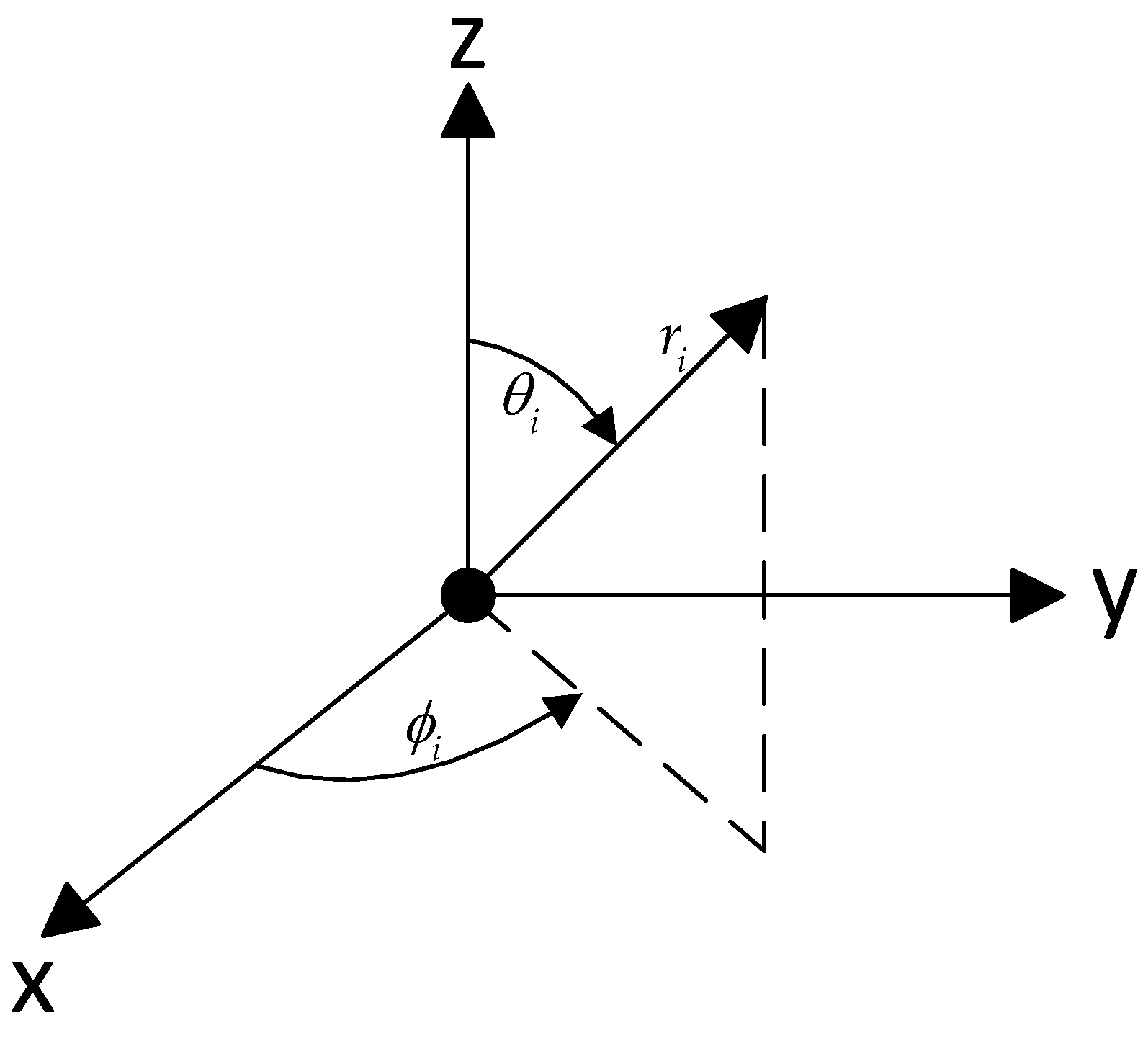
2.1. Space-Domain System Model

We consider a set of spherical microphone arrays consisting of $I$ omnidirectional microphones; $r_i={(r_i\cos {\varphi }_i\sin {\theta }_i,r_i\sin {\varphi }_i\sin {\theta }_i,r_i\cos {\theta }_i)}^T$ denotes the position of the $i$-th microphone of the array. The azimuth $\varphi$ is measured counterclockwise from the x-axis, the elevation angle $\theta$ is measured downward from the z-axis, and $r_i$ represents the distance of the $i$-th microphone to the center of the array. The adopted spherical coordinate system is shown in Figure 1.

There are $L$ far-field sound sources generating plane waves that propagate through space and are picked up by microphones. ${\mathsf{\Psi }}_l=({\theta }_l,{\varphi }_l)$ denotes the direction of propagation of the $l$-th sound source, $k_l=-{(k\cos {\varphi }_l\sin {\theta }_l,k\sin {\varphi }_l\sin {\theta }_l,k\cos {\theta }_l)}^T$ denotes the wave number vector of the $l$-th plane wave. The signal received by the $i$-th microphone in the frequency domain can be expressed as:

$$p_i(k)={\displaystyle \sum _{l=1}^L{v}_i(k,{\mathsf{\Psi }}_l)}{s}_l(k)+n_i(k)$$

(1)

where $v_i(k,{\mathsf{\Psi }}_l)$ denotes the direction of propagation of the $i$-th microphone associated with the $l$-th plane wave; $s_l(k)$ is the amplitude vector of the $l$-th plane wave; $n_i(k)$ is the noise received by the $i$-th microphone. The frequency domain received sound pressure model is expressed in matrix form as follows:

$$p(k)=V(k,\mathsf{\Psi })s(k)+n(k)$$

(2)

where $V(k,\mathsf{\Psi })$ is the $I\times L$ dimensional direction matrix; $s(k)={[s_1(k),\mathrm{\dots },s_L(k)]}^T$ is the $L$ dimensional source signal vector; $n(k)={[n_1(k),\mathrm{\dots },n_I(k)]}^T$ is the $I$ dimensional zero-mean Gaussian white noise vector; and $n(k)$ is assumed to be uncorrelated with $s(k)$. For an open-sphere array (microphones in a free field), $v(k,{\mathsf{\Psi }}_l)$ is denoted as:

$$v(k,{\mathsf{\Psi }}_l)={[e^{-j{k}_l{}^T{r}_1},e^{-j{k}_l{}^T{r}_2},\mathrm{\dots },e^{-j{k}_l{}^T{r}_I}]}^T$$

(3)

2.2. Spherical Harmonic Domain System Model

For the case of rigid spherical array with acoustic scattering [23], the time delay method cannot be used to obtain the sound pressure directly. The sound field modal synthesis method will be introduced to calculate the sound pressure response of the spherical array [24]. According to the Fourier acoustic principle, for a spherical array of order $N$, the sampled sound pressure of the microphone at position $(r,\mathsf{\Omega }),\mathsf{\Omega }=(\theta ,\varphi )$ on the sphere and its spherical harmonic domain (SHD) are expressed as:

$$\begin{array}{l}{p}_{nm}(k,r)={\displaystyle \sum _{i=1}^I{a}_{i}p(k,r,{\mathsf{\Omega }}_i)}{[Y_n^m({\mathsf{\Omega }}_i)]}^{*}\\ p(k,r,\mathsf{\Omega })={\displaystyle \sum _{n=0}^N{\displaystyle \sum _{m=-n}^n{p}_{nm}(k,r)}}{Y}_n^m(\mathsf{\Omega })\end{array}$$

(4)

The spherical Fourier basis function $Y_n^m(\mathsf{\Omega })$ is called the $n$-th order spherical harmonic function (SHF) of the degree of freedom, $m$:

$$Y_n^m(\mathsf{\Omega })=\sqrt{\frac{2n+1}{4\pi }\frac{(n-m)!}{(n+m)!}}{P}_n^m(\cos \theta )e^{im\varphi }$$

(5)

where $P_n^m$ denotes the concatenated Lejeune function; $P_n^m(\cos \theta )$ reflects the effect of $\theta$ on the operation state of the SHF; and $e^{im\varphi }$ reflects the effect of $\varphi$ on the operation state of the SHF. When sampling spherical sound pressure, a spherical sample $({\theta }_i,{\varphi }_i)$ and a sampling weight $a_i$ are given.

To extract the sound field spherical harmonics, the microphone positions are required to satisfy the weighted orthogonality condition. The three types of aliasing-free sampling for spherical array signal processing [25] are equal-angle sampling, Gaussian sampling, and near-uniform sampling. In order to reduce the amount of multi-channel data operation, we use the uniform sampling method which can achieve the minimum number of sampling points. It has a sampling point count of ${(N+1)}^2$ and the sampling weight $a_i=\frac{4\pi }{I}$ is set as a constant.

In the SHD, the frequency and the angular components of the source direction matrix can be separated from each other as follows [20]:

$$v(k,{\mathsf{\Psi }}_l)=y^T({\mathsf{\Omega }}_i)B(kr)y^{*}({\mathsf{\Psi }}_l)$$

(6)

where $y({\mathsf{\Psi }}_l)={[Y_0^0({\mathsf{\Psi }}_l)Y_1^{-1}({\mathsf{\Psi }}_l)Y_1^0({\mathsf{\Psi }}_l)Y_1^1({\mathsf{\Psi }}_l)\mathrm{\dots }{Y}_N^N({\mathsf{\Psi }}_l)]}^T$ is a ${(N+1)}^2$ dimensional vector of SHFs in the sound-source direction, consisting of SHFs of different orders; $y({\mathsf{\Omega }}_i)$ is a ${(N+1)}^2$ dimensional vector of SHFs in the microphone direction, having the same form as $y({\mathsf{\Psi }}_l)$; $B(kr)$ is the modal intensity matrix, which turns out to be a ${(N+1)}^2\times {(N+1)}^2$ dimensional symmetric matrix composed of the spherical modal amplitude response $b_n(kr)$. $b_n(kr)$ is constructed based on the structure of the array as for the open and rigid spherical arrays, respectively:

$$\begin{array}{l}{b}_{n,open}(kr)=4\pi i^n{j}_n(kr)\\ b_{n,rigid}(kr)=4\pi i^n\left(j_n(kr)-\frac{j_n^{\prime }(kr)}{h_n^{\prime }(kr)}{h}_n(kr)\right)\end{array}$$

(7)

where $j_n$ and $h_n$ are the first class $n$ order spherical Bessel function and the second class $n$ order spherical Hankel function, respectively. For the rigid spherical array, the first term of $b_n(kr)$ describes the incident sound field, which is the same as the open spherical array, and the second term of $b_n(kr)$ describes the scattered sound field.

For a plane wave with amplitude $s_l(k)$ and wave number vector $(k,\mathsf{\Psi }),\mathsf{\Psi }=({\theta }_l,{\varphi }_l)$, the sound pressure received at the $i$-th microphone can be expressed as:

$$p_l(k,r,{\mathsf{\Omega }}_i)=y^T({\mathsf{\Omega }}_i)B(kr)y^{*}({\mathsf{\Psi }}_l)s_l(k)$$

(8)

3. Methods

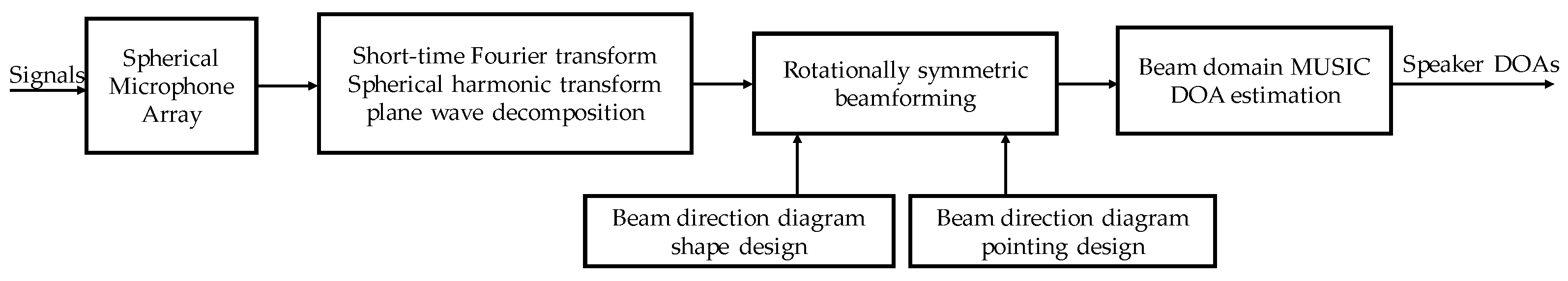
3.1. Framework of the Proposed SHD-BMUSIC

It is known from the literature [19] that the SHD-MUSIC algorithm is sensitive to noise. To address these challenges, we introduce beam design in the SHD and transform the SHD-MUSIC algorithm into the beam space for processing; therefore, we combine the spherical harmonic domain (SHD) with the beam domain (BD). The beamforming is processed in the SHD and the MUSIC spatial spectrum is constructed in the BD. The main advantages are as follows:

• The SHD axisymmetric beamformer is designed to separate the beam steering from the beam weights so that the beam steering can be adjusted arbitrarily without adjusting the beam weights;
• The SHD beam weights can be independent of the signal frequency, without the demands on a special constant beam-width design;
• The frequency and angle components of the source can be decoupled in the SHD, and the frequency smoothing can be used to decouple the coherent source without affecting the DOAs of the sources [14].

The framework of the proposed spherical harmonic domain beam-space MUSIC algorithm (SHD-BMUSIC) DOA estimation scheme is shown in Figure 2.

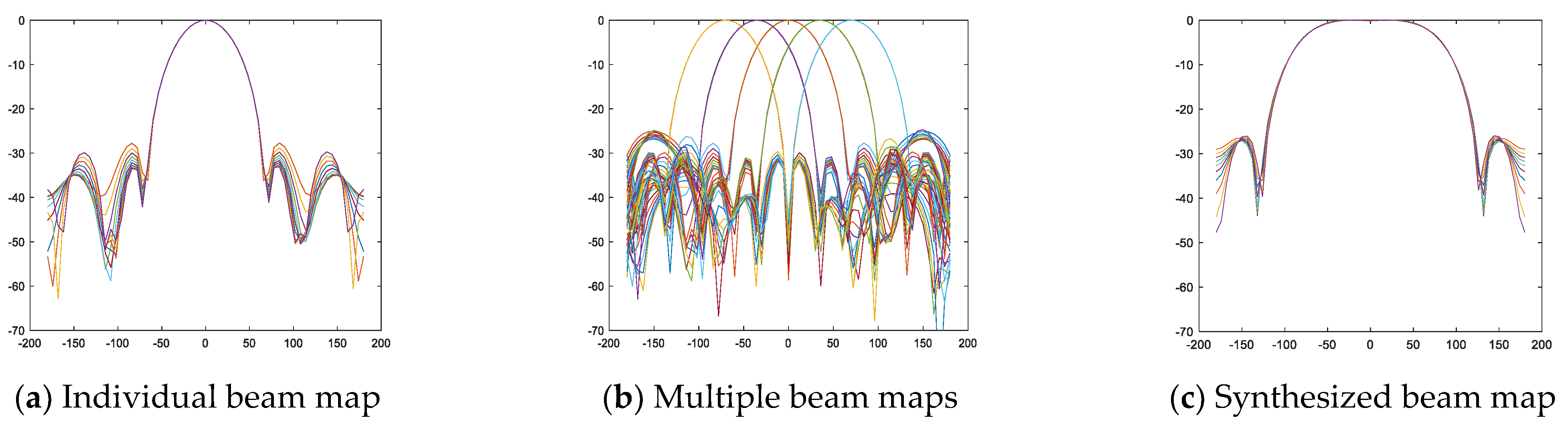
3.2. Beam Weight Design

The beam weight design can be categorized as a single-objective and multi-objective optimization problem. The beam directional map metrics include directionality, white noise gain, side flap level, and main flap width. Although multi-objective formulation descriptions usually do not have closed-form solutions, they can be integrated into numerically solved optimization problems. The multi-objective beam weight design formulation is expressed in the form of a quadratic constraint quadratic planning (QCQP) optimization problem, which is a special case of second-order cone programming (SOCP):

$$\begin{array}{ll}\mathrm{minimize}& w_{nm}^{H}B{w}_{nm}\\ \mathrm{subject}\mathrm{to}& w_{nm}^H{v}_{nm}=1\\ & w_{nm}^{H}A{w}_{nm}\le \frac{1}{WN{G}_{\min }}\\ \mathrm{which}& A=S{S}^H,S=\frac{4\pi }{Q}{Y}^H\\ & B=\frac{1}{4\pi }diag({\left|b_0\right|}^2,{\left|b\right|}_1{}^2,{\left|b_1\right|}^2,{\left|b_1\right|}^2,\mathrm{\dots },{\left|b_N\right|}^2)\end{array}$$

(9)

where $WN{G}_{\min }$ is the lower bound on $WNG$. Matrix $\mathit{S}$ depends on the sampling scheme, for the near-uniform sampling scheme, $S=\frac{4\pi }{Q}{Y}^H$. The matrices $\mathit{A}$ and $\mathit{B}$ are conjugate symmetric matrices. For non-zero vectors $w_{nm}$, $w_{nm}^{H}A{w}_{nm}$, and $w_{nm}^{H}B{w}_{nm}$ is positive definite. $w_{nm}^{H}A{w}_{nm}\le \frac{1}{WN{G}_{\min }}$ denotes the white noise gain constraint. $w_{nm}^H{v}_{nm}=1$ denotes the distortion-free response constraint of the beam direction map in the array view direction. Judging by the satisfaction of distortion-free response constraint and white noise gain constraint, the average response $w_{nm}^{H}B{w}_{nm}$ in all directions of the array is minimized. The beamforming weight $w_{nm}$ is finally derived using a numerical solution method.

3.3. Beam Direction Chart Indicator

The directionality factor ($DF$) is defined as the ratio of the observed directional signal power gain to the all-around uniform arrival signal power gain.

$$DF=\frac{{\left|y({\theta }_k,{\varphi }_k)\right|}^2}{\frac{1}{4\pi }{\displaystyle {\int }_0^{2\pi }{\displaystyle {\int }_0^{\pi }{\left|y(\theta ,\varphi )\right|}^2}}\sin \theta d\theta d\varphi }$$

(10)

where $\mathit{y}({\theta }_k,{\varphi }_k)$ is the response output in the observation direction. $DF$ quantifies the improvement in SNR provided by the array directional response. White noise gain ($WNG$) is defined as the improvement in SNR at the array output compared to the array input and is used as a measure of array robustness:

$$WNG=\frac{{\left|w_{nm}^H{v}_{nm}\right|}^2}{w_{nm}^{H}S{S}^H{w}_{nm}^H}$$

(11)

where $w_{nm}$ is the beamforming weight. Uniform sampling satisfies $S{S}^H=\frac{4\pi }{Q}I$, where $I$ is the unit matrix and $Q$ is the number of sampling samples. $v_{nm}=b_n(kr){[Y_n^m({\theta }_k,{\varphi }_k)]}^{*}$ denotes the array input generated by the plane wave sound field, and can be applied to other arrays such as rigid- or open-sphere arrays by simply modifying $b_n(kr)$. Therefore, the SHD-beamforming system has remarkable flexibility [26].

According to Equation (9), set the white noise gain constraint to $\frac{1}{WN{G}_{\min }}=0.2$ and 2.7 kHz frequency point. The beam weight value $w_{nm}$ is derived based on the QCQP algorithm, since $w_{nm}$ is independent of the signal frequency. Referring to $w_{nm}$, $WNG=22.95dB$ and $DF=24.0dB$ should be set for the entire operating frequency band.

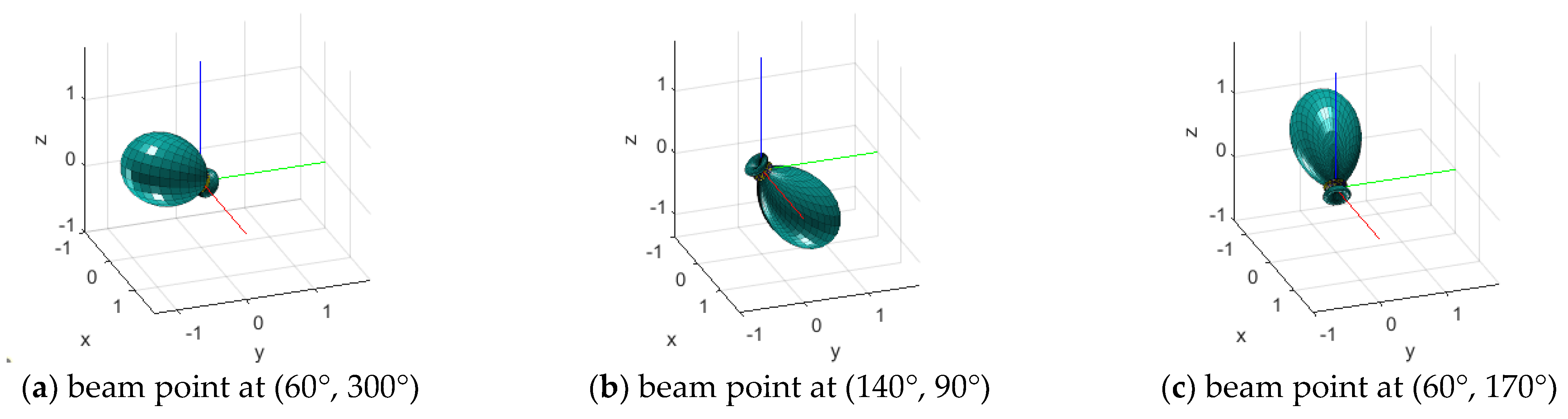
3.4. Rotational Symmetric Beamformer

The SHD-beamforming consists of two parts: spherical harmonic decomposition and SHD weighting summation. If the beam steering angle is to be adjusted, the weighting vector needs to be redesigned. In the beamforming block diagram proposed by Meyer and Elko [27], reducing the beam formation weights to a one-dimensional function. The resulting beam direction map is axisymmetric when viewed from the viewpoint of the axis forming the symmetry. This separates the beam steering adjustment from the weighted value design:

$${\mathit{w}}_{nm,sym}^{*}=\frac{w_{nm}}{b_n(kr)}{Y}_n^m({\theta }_0,{\varphi }_{.0})$$

(12)

The rotationally symmetric beamformer contains two parts: beam guidance and beam synthesis. The weighted value $w_{nm}$ adjusts the beam map shape and the spherical harmonics $Y_n^m({\theta }_0,{\varphi }_{.0})$ adjust the beam steering angle. The rotationally symmetric beamformer with beam weight $w_{nm}$ of Section 3.3 and different beam points $Y_n^m({\theta }_0,{\varphi }_{.0})$ is shown in Figure 3.

A plane wave decomposition (PWD) of ${\mathit{p}}_{nm}(k,r)$, i.e., dividing by the modal intensity $\mathit{B}(kr)$, yields the plane wave amplitude density can be expressed as:

$$a_{nm}(k)=Y^H(\mathsf{\Psi })s(k)+{\overline{n}}_{nm}(k)$$

(13)

The beam response output is obtained using the inner product of axisymmetric beamforming weights ${\mathit{w}}_{nm,sym}^{*}$ with SHD array data ${\mathit{p}}_{nm}(k,r)$:

$$y(kr,\mathsf{\Delta }\mathsf{\Psi })={\displaystyle \sum _{n=0}^N{\displaystyle \sum _{m=-n}^n{p}_{nm}(k,r){\mathit{w}}_{nm,sym}^{*}=}}{\displaystyle \sum _{n=0}^N{\displaystyle \sum _{m=-n}^n{\mathit{w}}_{nm}{a}_{nm}(k)Y_n^m({\theta }_0,{\varphi }_{.0})}}$$

(14)

The beam response $\mathit{y}(kr,\mathsf{\Delta }\mathsf{\Psi })$ is affected by the angle $\mathsf{\Delta }\mathsf{\Psi }$ between the plane wave arrival direction $({\theta }_k,{\varphi }_k)$ and the array view direction $({\theta }_0,{\varphi }_0)$.

3.5. Beam Domain MUSIC

The beam domain MUSIC algorithm forms multiple beams in the spatial sector of interest with the number of beams between the number of sources and the number of microphones [28]. Different pointing beams are used for synthesis to cover the target area, which forms a $D\times {(N+1)}^2$ dimensional axisymmetric beamforming matrix $W_{nm,sym}=[{\mathit{w}}_{nm1,sym},\mathrm{\dots },{\mathit{w}}_{nmD,sym}]$. The 2D preformed multi-beam matrix is shown in Figure 4.

If the beamforming matrix $W_{nm,sym}$ does not satisfy $W_{nm,sym}^H{W}_{nm,sym}=I$, the standard orthogonalization needs to be performed on it as follows:

$${\overline{W}}_{nm,sym}=W_{nm,sym}{(W_{nm,sym}^H{W}_{nm,sym})}^{-1/2}$$

(15)

The beam response vector, obtained using the inner product of the beamforming weighting matrix and SHD array data, is expressed in matrix form:

$$y(kr,\mathsf{\Delta }\mathsf{\Psi })={\overline{W}}_{nm,sym}^H{p}_{nm}(k,r)$$

(16)

The beam domain data covariance matrix, $S_y(k)=E\{y(kr,\mathsf{\Delta }\mathsf{\Psi })y^H(kr,\mathsf{\Delta }\mathsf{\Psi })\}$, is reduced to $D\times D$ dimensions and the operations of the feature decomposition are reduced to $o(D^3)$. Therefore, the dimension-reduction beam-space processing eases the operations of the subspace algorithm.

Frequency smoothing (FS) can be applied as a straightforward average by assuming frequency independence of the (mode strength compensated) array manifold [29]. We de-correlate the coherent source signal by implementing FS that computes the smoothed covariance matrix as the average of covariance matrices at different frequency sectors. Then, the smoothed beam response covariance matrix ${\tilde{S}}_y=\frac{1}{K}{\displaystyle \sum _{q=1}^K{S}_y(k_q)}$ is obtained.

The eigenvalue decomposition of ${\tilde{S}}_y$ is performed to obtain the noise subspace and the signal subspace in the beam domain. The BD-MUSIC spatial pseudo-spectral function is constructed using the orthogonality of the beam scan vector $b(\mathsf{\Psi })={\overline{W}}_{nm,sym}^{H}y(\mathsf{\Psi })$ and beam domain noise subspace $E_{nm}$. The equations can be summarized as follows:

$$P_{SHD-BMUSIC}(\mathsf{\Psi })=\frac{b^H(\mathsf{\Psi })b(\mathsf{\Psi })}{b^H(\mathsf{\Psi }){\overline{W}}_{nm,sym}^H{E}_{nm}{({\overline{W}}_{nm,sym}^H{E}_{nm})}^{H}b(\mathsf{\Psi })}$$

(17)

Finally, the spectral peak search is carried out and the direction corresponding to the peak is the DOA of the sound sources.

4. Experiment

4.1. Simulation Parameter Settings

We simulated the room impulse response (RIRs) between an omnidirectional source and a microphone in a reverberant environment using the image-source method modified to account for the scattering of a rigid sphere [23]. Multiple randomly selected audios from the TIMIT database were used as a simulated source of the original vocalizations. The original audio signal was a pure voice signal of 4 s duration with a sampling rate of 16 kHz. The indoor 3D empty room size was set to $4 \mathrm{m}\times 6 \mathrm{m}\times 3 \mathrm{m}$. The radius of the sphere array $r$ was 0.042 m, placed in the middle of the room, and the distance of the original sound sources from the center of the sphere array was 1 m. The spherical array was configured as a rigid sphere using uniform sampling weights. The order $N$ of the spherical harmonic function was taken as three.

The signals received of the sphere array were obtained by convolving the original audio with the RIRs and by adding a certain SNR of Gaussian white noise. The signals received were transformed to the time–frequency domain using the short-time Fourier transform (STFT). The frame length of STFT was 16 ms, and the selected window function was a Hamming window with a window length of 256 points and a frame overlap of 50%. Then, we carried out a spherical harmonic transform in the used frequency band. A disadvantage of rigid spherical arrays is the low-frequency performance, so excessive noise amplification at lower frequencies due to modal strength compensation needs to be avoided [29]. According to the spatial aliasing $kr<N$, the upper-frequency limit is around 5 kHz. Thirty frequency bins ranging from 2700 Hz to 3600 Hz were used to perform the spherical harmonic transform to obtain the SHD sound pressure data. Finally, DOA estimation algorithms were executed separately to obtain the DOAs of the sound sources. The azimuthal accuracy and elevation angle accuracy of the spectrum peak search were 1 degree. The localization performances of the SHD-MUSIC and SHD-BMUSIC are compared in these different SNR levels and reverberation time (RT) environments.

4.2. DOA Estimated Evaluation Metrics

To evaluate the algorithm fairly, the performances of the algorithm using two qualitative metrics were measured. Fifty Monte Carlo simulation trials were performed in each sound field condition.

The first metric was the average number of detected sources, which analyzed whether the DOA estimation algorithm was supposed to detect the target source. For each detection, the target source was detected if the deviation between the estimated angle and the true angle was set within 20°. The number of sources detected each time was statistically averaged to obtain the average number of detected sources.

When multiple sources can be correctly distinguished, we used a second evaluation metric of the average root mean square error (RMSE):

$$RMSE=\sqrt{\frac{{\displaystyle \sum _{m=1}^M{\displaystyle \sum _{l=1}^L{\left(\left|{\theta }_{ori}^m(l)-{\theta }_{est}^m(l)\right|+\left|{\varphi }_{ori}^m(l)-{\varphi }_{est}^m(l)\right|\right)}^2}}}{LM}}$$

(18)

where $L$ is the number of sound sources; $M$ is the number of cases that successfully detect all the $L$ sound sources.; $({\theta }_{ori}^m(l),{\varphi }_{ori}^m(l))$ is the true position of the $l$-th source in the $m$-th trial; $({\theta }_{est}^m(l),{\varphi }_{est}^m(l))$ is the estimated position of the $l$-th source in the $m$-th trial. The average of the estimated positions of all trials is taken as the final estimated position $({\overline{\theta }}_{est}^{}(l),{\overline{\varphi }}_{est}^{}(l))$ of the $l$th source. The average RMSE determines the deviation between the true position and the estimated position and is used to analyze the accuracy of the localization algorithm. Only the RMSE of the positioned angle of the detected signal is considered.

4.3. Simulation Testing Results

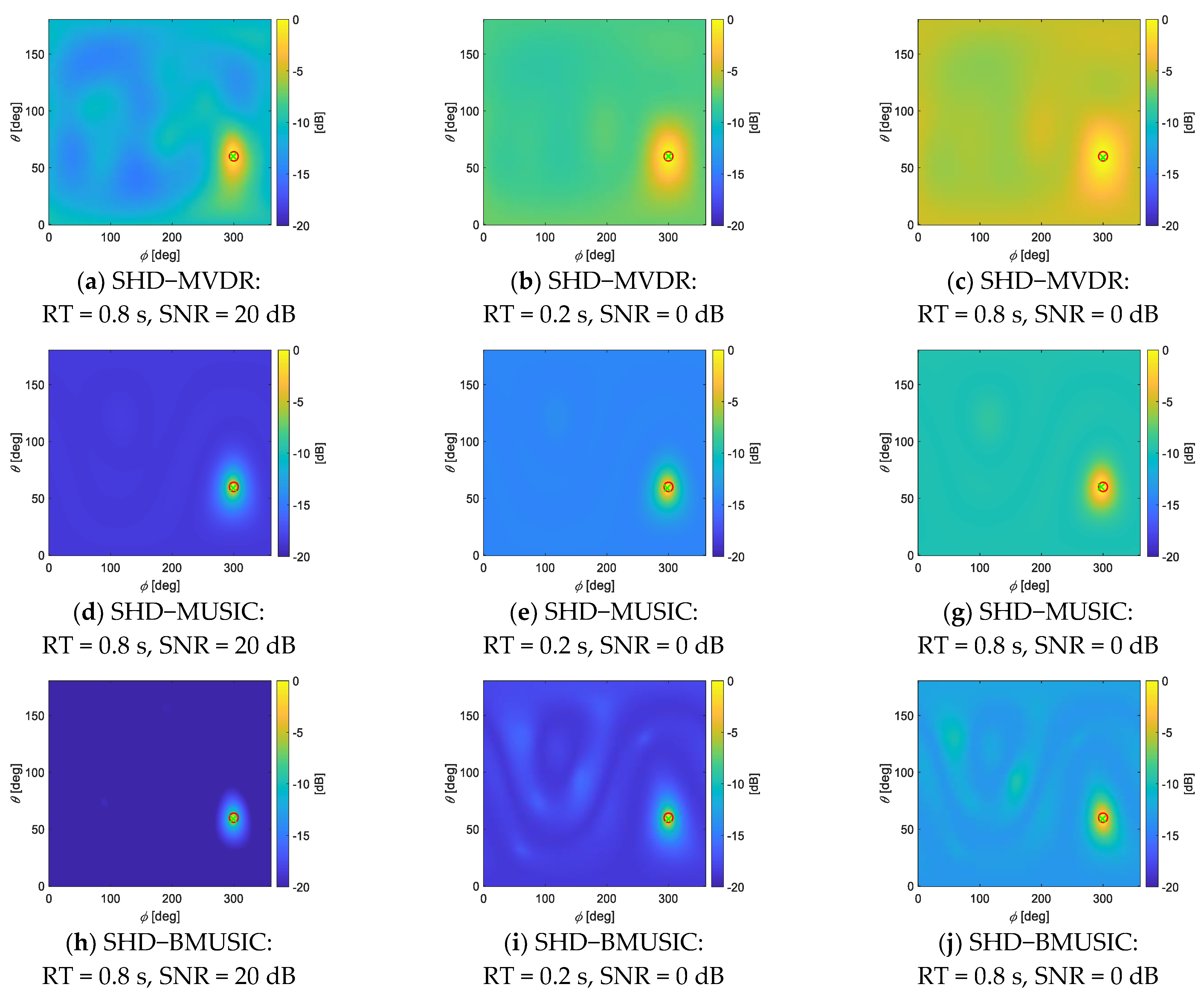
4.3.1. Single-Source Localization Algorithm Verification

First, the estimation results of the algorithms for spherical harmonic domain-minimum variance distortion-free response (SHD-MVDR) [12], SHD-MUSIC, and SHD-BMUSIC are compared for the single-source case. Aiming at minimizing the contribution of noise and any arriving signals from other directions, the MVDR method is supposed to maintain a fixed gain in the look direction. Three groups of single-source experiments with different sound field environments were tested. The sound source was located at (60°, 300°). The sound field conditions were high reverberation (RT = 0.8 s, SNR = 20 dB), low SNR (RT = 0.2 s, SNR = 0 dB), and high-reverberation low-SNR (RT = 0.8 s, SNR = 0 dB). For the SHD-BMUSIC algorithm, five beams were formed to cover the area where the target sound source was located. The estimated spatial spectrum of the single source for the three algorithms is shown in Figure 5.

The spatial spectrum of the single source showed that all three algorithms successfully estimated the location of the single source in different environments. However, the spatial spectral peaks of SHD-BMUSIC were both sharper than SHD-MUSIC and SHD-MVDR and the spatial spectral gain was higher. It was quite convincing that the SHD-BMUSIC algorithm suppressed the noise outside the beam region under these circumstances and the SNR outputs were improved.

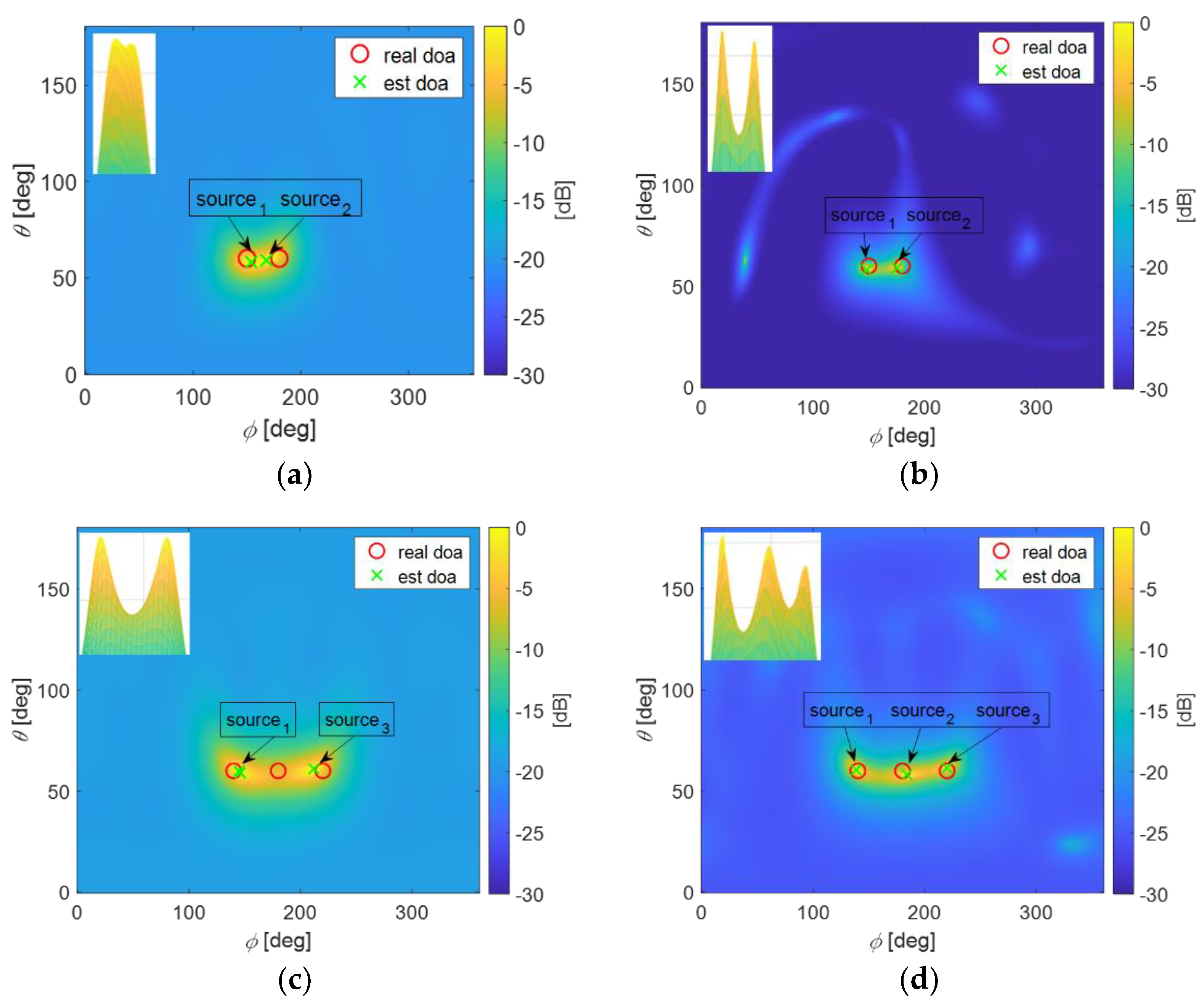
4.3.2. Adjacent Sound Sources Localization Algorithm Verification

In this section, we verify that the SHD-BMUSIC was able to distinguish the locations of multiple adjacent sound sources with higher source identification accuracy compared to SHD-MUSIC. Two sets of experiments with the adjacent sound sources were performed. The first set of experiments set up sound source 1 at (60°, 150°) and sound source 2 at (60°, 180°). The second group of experiments set up sound source 1 at (60°, 140°), sound source 2 at (60°, 180°), and sound source 3 at (60°, 220°). Both experiments were conducted in an environment with RT = 0.3 s and SNR = 20 dB. For the SHD-BMUSIC algorithm, for the first set of experiments, five beams were used to cover the area where two sources were located. For the second set of experiments, seven beams were used to cover the area where the three sources were located. The spatial spectra of the adjacent sound sources for both algorithms are shown in Figure 6.

It is quite convincing that the algorithm proposed has a better discriminative ability than SHD-MUSIC.

Table 1. Localization results and errors for two adjacent sound sources at SNR = 20 dB, RT = 0.3 s.

Methods	$({\overline{\mathit{\theta }}}_{\mathit{e}\mathit{s}\mathit{t}}^{}(1),{\overline{\mathit{\varphi }}}_{\mathit{e}\mathit{s}\mathit{t}}^{}(1))$	$({\overline{\mathit{\theta }}}_{\mathit{e}\mathit{s}\mathit{t}}^{}(2),{\overline{\mathit{\varphi }}}_{\mathit{e}\mathit{s}\mathit{t}}^{}(2))$	Average Number of Detected Sources	Average RMSE
SHD-MUSIC	(58°, 155°)	(59°, 171°)	1.45	5.4261
SHD-BMUSIC	(59°, 149°)	(58°, 173°)	1.96	4.6440

and

Table 2. Localization results and errors for three adjacent sound sources at SNR = 20 dB, RT = 0.3 s.

Methods	$({\overline{\mathit{\theta }}}_{\mathit{e}\mathit{s}\mathit{t}}^{}(1),{\overline{\mathit{\varphi }}}_{\mathit{e}\mathit{s}\mathit{t}}^{}(1))$	$({\overline{\mathit{\theta }}}_{\mathit{e}\mathit{s}\mathit{t}}^{}(2),{\overline{\mathit{\varphi }}}_{\mathit{e}\mathit{s}\mathit{t}}^{}(2))$	$({\overline{\mathit{\theta }}}_{\mathit{e}\mathit{s}\mathit{t}}^{}(3),{\overline{\mathit{\varphi }}}_{\mathit{e}\mathit{s}\mathit{t}}^{}(3))$	Average Number of Detected Sources	Average RMSE
SHD-MUSIC	(60°, 145°)	(59°, 147°)	(61°, 212°)	2.06	3.4549
SHD-BMUSIC	(60°, 139°)	(58°, 185°)	(62°, 221°)	2.84	2.8284

show the experimental statistics for the two cases, respectively.

As shown in Table 1 and Table 2, for the first set of conditions, both algorithms succeeded most of the time in distinguishing two adjacent sound sources. However, SHD-BMUSIC had a higher average number of detected sources and a lower average RMSE. For the second set of conditions, SHD-MUSIC was basically unable to completely estimate the three adjacent sound sources. The intermediate source was not successfully detected in most cases, resulting in a small average number of detected sources for SHD-MUSIC. In contrast, SHD-BMUSIC was able to detect all three sound sources in most tests. In the tests where all sound sources were successfully discriminated, SHD-BMUSIC also had a smaller average RMSE. As a result, SHD-BMUSIC improved the accuracy of sound source location estimation and had a higher adjacent source discrimination capability. The increase in position resolution was the gain from the beamforming operation.

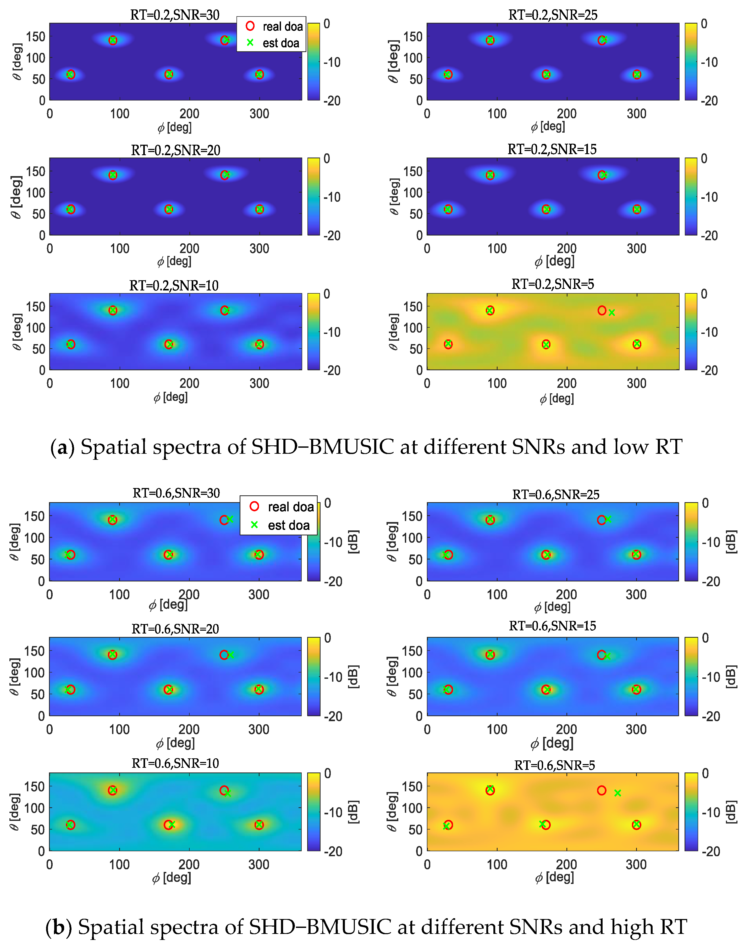
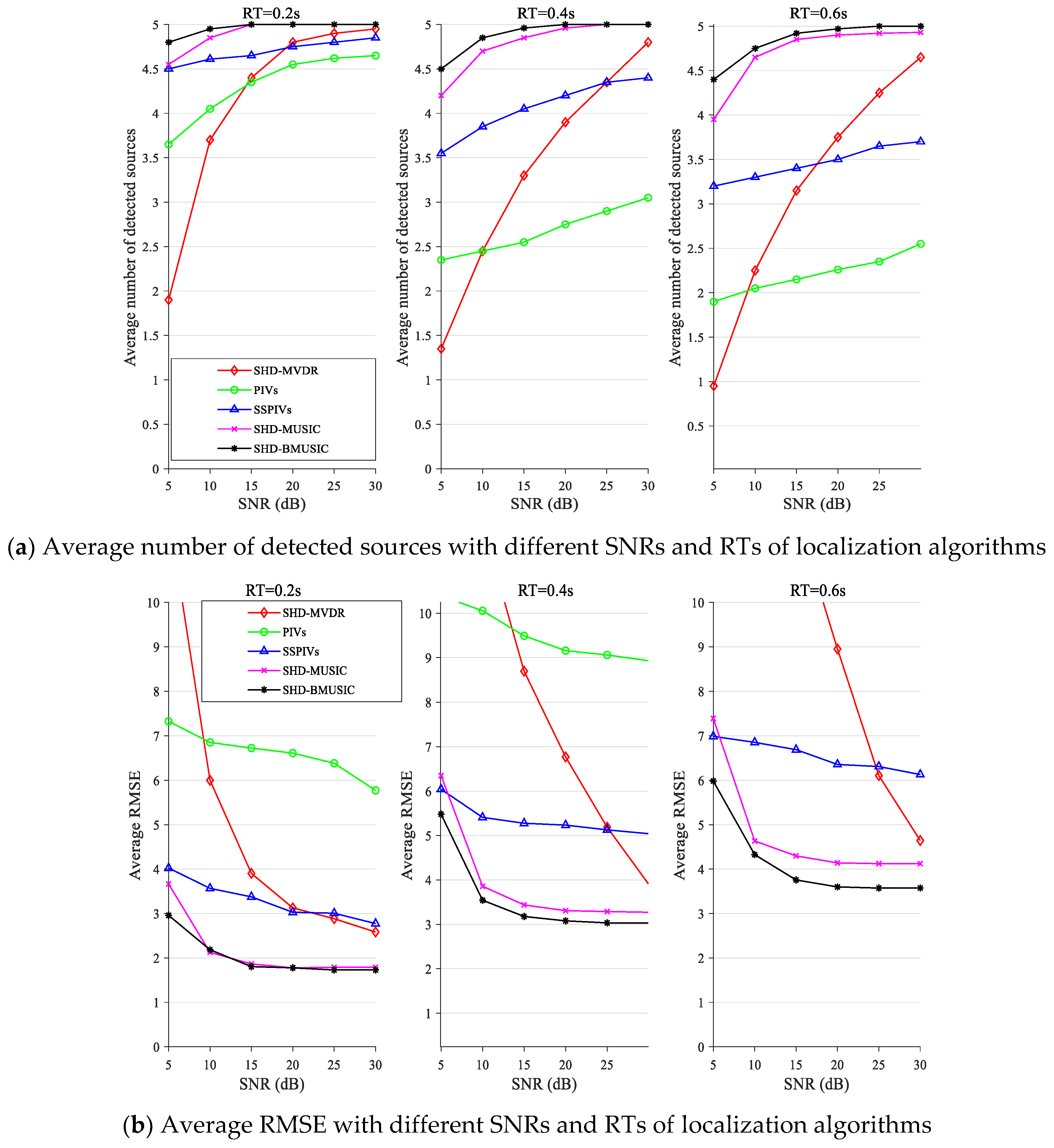
4.3.3. Multi-Source Localization Algorithm Verification at Different SNRs and RTs

To verify the performance of the SHD-BMUSIC algorithm in the reverberation-noise sound field, we considered the positioning results under different reverberation durations and SNR levels. There were five sources emitting simultaneously, and the source locations were (60°, 300°), (140°, 90°), (60°, 170°), (140°, 250°), and (60°, 30°). There were 25 beams used to form five new separate beams to the source area and to cover the target area. The spatial spectra of SHD-BMUSIC at different SNRs and RTs are shown in Figure 7.

The statistical results of SHD-MVDR, PIVs [29], SSPIVs [29], SHD-MUSIC, and SHD-BMUSIC algorithms were compared for multi-source case testing. Figure 8 shows the average results of the tests with five sources for each combination of SNR and RT.

As seen in Figure 8, overall, the performance of the localization algorithm showed a certain degree of decline as the SNR decreased and the RT increased. The performance of SHD-MVDR was seriously affected by reverberation and noise. SSPIVs improved the shortcomings of PIVs which were severely affected by reverberation. PIVs and SSPIVs had shorter running times because they were not expected to carry out a spectral peak search. The SHD-MUSIC and SHD-BMUSIC, which use frequency smoothing, had strong adaptability to reverberation. Due to the gain from beamforming, the proposed algorithm had better sound-source detection capability and localization accuracy than the rest of the algorithms, showing better anti-noise and anti-reverberation performance.

4.4. Field Testing Results

The spherical microphone equipment was used to collect the recording data in a standard anechoic and reverberant room. Each audio segment was recorded for 4 s and the rest of the parameter settings were the same as the simulation parameter settings. The actual spherical microphone array we used and the actual experimental room for field testing are shown in Figure 9.

First of all, the case of the single-sound source was tested. The source in the anechoic room was located at (90°, 190°); the source in the reverberant room was located at (90°, 220°). The spatial spectra estimated by the two algorithms are shown in Figure 10.

Then, the case of the adjacent dual-sound sources was tested. The locations of the two sources in the anechoic and reverberant rooms were (90°, 70°) and (90°, 100°). The estimated spatial spectra of the two algorithms are shown in Figure 11.

Finally, it is promising to conclude that both algorithms are better at estimating the location of a single source in an anechoic room. The SHD-BMUSIC had sharper peaks and lower estimation errors. In the reverberation room, SHD-MUSIC showed additional excess peaks due to reverberant reflected sound in adjacent dual-source experiments. This made it easy for the algorithm to mistake the pseudo-peaks for the direction of the sound source, leading to an incorrect estimation of the sound source location. However, SHD-BMUSIC did not have the phenomenon of redundant pseudo-peaks. This was because the beamforming suppressed the excess reflected sound outside the source region, thus improving the reverberation resistance of the algorithm.

5. Conclusions

In this paper, we use a spherical harmonic domain beam-space MUSIC algorithm to solve the multi-source DOA estimation problem in harsh environments where reverberation and noise coexist. The designed spherical harmonic-domain beam is not only easy to implement, with flexible adjustment of steering, but also reduces the matrix dimension to reduce the amount of eigen-decomposition operations. From the experimental results, it can be seen that the SHD-BMUSIC algorithm has some advantages over the SHD-MUSIC algorithm without the beam domain strategy. Its offline construction of the beam does not increase the time consumption of online real-time positioning. Instead, it enables online localization with sharper spatial spectral peaks, more robust multi-source localization capability, and adjacent source discrimination. We will further optimize the design in the direction of beamforming and the MUSIC algorithm to better solve the problem of locating and tracking multiple adjacent sound sources in high-reverberation and high-noise environments.

References

1. Evers, C.; Lollmann, H.W.; Mellmann, H.; Schmidt, A.; Barfuss, H.; Naylor, P.A.; Kellermann, W. The LOCATA Challenge: Acoustic Source Localization and Tracking. IEEE/ACM Trans. Audio Speech Lang. Process. 2020, 28, 1620–1643. [Google Scholar] [CrossRef]
2. He, H.; Wu, L.; Lu, J.; Qiu, X.; Chen, J. Time Difference of Arrival Estimation Exploiting Multichannel Spatio-Temporal Prediction. IEEE Trans. Audio Speech Lang. Process. 2013, 21, 463–475. [Google Scholar] [CrossRef]
3. Diaz-Guerra, D.; Miguel, A.; Beltran, J.R. Robust Sound Source Tracking Using SRP-PHAT and 3D Convolutional Neural Networks. IEEE/ACM Trans. Audio Speech Lang. Process. 2021, 29, 300–311. [Google Scholar] [CrossRef]
4. Jaafer, Z.; Goli, S.; Elameer, A.S. Performance Analysis of Beam Scan, MIN-NORM, Music and Mvdr DOA Estimation Algorithms. In Proceedings of the 2018 International Conference on Engineering Technology and their Applications (IICETA), Al-Najaf, Iraq, 8–9 May 2018; pp. 72–76. [Google Scholar]
5. Xu, C.; Xiao, X.; Sun, S.; Rao, W.; Chng, E.S.; Li, H. Weighted Spatial Covariance Matrix Estimation for MUSIC Based TDOA Estimation of Speech Source. In Proceedings of the Interspeech 2017, ISCA, Stockholm, Sweden, 20–24 August 2017; pp. 1894–1898. [Google Scholar]
6. Tervo, S.; Politis, A. Direction of Arrival Estimation of Reflections from Room Impulse Responses Using a Spherical Microphone Array. IEEE/ACM Trans. Audio Speech Lang. Process. 2015, 23, 1539–1551. [Google Scholar] [CrossRef]
7. Hu, Y.; Lu, J.; Qiu, X. Direction of Arrival Estimation of Multiple Acoustic Sources Using a Maximum Likelihood Method in the Spherical Harmonic Domain. Appl. Acoust. 2018, 135, 85–90. [Google Scholar] [CrossRef]
8. Choi, J.-W.; Zotter, F.; Jo, B.; Yoo, J.-H. Multiarray Eigenbeam-ESPRIT for 3D Sound Source Localization With Multiple Spherical Microphone Arrays. IEEE/ACM Trans. Audio Speech Lang. Process. 2022, 30, 2310–2325. [Google Scholar] [CrossRef]
9. Yadav, S.K.; George, N.V. Sparse Distortionless Modal Beamforming for Spherical Microphone Arrays. IEEE Signal Process. Lett. 2022, 29, 2068–2072. [Google Scholar] [CrossRef]
10. Yan, S.; Sun, H.; Svensson, U.P.; Ma, X.; Hovem, J.M. Optimal Modal Beamforming for Spherical Microphone Arrays. IEEE Trans. Audio Speech Lang. Process. 2011, 19, 361–371. [Google Scholar] [CrossRef]
11. Kumar, L.; Hegde, R.M. Near-Field Acoustic Source Localization and Beamforming in Spherical Harmonics Domain. IEEE Trans. Signal Process. 2016, 64, 3351–3361. [Google Scholar] [CrossRef]
12. Khaykin, D.; Rafaely, B. Acoustic Analysis by Spherical Microphone Array Processing of Room Impulse Responses. J. Acoust. Soc. Am. 2012, 132, 261–270. [Google Scholar] [CrossRef]
13. Kumar, L.; Bi, G.; Hegde, R.M. The Spherical Harmonics Root-Music. In Proceedings of the 2016 IEEE International Conference on Acoustics, Speech and Signal Processing (ICASSP), Shanghai, China, 20–25 March 2016; pp. 3046–3050. [Google Scholar]
14. Khaykin, D.; Rafaely, B. Coherent Signals Direction-of-Arrival Estimation Using a Spherical Microphone Array: Frequency Smoothing Approach. In Proceedings of the 2009 IEEE Workshop on Applications of Signal Processing to Audio and Acoustics, New Paltz, NY, USA, 17–20 October 2009; pp. 221–224. [Google Scholar]
15. Pan, X.; Wang, H.; Lou, Z.; Su, Y. Fast Direction-of-Arrival Estimation Algorithm for Multiple Wideband Acoustic Sources Using Multiple Open Spherical Arrays. Appl. Acoust. 2018, 136, 41–47. [Google Scholar] [CrossRef]
16. Samarasinghe, P.; Abhayapala, T.; Poletti, M. Wavefield Analysis Over Large Areas Using Distributed Higher Order Microphones. IEEE/ACM Trans. Audio Speech Lang. Process. 2014, 22, 647–658. [Google Scholar] [CrossRef]
17. Coteli, M.B.; Hacihabiboglu, H. Multiple Sound Source Localization with Rigid Spherical Microphone Arrays via Residual Energy Test. In Proceedings of the ICASSP 2019—2019 IEEE International Conference on Acoustics, Speech and Signal Processing (ICASSP), Brighton, UK, 12–17 May 2019; pp. 790–794. [Google Scholar]
18. Jin, C.T.; Epain, N.; Parthy, A. Design, Optimization and Evaluation of a Dual-Radius Spherical Microphone Array. IEEE/ACM Trans. Audio Speech Lang. Process. 2014, 22, 193–204. [Google Scholar] [CrossRef]
19. Hu, Y.; Abhayapala, T.D.; Samarasinghe, P.N. Multiple Source Direction of Arrival Estimations Using Relative Sound Pressure Based MUSIC. IEEE/ACM Trans. Audio Speech Lang. Process. 2021, 29, 253–264. [Google Scholar] [CrossRef]
20. Nadiri, O.; Rafaely, B. Localization of Multiple Speakers under High Reverberation Using a Spherical Microphone Array and the Direct-Path Dominance Test. IEEE/ACM Trans. Audio Speech Lang. Process. 2014, 22, 1494–1505. [Google Scholar] [CrossRef]
21. Madmoni, L.; Rafaely, B. Direction of Arrival Estimation for Reverberant Speech Based on Enhanced Decomposition of the Direct Sound. IEEE J. Sel. Top. Signal Process. 2019, 13, 131–142. [Google Scholar] [CrossRef]
22. Rafaely, B.; Alhaiany, K. Speaker Localization Using Direct Path Dominance Test Based on Sound Field Directivity. Signal Processing 2018, 143, 42–47. [Google Scholar] [CrossRef]
23. Jarrett, D.P.; Habets, E.A.P.; Thomas, M.R.P.; Naylor, P.A. Rigid Sphere Room Impulse Response Simulation: Algorithm and Applications. J. Acoust. Soc. Am. 2012, 132, 1462–1472. [Google Scholar] [CrossRef] [Green Version]
24. Hu, Y.; Samarasinghe, P.N.; Abhayapala, T.D.; Dickins, G. Modeling Characteristics of Real Loudsouers Using Various Acoustic Models: Modal-Domain Approaches. In Proceedings of the ICASSP 2019—2019 IEEE International Conference on Acoustics, Speech and Signal Processing (ICASSP), Brighton, UK, 12–17 May 2019; pp. 561–565. [Google Scholar]
25. Rafaely, B.; Weiss, B.; Bachmat, E. Spatial Aliasing in Spherical Microphone Arrays. IEEE Trans. Signal Process. 2007, 55, 1003–1010. [Google Scholar] [CrossRef]
26. Wang, L.; Zhu, J. Flexible Beampattern Design Algorithm for Spherical Microphone Arrays. IEEE Access 2019, 7, 139488–139498. [Google Scholar] [CrossRef]
27. Meyer, J.; Elko, G. A Highly Scalable Spherical Microphone Array Based on an Orthonormal Decomposition of the Soundfield. In Proceedings of the IEEE International Conference on Acoustics Speech and Signal Processing, Orlando, FL, USA, 13–17 May 2002; pp. II-1781–II-1784. [Google Scholar]
28. Li, X.; Yan, S.; Ma, X.; Hou, C. Spherical Harmonics MUSIC versus Conventional MUSIC. Appl. Acoust. 2011, 72, 646–652. [Google Scholar] [CrossRef]
29. Moore, A.H.; Evers, C.; Naylor, P.A. Direction of Arrival Estimation in the Spherical Harmonic Domain Using Subspace Pseudointensity Vectors. IEEE/ACM Trans. Audio Speech Lang. Process. 2017, 25, 178–192. [Google Scholar] [CrossRef]
Figure 1. Defined spherical coordinate system.
Symmetry 15 00187 g001
Figure 2. Flow chart of DOAs estimation scheme for indoor sound sources.
Symmetry 15 00187 g002
Figure 3. Axisymmetric beam diagram with the same beam shape and different beam steering.
Symmetry 15 00187 g003
Figure 4. Two-dimensional form of the preformed multi-beam directional map.
Symmetry 15 00187 g004
Figure 5. Spatial spectra of single sound source in different acoustic environments.
Symmetry 15 00187 g005
Figure 6. Spatial spectra of adjacent sound sources at SNR = 20 dB, RT = 0.3 s. (a) SHD−MUSIC: two adjacent sound sources; (b) SHD−BMUSIC: two adjacent sound sources; (c) SHD−MUSIC: three adjacent sound sources; (d) SHD−BMUSIC: three adjacent sound sources.
Symmetry 15 00187 g006
Figure 7. Multi-source spatial spectra of SHD−BMUSIC at different SNRs and RTs (five sources).
Symmetry 15 00187 g007
Figure 8. Line graph of the statistical trials of the localization algorithm (five sources).
Symmetry 15 00187 g008
Figure 9. Experimental equipment and different field-testing scenarios.
Symmetry 15 00187 g009
Figure 10. Spatial spectra for actual testing of single-sound source.
Symmetry 15 00187 g010
Figure 11. Spatial spectra for actual testing of adjacent dual-sound sources.
Symmetry 15 00187 g011