Noether Symmetries and Conservation Laws in Static Cylindrically Symmetric Spacetimes via Rif Tree Approach

Abstract

A new approach is adopted to completely classify the Lagrangian associated with the static cylindrically symmetric spacetime metric via Noether symmetries. The determining equations representing Noether symmetries are analyzed using a Maple algorithm that imposes different conditions on metric coefficients under which static cylindrically symmetric spacetimes admit Noether symmetries of different dimensions. These conditions are used to solve the determining equations, giving the explicit form of vector fields representing Noether symmetries. The obtained Noether symmetry generators are used in Noether’s theorem to find the expressions for corresponding conservation laws. The singularity of the obtained metrics is discussed by finding their Kretschmann scalar.

1. Introduction

In 1915, Albert Einstein proposed a gravitational theory, known as the theory of general relativity. In contrast to Newton’s theory, in which gravity was considered as a force of attraction between massive objects, the general theory of relativity states that the observed gravitational effect between masses occurs because of their warping of spacetime. A precise relationship between the properties of matter and spacetime geometry is provided by Einstein’s field equations (EFEs), which are ten partial differential equations and are considered as the centerpiece of general relativity. The concepts of Riemannian geometry are used to formulate these equations such that the spacetime metric describes the geometric properties of spacetime.

The solutions of EFEs are those spacetime metrics that result from solving these equations and correspond to some physically realistic source of energy-momentum tensor. Finding the exact solutions of these equations is not an easy task, the reason being their non-linear nature. In literature, the exact solutions of these equations are found using some assumptions [1], the most common being the imposition of symmetry restrictions on the metric of spacetime. A specific type of vector fields, known as Killing vector fields (KVFs), is used to represent these symmetry restrictions. These vector fields preserve the metric of spacetime and satisfy the relation [2]:

$$g_{\alpha \beta ,\gamma }{V}^{\gamma }+g_{\alpha \gamma }{V}_{,\beta }^{\gamma }+g_{\beta \gamma }{V}_{,\alpha }^{\gamma }=0.$$

(1)

In the above equation, V is a KVF, $g_{\alpha \beta }$ is the metric tensor and $\alpha$ and $\beta$ varies from 0 to 3. Killing vector fields are directly related with conservation laws. For example, every timelike KVF gives the conservation of energy, spacelike KVFs correspond to linear momentum, while a rotational KVF yields angular momentum in a spacetime.

Though KVFs are crucial in studying the conservation laws in spacetimes, sometimes they do not provide a complete list of conservation laws. In such a case, one needs some conformal transformation that is applied to the metric of spacetime and then KVFs are calculated for the conformally transformed metric. For example, the Friedmann metric does not possess a timelike KVF giving conservation of energy; however, an appropriate conformal transformation can be applied to this metric and then KVFs of the tranformed metric can be found to recover the energy conservation. This process is equivalent to find the conformal vector fields (CVFs) of the original metric directly. A conformal vector field V is defined by [2]:

$$g_{\alpha \beta ,\gamma }{V}^{\gamma }+g_{\alpha \gamma }{V}_{,\beta }^{\gamma }+g_{\beta \gamma }{V}_{,\alpha }^{\gamma }=2\lambda \left(x^a\right),$$

(2)

where $\lambda$ denotes a smooth map that depends on spacetime coordinates. In particular, if $\lambda$ is a constant function, the conformal vector field V becomes a homothetic vector field (HVF). For different geometries represented by spacetime metrics, the above defined symmetries are widely studied in the literature [3,4,5,6,7,8,9,10,11].

In addition to the above defined spacetime symmetries, there is another symmetry, known as Noether symmetry, that is found to be very helpful in the classification of Lagrangians associated with spacetime metrics as well as in the study of differential equations. As their role in finding the solution of complicated differential equations is concerned, Noether symmetries help in reducing their orders, the number of independent variables and in linearization of nonlinear differential equations. Moreover, the well-known Noether’s theorem provides a direct relation between Noether symmetries and conservation laws.

If V is a vector field of the form $V=\xi {\partial }_s+V^a{\partial }_{x^a}$ and $V^{\left[1\right]}=V+V_{,s}^a{\partial }_{\dot{x^a}}$ with $V_{,s}^a=D{V}^a-\dot{x^a}D\xi$ is its first prolongation, then V is called a Noether symmetry of the Lagrangian $L(s,x^a,\dot{x^a})$ if we can find a function $F(s,x^a),$ called gauge function, such that:

$$V^{\left[1\right]}L+\left(D_s\xi \right)L=D_{s}F,$$

(3)

where $D_s={\partial }_s+\dot{x^a}{\partial }_{x^a},$$\xi$ and $V^a$ depend on the geodesics parameter s and the four spacetime coordinates $x^a$ and the derivative w.r.t s is denoted by a dot. For a spacetime metric $d{s}^2=g_{\alpha \beta }d{x}^{\alpha }d{x}^{\beta },$ the corresponding Lagrangian is given by $L=g_{\alpha \beta }{\dot{x}}^{\alpha }{\dot{x}}^{\beta }.$ If V is a Noether symmetry, then its associated conserved quantity is obtained as [12]:

$$I=\xi L+(V^a-\dot{x^a}\xi )\frac{\partial L}{\partial \dot{x^a}}-F.$$

(4)

In the literature, some relations have been proved between Noether and spacetime symmetries. For example, it is well known that for any spacetime metric, the set of KVFs is contained in the set of Noether symmetries of its associated Lagrangian. Moreover, if $\lambda$ denotes the homothety constant, then $V+2\lambda s{\partial }_s$ is a Noether symmetry of a Lagrangian if and only if V is a HVF admitted by the corresponding metric [13]. By a proper Noether symmetry, we mean a Noether symmetry that is not a KVF and is not associated with any HVF. A general relation between conformal and Noether symmetries is found only for the case of Minkowski metric. It admits fifteen CVFs, and this set of fifteen CVFs is a proper subset of the set of seventeen Noether symmetries for its associated Lagrangian. However, no general relation could be found between conformal and Noether symmetries for non flat spacetimes. For a detailed study of Noether symmetries in some well known spacetimes and their relations with spacetime symmetries, we refer [14,15,16,17,18].

In this paper, we explore Noether symmetries of the most general static cylindrically symmetric metric using a new approach, which we call Rif tree approach. The details of Rif tree approach are given in the next section after deriving the Noether symmetry equations.

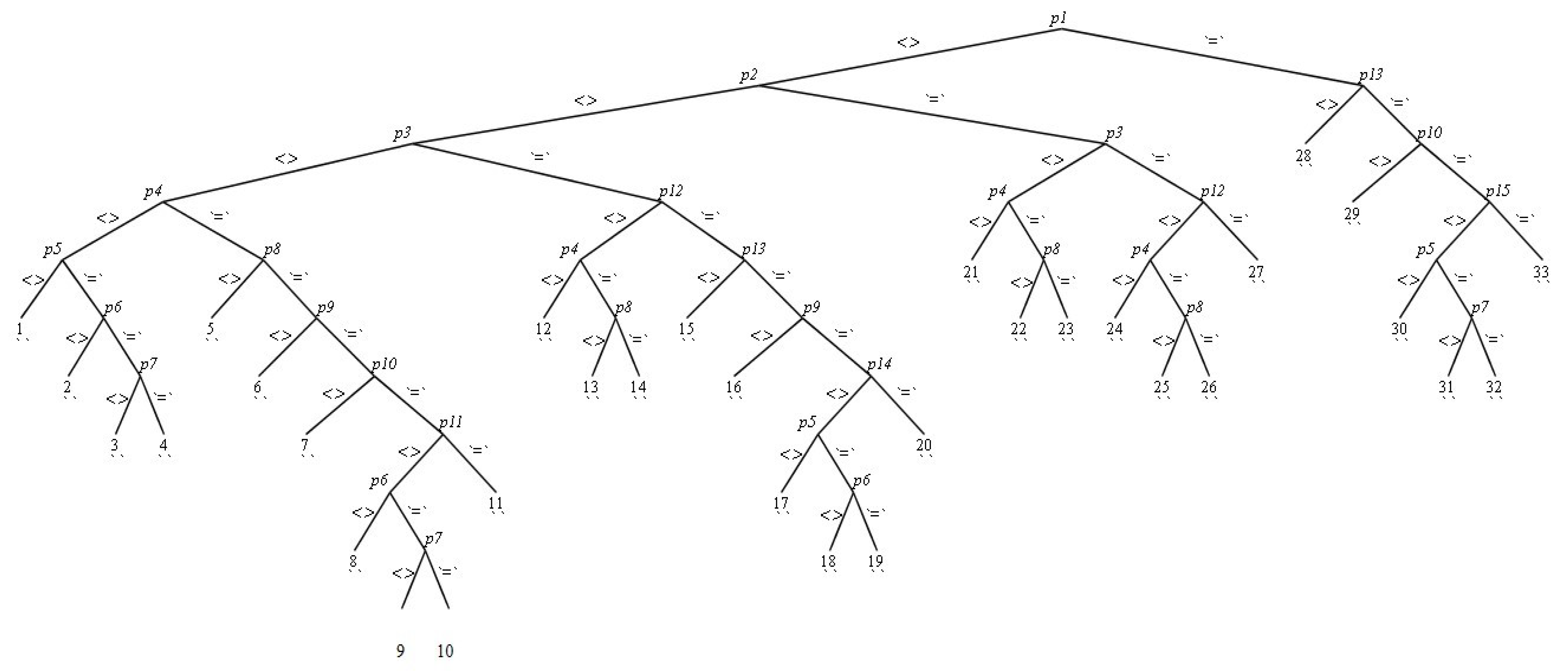
2. Noether Symmetry Equations and the Rif Tree

The general static cylindrically symmetric metric can be written in the form [1]:

$$d{s}^2=-A^{2}d{t}^2+d{r}^2+B^{2}d{\theta }^2+C^{2}d{z}^2,$$

(5)

with three minimum KVFs given by $V_{\left(1\right)}={\partial }_t,V_{\left(2\right)}={\partial }_{\theta }$ and $V_{\left(3\right)}={\partial }_z.$ Out of these three KVFs, $V_{\left(1\right)}$ gives the energy conservation, while $V_{\left(2\right)}$ and $V_{\left(3\right)}$ correspond to linear momenta in two spatial directions. In the above metric, A, B and C depend on r only and are non-zero. Moreover, if any two of these coefficients are same, the above metric becomes static plane symmetric metric possessing an additional rotational KVF. However, we restrict our study to only the case when $A\ne B\ne C.$ Below is the Lagrangian associated with the metric (5).

$$L=-A^2{\dot{t}}^2+{\dot{r}}^2+B^2{\dot{\theta }}^2+C^2{\dot{z}}^2,$$

(6)

and the corresponding geodesic equations are:

$$\begin{array}{ccc}\hfill \ddot{t}& =& 0,\hfill \\ \hfill \ddot{x}-A{A}^{\prime }{\dot{t}}^2-B{B}^{\prime }{\dot{y}}^2-C{C}^{\prime }{\dot{z}}^2& =& 0,\hfill \\ \hfill B\ddot{y}+B^{\prime }\dot{x}\dot{y}& =& 0,\hfill \\ \hfill C\ddot{z}+C^{\prime }\dot{x}\dot{z}& =& 0.\hfill \end{array}$$

(7)

We use the Lagrangian given in Equation (6) in Equation (3) to obtain the following Noether symmetry equations:

$$\begin{array}{ccc}\hfill {\xi }_{,t}={\xi }_{,r}={\xi }_{,\theta }={\xi }_{,z}=F_{,s}& =& 0,\hfill \end{array}$$

(8)

$$\begin{array}{ccc}\hfill 2A^{\prime }{V}^1+2A{V}_{,t}^0& =& A{\xi }_s,\hfill \end{array}$$

(9)

$$\begin{array}{ccc}\hfill 2B^{\prime }{V}^1+2B{V}_{,\theta }^2& =& B{\xi }_s,\hfill \end{array}$$

(10)

$$\begin{array}{ccc}\hfill 2C^{\prime }{V}^1+2C{V}_{,z}^3& =& C{\xi }_s,\hfill \end{array}$$

(11)

$$\begin{array}{ccc}\hfill 2V_{,1}^1& =& {\xi }_s,\hfill \end{array}$$

(12)

$$\begin{array}{ccc}\hfill A^2{V}_{,r}^0-V_{,t}^1& =& 0,\hfill \end{array}$$

(13)

$$\begin{array}{ccc}\hfill A^2{V}_{,\theta }^0-B^2{V}_{,t}^2& =& 0,\hfill \end{array}$$

(14)

$$\begin{array}{ccc}\hfill A^2{V}_{,z}^0-C^2{V}_{,t}^3& =& 0,\hfill \end{array}$$

(15)

$$\begin{array}{ccc}\hfill V_{,\theta }^1+B^2{V}_{,r}^2& =& 0,\hfill \end{array}$$

(16)

$$\begin{array}{ccc}\hfill V_{,z}^1+C^2{V}_{,r}^3& =& 0,\hfill \end{array}$$

(17)

$$\begin{array}{ccc}\hfill B^2{V}_{,z}^2+C^2{V}_{,\theta }^3& =& 0,\hfill \end{array}$$

(18)

$$\begin{array}{ccc}\hfill 2A^2{V}_{,s}^0& =& -F_t,\hfill \end{array}$$

(19)

$$\begin{array}{ccc}\hfill 2V_{,s}^1& =& F_r,\hfill \end{array}$$

(20)

$$\begin{array}{ccc}\hfill 2B^2{V}_{,s}^2& =& F_{\theta },\hfill \end{array}$$

(21)

$$\begin{array}{ccc}\hfill 2C^2{V}_{,s}^3& =& F_z.\hfill \end{array}$$

(22)

The solution of these equations give the explicit form of Noether symmetry vector field $V.$ However, because of their non-linearity, these equations cannot be solved generally unless some conditions are imposed on the metric coefficients $A,B$ and $C.$ In almost all the references cited in the introduction, the Noether symmetry equations were solved by using such restrictions on metric functions and then integrating these equations under these restrictions. The disadvantage of this method is that one do not get a complete list of metrics possessing different Noether algebras. Moreover, the direct integration of Noether symmetry equations is quite cumbersome. Instead of this, here we adopt a new approach by first analyzing these equations by a Maple algorithm (Rif algorithm) which provides a list of all metrics admitting different dimensional Noether algebras. This list of metrics is obtained by imposing some constraints satisfied by $A,B$ and C in the form of a tree, known as Rif tree. After that, we solve the Noether symmetry equations for all these metrics to obtain a complete classification of the mentioned spacetimes. For the above set of equations, we have obtained the Rif tree given in Figure 1. The expressions for the nodes $p1,p2,\dots ,p15$ are given below:

$$\begin{array}{ccc}\hfill p1& =& C^{\prime },p2=C^{″},p3=A^{″},p4=B^{″},p5=B{B}^{″}-{B\prime }^2,p6=C{C}^{″}-{C\prime }^2,\hfill \\ \hfill p7& =& A{A}^{″}-{A\prime }^2,p8=B^{\prime },p9=C{C}^{″\prime }-C^{\prime }{C}^{″},p10=A{A}^{″\prime }-A^{\prime }{A}^{″},\hfill \\ \hfill p11& =& A^{″}C-A^{\prime }{C}^{\prime },p12=A^{\prime },p13=B{B}^{″\prime }-B^{\prime }{B}^{″},p14=C^{″}B-B^{\prime }{C}^{\prime },\hfill \\ \hfill p15& =& B{A}^{″}-B^{\prime }{A}^{\prime }.\hfill \end{array}$$

The branches of the Rif tree give rise to different conditions on the functions $A,B$ and $C.$ For example, for the first branch, labeled by 1, we have $pi\ne 0,$ for $i=1,\dots ,5.$ Equivalently, $C^{\prime }\ne 0,$$C^{″}\ne 0,$$A^{″}\ne 0,$$B^{″}\ne 0$ and $B{B}^{″}-B^{\prime 2}\ne 0.$ Thus, all static cylindrically symmetric metrics satisfying these constraints belong to branch 1 and one need to solve Equations (8)–(22) under these conditions on $A,B$ and C to find all such metrics and their associated Noether symmetries. Similarly, all other branches give different conditions on metric coefficients, and the solutions of Equations (8)–(22) under these conditions give a different list of static cylindrically symmetric metrics and their Noether symmetries. After solving the determining equations for all the 33 branches of the Rif tree, we have concluded that static cylindrically symmetric spacetimes posses Noether algebras of dimensions 4, 5, 6 and 9. We summarize our results in the forthcoming sections.

3. Four Noether Symmetries

Some branches of the Rif tree give rise to metrics possessing only four Noether symmetries. These four Noether symmetries include the three minimum KVFs along with a trivial Noether symmetry $V_{\left(0\right)}={\partial }_s.$ These four symmetries are obtained in branches 2, 3, 13, 22, 24 and 25. The conserved quantities corresponding to these four symmetries $V_{\left(0\right)},\dots ,V_{\left(3\right)}$ are, respectively, obtained as:

$$\begin{array}{ccc}\hfill I_0& =& A^2{\dot{t}}^2-{\dot{r}}^2-B^2{\dot{\theta }}^2-C^2{\dot{z}}^2,\hfill \\ \hfill I_1& =& -2A^2\dot{t},\hfill \\ \hfill I_2& =& 2B^2\dot{\theta },\hfill \\ \hfill I_3& =& 2C^2\dot{z}.\hfill \end{array}$$

4. Five Noether Symmetries

There are many metrics, obtained while using the conditions of different branches to solve Equations (8)–(22), that possess five Noether symmetries. Four of these five symmetries are same as the minimum four Noether symmetries, while the additional symmetry for all metrics is denoted by $V_{\left(4\right)}$ in

Table 1. Metrics with five Noether symmetries.

No/Branch	Metric	Additional Symmetry and Gauge Function	Conserved Quantity
5a	$A={(a_{1}r+2a_3)}^{1-2\frac{a_5}{a_1}},$$B={(a_{1}r+2a_3)}^{1-2\frac{a_7}{a_1}},$	$V_{\left(4\right)}=s{\partial }_s+\frac{r}{2}{\partial }_r$	$I_4=-sL$
1	$C={(a_{1}r+2a_3)}^{1-2\frac{a_9}{a_1}}.$
	where $a_1,a_5,a_7,a_9\ne ,0$ $a_5\ne a_7\ne a_9$
	and $a_1\ne 2a_i,$ for $i=5,7,9$
5b	$A=a_1{e}^{a_{2}r},$$B=a_3{e}^{a_{4}r},$$C=a_5{e}^{a_{6}r},$	$V_{\left(4\right)}=-a_{2}t{\partial }_t+{\partial }_r$	$I_4=2A^2\dot{t}t{a}_2+2\dot{r}$
4	where $a_2\ne a_4\ne a_6$ and $a_i\ne 0,$ for $i=1,\dots ,6.$	$-a_4\theta {\partial }_{\theta }-a_{6}z{\partial }_z.$	$-2B^2\dot{\theta }\theta a_4-2\dot{z}z{C}^2{a}_6.$
5c	$A=B^{a_3},B=a_{1}r+a_2,C=B^{a_4},$	$V_{\left(4\right)}=s{\partial }_s+\frac{t}{2}(1-a_3){\partial }_t$	$I_4=-sL-\dot{t}t{A}^2(1-a_3)$
5	where $a_3\ne 0,1;$ $a_4\ne 0,1;$
	$a_1\ne 0$ and $a_3\ne a_4$	$+\frac{B}{2a_1}{\partial }_r+\frac{z}{2}(1-a_4){\partial }_z,$	$+\dot{r}\frac{B}{a_1}+\dot{z}z{C}^2(1-a_4)$
5d	$A=a_1{e}^{a_{2}r}+a_3{e}^{-a_{2}r},;B=const=\kappa ;$	$V_{\left(4\right)}=\frac{s}{2{\kappa }^2}{\partial }_{\theta }$, $F=\theta$	$I_4=\dot{\theta }s-\theta$
6	$C=C\left(r\right),C\stackrel{⃛}{C}-\dot{C}\ddot{C}\ne 0$ where $a_1,a_2,a_3\ne 0,$
5e	$A=A\left(r\right),A\stackrel{⃛}{A}-\dot{A}\ddot{A}\ne 0;B=const=\kappa ;$	$V_{\left(4\right)}=\frac{s}{2{\kappa }^2}{\partial }_{\theta }$, $F=\theta$	$I_4=\dot{\theta }s-\theta$
7	$C=a_1{e}^{a_{2}r}+a_3{e}^{-a_{2}r}$ where $a_1,a_2,a_3\ne 0,$
5f	$A=a_1{e}^{a_{2}r}+a_3{e}^{-a_{2}r};B=const=\kappa ;$	$V_{\left(4\right)}=\frac{s}{2{\kappa }^2}{\partial }_{\theta }$, $F=\theta$	$I_4=\dot{\theta }s-\theta$
8	$C=a_4{e}^{a_{5}r}+a_6{e}^{-a_{5}r}$ where $a_2,a_4,a_5,a_6\ne 0,$
5g	$A=a_1{e}^{a_{2}r}+a_3{e}^{-a_{2}r};B=const=\kappa ;$	$V_{\left(4\right)}=\frac{s}{2{\kappa }^2}{\partial }_{\theta }$, $F=\theta$	$I_4=\dot{\theta }s-\theta$
9	$C=a_4{e}^{a_{5}r}$ where $a_1,a_2,a_3,a_4,a_5\ne 0,$
5h	$A=a_{1}r+a_2,$$B=A^{a_3}$	$V_{\left(4\right)}=s{\partial }_s+\frac{A}{2a_1}{\partial }_r$	$I_4=A^{2}s{\dot{t}}^2+\frac{A}{a_1}\dot{r}-s{\dot{r}}^2$
12	$C=A^{a_4},$	$+\frac{\theta }{2}(1-a_3){\partial }_{\theta }+\frac{z}{2}(1-a_4){\partial }_z$,	$+\theta \dot{\theta }{B}^2(1-a_3)-s{\dot{\theta }}^2{B}^2$
	where $a_1\ne 0$ $a_i\ne 0,1$ for $i=3,4$		$+\dot{z}z{C}^2(1-a_4)-s{\dot{z}}^2{C}^2$
5i	$A=const=\kappa ,B=a_1{e}^{a_{2}r}+a_3{e}^{-a_{2}r}$	$V_{\left(4\right)}=-\frac{s}{2{\kappa }^2}{\partial }_t$, $F=t$	$I_4=\dot{t}s-t$
16	$C=C\left(r\right),C\stackrel{⃛}{C}-\dot{C}\ddot{C}\ne 0$
	where $a_1,a_2,a_3\ne 0,$
5j	$A=const=\kappa ,B=a_1{e}^{a_{2}r}+a_3{e}^{-a_{2}r}$	$V_{\left(4\right)}=-\frac{s}{2{\kappa }^2}{\partial }_t$, $F=t,$	$I_4=\dot{t}s-t$
17	$C=a_4{e}^{a_{5}r}+a_6{e}^{-a_{5}r}$
	where $a_1,a_2,a_3\ne 0,$
5k	$A=const=\kappa ,B=a_{1}r+a_2$	$V_{\left(4\right)}=-\frac{s}{2{\kappa }^2}{\partial }_t$, $F=t$	$I_4=\dot{t}s-t$
17	$C=a_4{e}^{a_{3}r}+a_5{e}^{-a_{3}r}$
	where $a_1,a_2,a_3\ne 0,$
5l	$A=const=\kappa ,B=a_1{e}^{a_{2}r}$	$V_{\left(4\right)}=-\frac{s}{2{\kappa }^2}{\partial }_t$, $F=t$	$I_4=\dot{t}s-t$
18	$C=a_3{e}^{a_{4}r}+a_5{e}^{-a_{4}r}$
	where $a_1,a_2,a_3,a_4\ne 0,$

and

Table 2. Metrics with five Noether symmetries.

No/Branch	Metric	Additional Symmetry and Gauge Function	Conserved Quantity
5m	$A=C^{a_4},$$B=C^{a_3},$	$V_{\left(4\right)}=s{\partial }_s+\frac{t}{2}(1-a_4){\partial }_t$	$I_4=-\dot{t}t{A}^2(1-a_4)+A^{2}s{\dot{t}}^2$
21	$C=a_{1}r+a_2,$	$+\frac{C}{2a_1}{\partial }_r+\frac{\theta }{2}(1-a_3){\partial }_{\theta }$,	$+\dot{r}\frac{C}{a_1}-s{\dot{r}}^2+\dot{\theta }\theta B^2(1-a_3)$
	where $a_1\ne 0$ and $a_i\ne 0,1$ for $i=3,4$		$-s{B}^2{\dot{\theta }}^2-s{C}^2{\dot{z}}^2$
5n	$A=a_{1}r+a_2,$$B=const=\kappa ,$	$V_{\left(4\right)}=\frac{s}{2{\kappa }^2}{\partial }_{\theta }$, $F=\theta$	$I_4=\dot{\theta }s-\theta$
26	$C=a_{3}r+a_4,$
	where $a_i\ne 0,$ for $i=1,3$
5o	$A=a_1{e}^{a_{2}r}+a_3{e}^{-a_{2}r},$	$V_{\left(4\right)}=\frac{s}{2{\kappa }^2}{\partial }_z$, $F=z$	$I_4=\dot{z}s-z$
28	$B=B\left(r\right),B\stackrel{⃛}{B}-\ddot{B}\dot{B}\ne 0$, $C=const=\kappa ,$
5p	$A=A\left(r\right),A\stackrel{⃛}{A}-\ddot{A}\dot{A}\ne 0,$	$V_{\left(4\right)}=\frac{s}{2{\kappa }^2}{\partial }_z$, $F=z$	$I_4=\dot{z}s-z$
29	$B=a_1{e}^{a_{2}r}+a_3{e}^{-a_{2}r}$, $C=const=\kappa ,$
5q	$A=a_1{e}^{a_{2}r}+a_3{e}^{-a_{2}r},$	$V_{\left(4\right)}=\frac{s}{2{\kappa }^2}{\partial }_z$, $F=z$	$I_4=\dot{z}s-z$
30	$B=a_4{e}^{a_{5}r}+a_6{e}^{-a_{5}r}$, $C=const=\kappa ,$
	where $a_i\ne 0$ for $i=2,4,5,6$
5r	$A=a_1{e}^{a_{2}r}+a_3{e}^{-a_{2}r},$	$V_{\left(4\right)}=\frac{s}{2{\kappa }^2}{\partial }_z$, $F=z$	$I_4=\dot{z}s-z$
30	$B=a_{4}r+a_5$, $C=const=\kappa ,$
	where $a_i\ne 0$ for $i=1,2,3,4,5$
5s	$A=a_{1}r+a_2,$	$V_{\left(4\right)}=\frac{s}{2{\kappa }^2}{\partial }_z$, $F=z$	$I_4=\dot{z}s-z$
30	$B=a_3{e}^{a_{4}r}+a_5{e}^{-a_{4}r}$, $C=const=\kappa ,$
	where $a_i\ne 0$ for $i=1,2,3,4,5$
5t	$A=a_{1}r+a_2,$	$V_{\left(4\right)}=\frac{s}{2{\kappa }^2}{\partial }_z$, $F=z$	$I_4=\dot{z}s-z$
30	$B=a_{3}r+a_4$, $C=const=\kappa ,$
	where $a_i\ne 0$ for $i=1,2,3,4,$
5u	$A=a_1{e}^{a_{2}r}+a_3{e}^{-a_{2}r},$	$V_{\left(4\right)}=\frac{s}{2{\kappa }^2}{\partial }_z$, $F=z$	$I_4=\dot{z}s-z$
31	$B=a_4{e}^{a_{5}r}$, $C=const=\kappa ,$
	where $a_i\ne 0$ for $i=1,2,3,4,5$
5v	$A=a_{1}r+a_2,$	$V_{\left(4\right)}=\frac{s}{2{\kappa }^2}{\partial }_z$, $F=z$	$I_4=\dot{z}s-z$
31	$B=a_3{e}^{a_{4}r}$, $C=const=\kappa ,$
	where $a_i\ne 0$ for $i=1,2,3,4$

, where we list all the obtained metrics along with the explicit form of the additional symmetry and the conserved quantity. For the metrics where $V_{\left(4\right)}$ is independent of $s,$ it denotes a KVF. In case $V_{\left(4\right)}$ is of the form $s\partial s+X,$ it gives rise to a homothetic vector field $X.$ In all other cases, $V_{\left(4\right)}$ gives a proper Noether symmetry.

In a recent study about HVFs of the same spacetime, it was observed that there are many static cylindrically symmetric metrics admitting four HVFs, including three minimum KVFs and one proper HVF [19]. Out of these metrics, four are same as the metrics 5a, 5c, 5h and 5m obtained during our classification. These are the metrics for which $V_{\left(4\right)}$ is of the form $s\partial s+X,$ where X is the HVF that is exactly same as obtained in Ref. [19].

To add some discussion about the singularity of the obtained metrics, we find their corresponding Kretschmann scalar. It is a quadratic scalar invariant, denoted by K and it is defined as $K=R_{abcd}{R}^{abcd};$$R_{abcd}$ being the Riemann tensor. Note that the repeated indices $a,b,c$ and d indicate summation over these indices. For the metric 5a, the value of K is obtained as:

$$\begin{array}{ccc}\hfill K& =& \frac{4}{(a_{1}r+2a_3{)}^4}[4a_5^2{(a_1-2a_5)}^2+4a_7^2{(a_1-2a_7)}^2+4a_9^2{(a_1-2a_9)}^2\hfill \\ & +& {(a_1-2a_5)}^2{(a_1-2a_7)}^2+{(a_1-2a_5)}^2{(a_1-2a_9)}^2+{(a_1-2a_7)}^2{(a_1-2a_9)}^2]\hfill \end{array}$$

(23)

As the term $a_{1}r+2a_3$ is involved in the values of the metric functions $A,B$ and $C,$ thus it is non-zero. Therefore, K is finite and the spacetime has no singularity. Additionally, K is always non-zero because $a_1\ne 2a_5\ne 2a_7\ne 2a_9.$

For the metric 5b, the value of K is found to be:

$$K=4\left[a_2^4+a_4^4+a_6^4+a_2^2{a}_4^2+a_4^2{a}_6^2+a_2^2{a}_6^2\right].$$

(24)

One can see that this value of K is always finite and positive, showing that the metric 5b has no singularity. For metric 5c, the Kretschmann scalar is obtained as:

$$\begin{array}{c}\hfill K=\frac{4a_1^4}{(a_{1}r+a_2{)}^4}\left[a_3^2+a_4^2+a_3^2{a}_4^2+a_3^2{(a_3-1)}^2+a_4^2{(a_4-1)}^2\right],\end{array}$$

(25)

which is again finite as $a_{1}r+a_2\ne 0,$ otherwise, $A,B$ and C vanish. Thus, this metric is also regular. One can see that for the metrics 5h and 5m, the Kretschmann scalar K has a similar structure to that metric 5c. Thus, these metrics are also regular.

For metric 5d, the Kretschmann scalar becomes:

$$\begin{array}{c}\hfill K=\frac{4}{C^2}[{C″}^2+a_2^4{C}^2+\frac{{A\prime }^2{C\prime }^2}{A^2}]\end{array}$$

(26)

As $A\ne 0$ and $C\ne 0,$ therefore the above value of K is always finite, giving a regular metric. Similarly, the metrics 5e, 5f, 5g, 5i, 5j, 5l, 5o, 5p, 5q and 5u are also regular because the Kretschmann scalar for these metrics is similar to that of the metric 5d.

For the metrics 5k, 5r, 5s and 5v, the Kretschmann scalar has a similar structure. Out of these, the Kretschmann scalar K for metric 5k turned out to be:

$$\begin{array}{c}\hfill K=4[a_3^2+\frac{a_1^2{C\prime }^2}{B^2{C}^2}],\end{array}$$

(27)

which is finite because $B\ne 0$ and $C\ne 0.$ Hence, all the metrics 5k, 5r, 5s, and 5v are regular.

The value of the Kretschmann scalar for the metrics 5n and 5t is the same in structure as is obtained as:

$$\begin{array}{c}\hfill K=\frac{4a_1^2{a}_3^2}{A^2{C}^2},\end{array}$$

(28)

which is finite because $A\ne 0$ and $C\ne 0.$ Thus, the metrics 5n and 5t are also regular. Hence all the metrics of this section are regular at every point.

5. Six Noether Symmetries

Like the case of five Noether symmetries, there are many branches of the Rif tree, which give rise to the metrics admitting two additional symmetries along with the four minimum Noether symmetries. These two extra symmetries (denoted by $V_{\left(4\right)}$ and $V_{\left(5\right)}$), their associated conserved quantities and the explicit form of the metrics are listed in

Table 3. Metrics with six Noether symmetries.

No/Branch No	Metric	Additional Symmetries and Gauge Function	Conserved Quantities
6a	$A={(a_{1}r+2a_2)}^{1-\frac{2a_6}{a_1}},$$B=Const.=\kappa ,$	$V_{\left(4\right)}=s{\partial }_s+\frac{r}{2}{\partial }_r+\frac{\theta }{2}{\partial }_{\theta }$,	$I_4=s{A}^2{\dot{t}}^2+r\dot{r}-2s{\dot{r}}^2$
6	$C={(a_{1}r+2a_2)}^{1-\frac{2a_8}{a_1}},$ where $a_1,a_6,a_8\ne 0,$	$V_{\left(5\right)}=\frac{s}{2{\kappa }^2}{\partial }_{\theta }$$F=\theta$	$+\theta \dot{\theta }{B}^2-s{\dot{\theta }}^2{B}^2-s{C}^2{\dot{z}}^2$
	$a_6\ne a_8$ and $a_1\ne 2a_i,$ for $i=6,8.$		$I_5=\dot{\theta }s-\theta$
6b	$A=a_1{e}^{a_{2}r},$$B=const,=\kappa ,$$C=a_3{e}^{a_{4}r},$	$V_{\left(4\right)}=-a_{2}t{\partial }_t+{\partial }_r-a_{4}z{\partial }_z,$	$I_4=2a_2\dot{t}t{A}^2+2\dot{r}-2a_{4}z\dot{z}{C}^2$
10	where $a_1,a_2,a_3,a_4\ne 0$ and $a_2\ne a_4$	$V_{\left(5\right)}=\frac{s}{2{\kappa }^2}{\partial }_{\theta }$, $F=\theta ,$	$I_5=s\dot{\theta }-\theta$
6c	$A=a_{1}r+a_2,$$B=cost=\kappa ,$$C=A^{1-\frac{2a_3}{a_4}},$	$V_{\left(4\right)}=s{\partial }_s+\frac{A}{2a_1}{\partial }_r+\frac{\theta }{2}{\partial }_{\theta }$,	$I_4=s{A}^2{\dot{t}}^2+\frac{A}{a_1}\dot{r}-s{\dot{r}}^2$
14	where $a_1,a_3,a_4\ne 0$ and $a_4\ne 2a_3.$	$V_{\left(5\right)}=\frac{s}{2{\kappa }^2}{\partial }_{\theta },$$F=\theta$,	$+B^2\theta \dot{\theta }-s{B}^2{\dot{\theta }}^2-s{C}^2{\dot{z}}^2$
			$I_5=s\dot{\theta }-\theta$
6d	$A=const.=\kappa ,$$B={(a_{1}r+2a_5)}^{1-\frac{2a_7}{a_1}},$	$V_{\left(4\right)}=s{\partial }_s+\frac{t}{2}{\partial }_t+\frac{r}{2}{\partial }_r$,	$I_4=2A^2(s\dot{t}-t)$
15	$C={(a_{1}r+2a_5)}^{1-\frac{2a_9}{a_1}},$ where $a_1,a_7,a_9\ne 0,$	$V_{\left(5\right)}=-\frac{s}{2{\kappa }^2}{\partial }_t,$$F=t$	$I_5=-A^{2}t\dot{t}+s{A}^2{\dot{t}}^2+r\dot{r}$
	$a_7\ne a_9$ and $a_1\ne 2a_i,$ for $i=7,9.$		$-s{\dot{r}}^2-s{B}^2{\dot{\theta }}^2-s{C}^2{\dot{z}}^2$
6e	$A=cost=\kappa ,$$B=a_{1}r+a_2,$$C=B^{1-\frac{2a_3}{a_4}},$	$V_{\left(4\right)}=s{\partial }_s+\frac{t}{2}{\partial }_t+\frac{B}{2a_1}{\partial }_r$,	$I_4=-A^{2}t\dot{t}+s{A}^2{\dot{t}}^2+\frac{B}{a_1}\dot{r}$
16	where $a_1,a_3,a_4\ne 0$ and $a_4\ne 2a_3.$	$V_{\left(5\right)}=-\frac{s}{2{\kappa }^2}{\partial }_t,$$F=t$,	$-s{\dot{r}}^2-s{B}^2{\dot{\theta }}^2-s{C}^2{\dot{z}}^2$
			$I_5=s\dot{t}-t$
6f	$A=const=\kappa ,$$B=a_1{e}^{a_{2}r},$$C=a_3{e}^{a_{4}r},$	$V_{\left(4\right)}={\partial }_r-a_2\theta {\partial }_{\theta }-a_{4}z{\partial }_z,$	$I_4=2\dot{r}-2a_2{B}^2\theta \dot{\theta }-2a_4{C}^{2}z\dot{z}$
19	where $a_1,a_2,a_3,a_4\ne 0$ and $a_2\ne a_4$	$V_{\left(5\right)}=-\frac{s}{2{\kappa }^2}{\partial }_r,$$F=t$	$I_5=s\dot{t}-t$
6g	$A=C^{1-\frac{2a_3}{a_4}},$$B=cost=\kappa ,$$C=a_{1}r+a_2,$	$V_{\left(4\right)}=s{\partial }_s+\frac{C}{2a_1}{\partial }_r+\frac{\theta }{2}{\partial }_{\theta }$,	$I_4=s{A}^2{\dot{t}}^2+\frac{C}{a_1}\dot{r}-s{\dot{r}}^2$
23	where $a_1,a_3,a_4\ne 0$ and $a_4\ne 2a_3.$	$V_{\left(5\right)}=\frac{s}{2{\kappa }^2}{\partial }_{\theta },$$F=\theta$,	$+B^2\theta \dot{\theta }-s{B}^2{\dot{\theta }}^2-s{C}^2{\dot{z}}^2$
			$I_5=s\dot{\theta }-\theta$
6h	$A=cost=\kappa ,$$B=C^{1-\frac{2a_3}{a_4}},$$C=a_{1}r+a_2,$	$V_{\left(4\right)}=s{\partial }_s+\frac{C}{2a_1}{\partial }_r+\frac{t}{2}{\partial }_t$,	$I_4=-A^{2}t\dot{t}+s{A}^2{\dot{t}}^2+\frac{C}{a_1}\dot{r}$
27	where $a_1,a_3,a_4\ne 0$ and $a_4\ne 2a_3.$	$V_{\left(5\right)}=-\frac{s}{2{\kappa }^2}{\partial }_t,$$F=t$	$-s{\dot{r}}^2-s{B}^2{\dot{\theta }}^2-s{C}^2{\dot{z}}^2$
			$I_5=s\dot{t}-t$
6i	$A={(a_{1}r+2a_2)}^{1-\frac{2a_6}{a_1}},$$B={(a_{1}r+2a_2)}^{1-\frac{2a_8}{a_1}},$	$V_{\left(4\right)}=s{\partial }_s+\frac{r}{2}{\partial }_r+\frac{z}{2}{\partial }_z$,	$I_4=s{A}^2{\dot{t}}^2+r\dot{r}-s{\dot{r}}^2$
28	$C=Const.=\kappa ,$ where $a_1,a_6,a_8\ne 0,$	$V_{\left(5\right)}=\frac{s}{2{\kappa }^2}{\partial }_z,$$F=z$	$-s{\dot{\theta }}^2{B}^2+z{C}^2\dot{z}-s{C}^2{\dot{z}}^2$
	$a_6\ne a_8$ and $a_1\ne 2a_i,$ for $i=6,8.$		$I_5=s\dot{z}-z$
6j	$A=B^{1-\frac{2a_3}{a_4}},$$B=a_{1}r+a_2,$$C=cost=\kappa ,$	$V_{\left(4\right)}=s{\partial }_s+\frac{B}{2a_1}{\partial }_r+\frac{z}{2}{\partial }_z$,	$I_4=s{A}^2{\dot{t}}^2+\frac{B}{a_1}\dot{r}-s{\dot{r}}^2$
29	where $a_1,a_3,a_4\ne 0$ and $a_4\ne 2a_3.$	$V_{\left(5\right)}=\frac{s}{2{\kappa }^2}{\partial }_z,$$F=t$,	$-s{B}^2{\dot{\theta }}^2+C^{2}z\dot{z}-s{C}^2{\dot{z}}^2$
			$I_5=s\dot{z}-z$
6k	$A=a_1{e}^{a_{2}r},$$B=a_3{e}^{a_{4}r},$$C=const.=\kappa ,$	$V_{\left(4\right)}=-a_{2}t{\partial }_t+{\partial }_r-a_4\theta {\partial }_{\theta }$,	$I_4=2a_2{A}^{2}t\dot{t}+2\dot{r}-2a_4{B}^2\theta \dot{\theta }$
32	where $a_1,a_2,a_3\ne 0$ $a_2\ne a_4$	$V_{\left(5\right)}=\frac{s}{2{\kappa }^2}{\partial }_z$	$I_5=s\dot{z}-z$

. For the metrics of branches 10, 19 and 32, $V_{\left(4\right)}$ is a KVF, while for other branches it corresponds to a HVF. In all branches, $V_{\left(5\right)}$ is a proper Noether symmetry.

For the metrics 6a, 6c, 6d, 6e, 6g, 6h, 6i and 6j, $V_{\left(4\right)}$ is of the form $s\partial s+X,$ where X is the HVF admitted by the corresponding metric and for all these eight metrics, this HVF is same as obtained in Ref. [19].

To check the singularity of the metric 6a, we find its Kretschmann scalar given by:

$$\begin{array}{c}\hfill K=\frac{4}{(a_{1}r+2a_2{)}^4}[4a_6^2{(a_1-2a_6)}^2+4a_8^2{(a_1-2a_8)}^2+{(a_1-2a_6)}^2{(a_1-2a_8)}^2],\end{array}$$

(29)

which is finite as $a_{1}r+2a_2\ne 0.$ It shows that this metric has no singularity. For the metrics 6d and 6i, K has a similar structure, showing that these metrics are also regular. For metric 6b, K receives the value:

$$K=4\left[a_2^4+a_4^4+a_2^2{a}_4^2\right],$$

(30)

which is clearly finite, showing that the metric has no singularity. Similarly, 6f and 6k, being similar to 6b, are also regular metrics.

The value of K for the metrics 6c, 6e, 6g, 6h, and 6j has a similar structure. Out of these, the Kretschmann scalar for the metric 6c is found to be:

$$\begin{array}{c}\hfill K=\frac{16a_1^2{(2a_3-a_4)}^2(4a_3^2+a_4^2)}{a_4^4{(a_{1}r+a_2)}^4},\end{array}$$

(31)

which is finite because $a_{1}r+a_2\ne 0$ and $a_4\ne 0.$ Hence, the metrics 6c, 6e, 6g, 6h and 6j have no singularity.

6. Nine Noether Symmetries

Three branches labeled by 11, 20 and 33 produce metrics possessing five additional symmetries along with the four minimum Noether symmetries. For each metric, we have obtained four additional KVFs, represented by $V_{\left(4\right)},\dots ,V_{\left(7\right)}$ and one proper Noether symmetry, denoted by $V_{\left(8\right)}$ in

Table 4. Metrics with nine Noether symmetries.

No/Branch	Metric	Additional Symmetries	Conserved Quantities
9a	$A=a_2{e}^{a_{1}r}+a_3{e}^{-a_{1}r},$	$V_{\left(4\right)}=sin\left(mz\right)cos\left(nt\right)\frac{A^{\prime }}{nA}{\partial }_t+sin\left(mz\right)sin\left(nt\right){\partial }_r$	$I_4=-2\frac{A{A}^{\prime }}{n}\dot{t}sin\left(mz\right)cos\left(nt\right)+2\dot{r}sin\left(mz\right)sin\left(nt\right)$
11		$+cos\left(mz\right)sin\left(nt\right)\frac{A{a}_4}{mC}{\partial }_z.$	$+2\frac{a_{4}CA}{m}\dot{z}cos\left(mz\right)sin\left(nt\right)$
	$B=const=\kappa ,$	$V_{\left(5\right)}=cos\left(mz\right)cos\left(nt\right)\frac{A^{\prime }}{nA}{\partial }_t+cos\left(mz\right)sin\left(nt\right){\partial }_r$	$I_5=-2\frac{A{A}^{\prime }}{n}\dot{t}cos\left(mz\right)cos\left(nt\right)+2\dot{r}cos\left(mz\right)sin\left(nt\right)$
		$-sin\left(mz\right)sin\left(nt\right)\frac{A{a}_4}{mC}{\partial }_z$	$-2\frac{a_{4}CA}{m}\dot{z}sin\left(mz\right)sin\left(nt\right)$
	$C=\frac{a_4}{a_1}(a_2{e}^{a_{1}r}-a_3{e}^{-a_{1}r})$	$V_{\left(6\right)}=-sin\left(mz\right)sin\left(nt\right)\frac{A^{\prime }}{nA}{\partial }_t+sin\left(mz\right)cos\left(nt\right){\partial }_r$
		$+cos\left(mz\right)cos\left(nt\right)\frac{A{a}_4}{mC}{\partial }_z$,	$I_6=2\frac{A{A}^{\prime }}{n}\dot{t}sin\left(mz\right)sin\left(nt\right)+2\dot{r}sin\left(mz\right)cos\left(nt\right)$
	where $m=2a_4\sqrt{a_2{a}_3},$		$+2\dot{z}\frac{a_{4}AC}{m}cos\left(mz\right)cos\left(nt\right).$
	$n=2a_1\sqrt{a_2{a}_3}$	$V_{\left(7\right)}=cos\left(mz\right)sin\left(nt\right)\frac{A^{\prime }}{nA}{\partial }_t+cos\left(mz\right)cos\left(nt\right){\partial }_r$	$I_7=2\frac{A{A}^{\prime }}{n}\dot{t}cos\left(mz\right)sin\left(nt\right)+2\dot{r}cos\left(mz\right)cos\left(nt\right)$
		$-sin\left(mz\right)cos\left(nt\right)\frac{A{a}_4}{mC}{\partial }_z,$	$-2\frac{a_{4}CA}{m}\dot{z}sin\left(mz\right)cos\left(nt\right).$
	and $a_1,a_2,a_3,a_4\ne 0$
		$V_{\left(8\right)}=\frac{s}{2{\kappa }^2}{\partial }_{\theta },$$F=\theta$	$I_8=s\dot{\theta }-\theta$
9b	$A=const=\kappa ,$	$V_{\left(4\right)}=sin\left(mz\right)e^{n\theta }{\partial }_r-sin\left(mz\right)e^{n\theta }\frac{B^{\prime }}{nB}{\partial }_{\theta }$	$I_4=2\dot{r}sin\left(mz\right)e^{n\theta }-2\dot{\theta }\frac{B{B}^{\prime }}{n}sin\left(mz\right)e^{n\theta }$
20		$cos\left(mz\right)e^{n\theta }\frac{B{a}_4}{mC}{\partial }_z.$	$+2\frac{a_{4}CB}{m}\dot{z}cos\left(mz\right)e^{n\theta }$
	$B=a_2{e}^{a_{1}r}+a_3{e}^{-a_{1}r},$	$V_{\left(5\right)}=cos\left(mz\right)e^{n\theta }{\partial }_r-cos\left(mz\right)e^{n\theta }\frac{B^{\prime }}{nB}{\partial }_{\theta }$	$I_5=2\dot{r}cos\left(mz\right)e^{n\theta }-2\dot{\theta }cos\left(mz\right)e^{n\theta }\frac{B{B}^{\prime }}{n}$
		$-sin\left(mz\right)e^{n\theta }\frac{B{a}_4}{mC}{\partial }_z$	$-2\frac{a_{4}CB}{m}\dot{z}sin\left(mz\right)e^{n\theta }$
	$C=\frac{a_4}{a_1}(a_2{e}^{a_{1}r}-a_3{e}^{-a_{1}r})$	$V_{\left(6\right)}=sin\left(mz\right)e^{-n\theta }{\partial }_r+sin\left(mz\right)e^{-n\theta }\frac{B^{\prime }}{nB}{\partial }_{\theta }$
		$+cos\left(mz\right)e^{-n\theta }\frac{B{a}_4}{mC}{\partial }_z$,	$I_6=2\dot{r}sin\left(mz\right)e^{-n\theta }+2\dot{\theta }sin\left(mz\right)e^{-n\theta }\frac{B{B}^{\prime }}{n}$
	where $m=2a_4\sqrt{a_2{a}_3},$		$+2\dot{z}\frac{a_{4}BC}{m}cos\left(mz\right)e^{-n\theta }.$
	$n=2a_1\sqrt{a_2{a}_3}$	$V_{\left(7\right)}=cos\left(mz\right)e^{-n\theta }{\partial }_r+cos\left(mz\right)e^{-n\theta }\frac{B^{\prime }}{nB}{\partial }_{\theta }$	$I_7=2\dot{r}cos\left(mz\right)e^{-n\theta }+2\dot{\theta }cos\left(mz\right)e^{-n\theta }\frac{B{B}^{\prime }}{n}$
		$-sin\left(mz\right)e^{-n\theta }\frac{B{a}_4}{mC}{\partial }_z,$	$-2\frac{a_{4}CB}{m}\dot{z}sin\left(mz\right)e^{-n\theta }.$
	and $a_1,a_2,a_3,a_4\ne 0$
		$V_{\left(8\right)}=-\frac{s}{2{\kappa }^2}{\partial }_t,$$F=t$	$I_8=s\dot{t}-t$
9c	$A=a_2{e}^{a_{1}r}+a_3{e}^{-a_{1}r},$	$V_{\left(4\right)}=sin\left(my\right)cos\left(nt\right)\frac{A^{\prime }}{nA}{\partial }_t+sin\left(my\right)sin\left(nt\right){\partial }_r$	$I_4=-2\frac{A{A}^{\prime }}{n}\dot{t}sin\left(my\right)cos\left(nt\right)+2\dot{r}sin\left(my\right)sin\left(nt\right)$
33		$+cos\left(my\right)sin\left(nt\right)\frac{A{a}_4}{mB}{\partial }_z.$	$+2\frac{a_{4}BA}{m}\dot{\theta }cos\left(my\right)sin\left(nt\right)$
	$B=\frac{a_4}{a_1}(a_2{e}^{a_{1}r}-a_3{e}^{-a_{1}r}),$	$V_{\left(5\right)}=cos\left(my\right)cos\left(nt\right)\frac{A^{\prime }}{nA}{\partial }_t+cos\left(my\right)sin\left(nt\right){\partial }_r$	$I_5=-2\frac{A{A}^{\prime }}{n}\dot{t}cos\left(my\right)cos\left(nt\right)+2\dot{r}cos\left(my\right)sin\left(nt\right)$
		$-sin\left(my\right)sin\left(nt\right)\frac{A{a}_4}{mB}{\partial }_z$	$-2\frac{a_{4}BA}{m}\dot{\theta }sin\left(my\right)sin\left(nt\right)$
	$C=const=\kappa$	$V_{\left(6\right)}=-sin\left(my\right)sin\left(nt\right)\frac{A^{\prime }}{nA}{\partial }_t+sin\left(my\right)cos\left(nt\right){\partial }_r$
		$+cos\left(my\right)cos\left(nt\right)\frac{A{a}_4}{mB}{\partial }_z$,	$I_6=2\frac{A{A}^{\prime }}{n}\dot{t}sin\left(my\right)sin\left(nt\right)+2\dot{r}sin\left(my\right)cos\left(nt\right)$
	where $m=2a_4\sqrt{a_2{a}_3},$		$+2\dot{\theta }\frac{a_{4}AB}{m}cos\left(my\right)cos\left(nt\right).$
	$n=2a_1\sqrt{a_2{a}_3}$	$V_{\left(7\right)}=-cos\left(my\right)sin\left(nt\right)\frac{A^{\prime }}{nA}{\partial }_t+cos\left(my\right)cos\left(nt\right){\partial }_r$	$I_7=2\frac{A{A}^{\prime }}{n}\dot{t}cos\left(my\right)sin\left(nt\right)+2\dot{r}cos\left(my\right)cos\left(nt\right)$
		$-sin\left(my\right)cos\left(nt\right)\frac{A{a}_4}{mB}{\partial }_z,$	$-2\frac{a_{4}BA}{m}\dot{\theta }sin\left(my\right)cos\left(nt\right).$
	and $a_1,a_2,a_3,a_4\ne 0$
		$V_{\left(8\right)}=\frac{s}{2{\kappa }^2}{\partial }_{\theta },$$F=\theta$	$I_8=s\dot{\theta }-\theta$

. For all the metrics of this section, the Kretschmann scalar is obtained as $K=12a_1^4,$ which shows that all these metrics are regular.

7. Summary and Discussion

We have achieved a complete classification of static cylindrically symmetric spacetimes via their Noether symmetries. For this purpose, instead of the conventional method, we have used a new approach based on a Maple algorithm, which provided a number of metrics possessing different Noether algebras with dimensions 4, 5, 6 and 9. The expressions for the conserved quantities associated with all the obtained Noether symmetries are found by using Noether’s theorem. The authors of Ref. [20] classified the same spacetime via its Noether symmetries using direct integration technique. Though the algebra of Noether symmetries is obtained the same as in our current investigations, the metrics obtained in our study through the Rif tree approach are more generalized than those given in Ref. [20]. In fact, one may easily recover all the metrics of Ref. [20] by taking specific values of the parameters involved in the obtained metrics of the current classification.

The present classification also provides a complete list of static cylindrically symmetric metrics along with their Killing and homothetic symmetries. The dimension of Killing algebra turned out to be 3, 4 and 7. For the metrics of branches 4, 10, 19 and 32, we have obtained 4-dimensional Killing algebra, while the metrics of branches 11, 20 and 33 admit 7-dimensional Killing algebra. For all other metrics, the Killing algebra is minimum dimensional, that is three-dimensional. Moreover, it can be seen that there are twelve different metrics (four in Section 4 and eight in Section 5) admitting proper HVFs. In all these cases, $V_{\left(4\right)}$ represents a symmetry of the form $2\lambda s{\partial }_s+V$ with the homothety constant $\lambda =\frac{1}{2}.$ As stated in the introduction part, in such a case V represents a proper HVF. This result has been verified by comparing the HVFs obtained during the current classification with those of Ref. [19]. Thus, the present analysis shows that the classification of the Lagrangian associated to a spacetime metric via Noether symmetries also gives a complete classification of the corresponding metric through its Killing and homothetic symmetries.

References

1. Stephani, H.; Kramer, D.; Maccallum, M.; Hoenselaers, C.; Herlt, E. Exact Solutions of Einstein’s Field Equations, 2nd ed.; Cambridge University Press: Cambridge, UK, 2003. [Google Scholar]
2. Hall, G.S. Symmetries and Curvature Structure in General Relativity; World Scientific: London, UK, 2004. [Google Scholar]
3. Maartens, R.; Maharaj, S.D. Conformal symmetries of pp-waves. Class. Quantum Gravity 1991, 8, 503. [Google Scholar] [CrossRef]
4. Moopanar, S.; Maharaj, S.D. Relativistic shear-free fluids with symmetry. Relativistic shear-free fluids with symmetry. J. Eng. Math. 2013, 82, 125–131. [Google Scholar] [CrossRef] [Green Version]
5. Saifullah, K.; Yazdan, S. Conformal motions in plane symmetric static space-times. Int. J. Mod. Phys. D 2009, 18, 71–81. [Google Scholar] [CrossRef]
6. Maartens, R.; Maharaj, S.D.; Tupper, B.O.J. General solution and classification of conformal motions in static spherical spacetimes. Class. Quantum Gravity 1995, 12, 2577. [Google Scholar] [CrossRef]
7. Moopanar, S.; Maharaj, S.D. Conformal Symmetries of Spherical Spacetimes. Int. J. Theor. Phys. 2010, 49, 1878. [Google Scholar] [CrossRef] [Green Version]
8. Khan, S.; Hussain, T.; Bokhari, A.H.; Khan, G.A. Conformal Killing vectors in LRS Bianchi type V spacetimes. Commun. Theor. Phys. 2016, 65, 315. [Google Scholar] [CrossRef]
9. Khan, S.; Hussain, T.; Bokhari, A.H.; Khan, G.A. Conformal Killing vectors of plane symmetric four dimensional Lorentzian manifolds. Eur. Phys. J. C 2015, 75, 523. [Google Scholar] [CrossRef] [Green Version]
10. Hussain, T.; Khan, S.; Bokhari, A.H.; Khan, G.A. Proper conformal Killing vectors in static plane symmetric space-times. Theor. Math. Phys. 2017, 191, 620–629. [Google Scholar] [CrossRef]
11. Hussain, T.; Farhan, M. Proper conformal Killing vectors in Kantowski-Sachs metric. Commun. Theor. Phys. 2018, 69, 393. [Google Scholar] [CrossRef]
12. Noether, E. Invariant variations problems. Transp. Theory Stat. Phys. 1971, 1, 186. [Google Scholar] [CrossRef]
13. Hickman, M.; Yazdan, S. Noether symmetries of Bianchi type II spacetimes. Gen. Relativ. Gravit. 2017, 49, 65. [Google Scholar] [CrossRef]
14. Bokhari, A.H.; Kara, A.H. Noether versus Killing symmetry of conformally flat Friedmann metric. Gen. Relativ. Gravit. 2007, 39, 2053–2059. [Google Scholar] [CrossRef]
15. Bokhari, A.H.; Kara, A.H.; Kashif, A.R.; Zaman, F.D. Noether symmetries versus Killing vectors and isometries of spacetimes. Int. J. Theor. Phys. 2006, 45, 1029–1039. [Google Scholar] [CrossRef]
16. Ali, F.; Feroze, T. Classification of plane symmetric static space-times according to their Noether symmetries. Int. J. Theor. Phys. 2013, 52, 3329–3342. [Google Scholar] [CrossRef]
17. Ali, F.; Feroze, T.; Ali, S. Complete classification of spherically symmetric static space-times via Noether symmetries. Theor. Math. Phys. 2015, 184, 973–985. [Google Scholar] [CrossRef] [Green Version]
18. Ali, S.; Hussain, I. A study of positive energy condition in Bianchi V spacetimes via Noether symmetries. Eur. Phys. J. C 2016, 76, 63. [Google Scholar] [CrossRef] [Green Version]
19. Khan, J.; Hussain, T.; Santina, D.; Mlaiki, N. Homothetic Symmetries of Static Cylindrically Symmetric Spacetimes—A Rif Tree Approach. Axioms 2022, 11, 506. [Google Scholar] [CrossRef]
20. Ali, F.; Feroze, T. Complete classification of cylindrically symmetric static spacetimes and the corresponding conservation laws. Mathematics 2016, 4, 50. [Google Scholar] [CrossRef]
Figure 1. Rif tree.
Symmetry 15 00184 g001