Uncertain Sensor–Weapon–Target Allocation Problem Based on Uncertainty Theory

Abstract

The sensor–weapon–target allocation (S-WTA) is a typical collaborative task allocation problem involved in network-centric warfare (NCW). The existing related studies have a limitation to the nature of cooperation and uncertainty in an air defense battle scenario, and most existing models have the assumption that they are determinate, i.e., the parameters in them are known certainly. For the actual battlefield environment, the asymmetric information in it could lead to the failure of the above assumption, and there are many uncertainties whose frequency can not be evaluated objectively. Based on uncertainty theory, this paper studied the S-WTA problem in an indeterminate battlefield environment. First, we analyze the uncertain factors existing in the actual battlefield environment and their influence on the S-WTA problem, and by considering the threat value of the target, the deviation parameters of the sensor tracking performance and weapon interception performance as uncertain variables, we then establish an uncertain S-WTA (USWTA) model, where the destruction value to targets is regarded as an objective function and four categories of typical constraints are set. Further, an equivalent transformation is presented to convert the unsolvable model into a determinate one by the expected value principle. To solve the proposed model efficiently, a permutation-based representation for the allocation scheme of the USWTA problem is introduced firstly, which can construct a feasible solution efficiently, and on this basis, a constructive heuristic algorithm based on maximum marginal return rule (MMRCH) is designed to construct a feasible solution with high quality. Additionally, a local search (LS) operation is proposed to explore for the better solution locally and further improve the quality of solution obtained by MMRCH. Finally, a set of instances are set to be solved by the designed algorithm, and the simulation experiment demonstrates the superiority of the designed algorithm and the feasibility of the proposed model.

1. Introduction

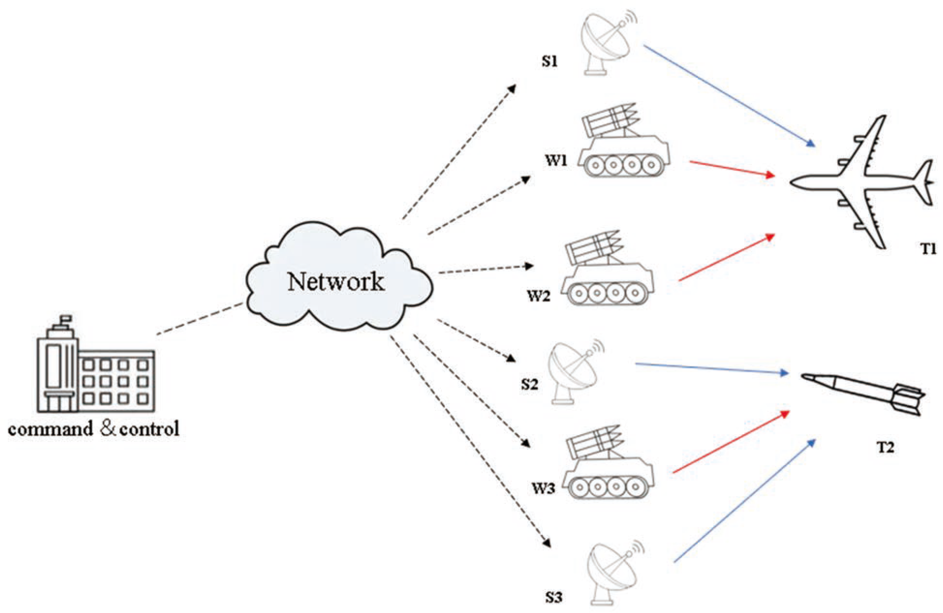
Network-centric warfare (NCW) is becoming a mainstream modern combat style, enabling rapid sharing of information between systems and greatly increasing the speed of the “Observe-Orient-Decide-Act” (OODA) loop proposed by Boyd. From the point of view of the classic OODA loop, the combat system is mainly composed of three categories: sensor platforms, weapon platforms, and command and control (C2) platforms. Specifically, the sensor platforms play the role of “Observer”, which acquire battlefield situation information and provide guidance information for weapon platforms. The C2 platforms play the roles of “Orient” and “Decide”, which process the collected battlefield situation information to make operational decisions. Finally, the weapon platforms play the role of “Act”, which intercept the targets under the command of the C2 platforms and the guidance information provided by sensor platforms. As two major resources in the NCW, the sensor platforms and weapon platforms are organized in a distributed network and can share the information in real time among the network centers. Thus, how to combine these platforms to form effective cooperation and allocate them to targets for engagement to improve combat effectiveness becomes an important research subject.

The problem regarding the allocation of sensors and weapons has been studied since the 1950s, and related studies can be divided into two categories according to the relationship between sensors systems and weapons systems. In the first category, the sensors system and weapons system are independent, and it leads to two types of task allocation problems: the sensor-target allocation (STA) problem [1,2,3,4] and the weapon-target allocation (WTA) problem [5,6,7,8,9,10]. They are considered classical combinatorial optimization problems and have proven to be NP-hard [11]. However, in actual combat, the interception of targets by weapons system requires the real-time guidance from the sensors system; thus, the tracking performance of sensors on the targets has an influence on the interception effectiveness, i.e., the sensors and weapons are not independent of each other, and it is needed to combine sensors and weapons to accomplish task allocation cooperatively, which leads to the sensor–weapon–target allocation (S-WTA) problem. Bogdanowicz [12] was the first to study the S-WTA problem and proposed two types of S-WTA models by analyzing the characteristics of it. Li [13] proposed an improved dependent S-WTA model introduced by the temporal and spatial constraints, which is a kind of dynamic WTA problem. Jian [14] developed an S-WTA model in which the damage probability of a target is influenced by both the destructive capacity of weapons and the tracking capacity of sensors. Xin [15] proposed a novel dependent S-WTA model in which the probability of successful engagement is the product of the interception probability of the weapons and the detection probability of the sensors. Xu [16] proposed a dependent dynamic S-WTA model that has bi-objective and multi-stage considerations, and is also more practical.

For the literature mentioned above, a wide assumption is that the battlefield environment is deterministic and the parameters in the models are known certainly, which neglects the influence of asymmetric information and uncertain factors in the actual situation on task allocation. On one hand, the possible electromagnetic interference and decoys released by the opponent make it difficult to detect the target state information accurately, and the target threat value can not be estimated objectively. Expert reliability is a common method to deal with this uncertainty. On the other hand, due to the unreliability of equipment systems and the maneuverability and stealth capability of targets, the performance of weapon systems and sensor systems in an engagement may deviate from the theoretical value. Therefore, the S-WTA problem is often uncertain with vagueness or imprecision, which is caused by an inaccurate observation of parameters, deficiency in history statistical data, and subjectivity of human judgment. The uncertainty in the S-WTA problem was studied by some scholars. Krokhmal [17] studied the uncertainty of the interception probability using the CVaR constraint. Ahner [18] regarded the number of targets for a subsequent engagement as a random variable, and a two-stage stochastic programming model was proposed. Li [19] proposed a robust optimization model for dealing with the uncertainty in the interception process. Most of the existing studies consider the uncertainty in S-WTA problem as random variables, and then the probability theory is used to deal with them. However, the application of probability theory is based on the law of large numbers [20], i.e., it needs a large scale of historical sample data to support the credibility of results, which is hard to meet in an actual combat scenario due to its unrepeatability. In this case, we can invite experts to estimate the distribution function for each uncertain parameter. Some surveys have shown that human beings usually overestimate the occurrence degree of unlikely events, and the expert belief degree may have larger variance than the real frequency of events; thus, if the probability theory is still used to deal with them, the conclusion may be a paradox [20]. To better describe the subjective imprecise quantity, Liu [21] proposed the uncertainty theory, which is a branch of mathematics based on normality, duality, subadditivity, and product axioms, and it is an effective tool to deal with imprecision rather than randomness. To date, many scholars have studied the uncertainty theory and a complete mathematical system is established, including uncertain set [22], uncertain process [23], uncertain differential equation [24], and two-stage uncertain programming [25,26]. Meanwhile, it has been studied in many application fields, such as uncertain inference [22], uncertain programming [27], uncertain statistics [28], uncertain portfolio selection [29], and uncertain optimal control [30]. So far, there are few relevant studies on the S-WTA problem based on uncertainty theory.

Due to the NP-hard nature of solving the large-scale S-WTA problem, many heuristic algorithms and evolutionary algorithms (EAs) have been designed in the past related studies. In the aspect of EAs, since it can use a flexible evolutionary mechanism to search for satisfactory solutions and usually has high robustness, it has been used to deal with the large scale S-WTA problems. Jian [14] proposed a modified genetic algorithm (GA) to solve a dependent S-WTA model where the kill probability of weapons was affected by the detection performance of sensors. Chen [31] improved the particle swarm optimization (PSO) algorithm with genetic operators and used it to solve an S-WTA model where a target can assign multiple weapons. However, one disadvantage of EAs is that their running time is relatively large. In the aspect of heuristic algorithms, since they can use the domain knowledge of the problem to obtain the solution with high quality, they have been used to solve the S-WTA problem and generally perform well in real-time performance. Bogdanowicz [12] designed a heuristic algorithm named Swt-opt based on the auction algorithm, and it was proved that the algorithm can obtain a complete optimal solution in finite steps, but it can only be applied in scenarios where a target can only be assigned a single sensor and a single weapon. Li [32] combined Swt-opt with the consensus algorithm to enhance the adaptability of Swt-opt to network topologies, but its application scenario is still limited. Xin [15] proposed a marginal-return-based constructive heuristic (MRBCH) to solve a dependent S-WTA model, so as to construct the solution with high quality rapidly and accurately. Xu [16] applied similar heuristic rules in solving a multi-stage S-WTA model, so as to produce a high quality initial population. However, the process of heuristic algorithms is generally fixed, which may traps the solutions into local optimality. In conclusion, the performance of heuristic algorithms and evolutionary algorithms is very sensitive to the parameters involved in it, and they have their own advantages and disadvantages, so how to designed an efficient algorithm combined their advantages to solve scenario-based S-WTA problem with uncertainty is a research key.

The aim of this paper is to solve the S-WTA problem in an indeterminate battlefield environment based on uncertainty theory. First, by analyzing the uncertain factors in the air defense battlefield environment, we treat the threat value of targets, the deviation of the interception performance of weapons and the deviation of the tracking performance of sensors as uncertain variables, then an uncertain S-WTA model (USWTA) is formulated. To make the proposed model solvable, a deterministic model named E-USWTA is derived based on expected value principle. For efficiently solving the proposed model with its NP-hard nature, a virtual representation (VP) and corresponding construction procedure (CP) of a feasible solution for the USWTA problem is introduced firstly, and then on this basis, a heuristic algorithm based on maximum marginal return (MMRCH) is designed to construct a solution with high quality, which utilizes the domain knowledge of the problem to add the allocation pairs to an allocation scheme. Additionally, a local search (LS) operation is employed to avoid missing the better solution in the neighborhood. Finally, a set of instances of the USWTA problem is generated and solved by the designed algorithm, and the allocation schemes with high quality can be obtained. The simulation results verify the effectiveness of the designed algorithm and the feasibility of the proposed model.

The rest of this paper is structured as follows. In Section 2, some basic definitions and theorems of uncertainty theory that are used subsequently are reviewed. In Section 3, the combat scenario is given and the USWTA model is established. In Section 4, the solution method of the USWTA model is derived. In Section 5, the heuristic algorithm based on maximum marginal return with local search is designed for solving the USWTA problems. Section 6 presents a set of instances of the USWTA problem to be solved by the designed algorithm, and the simulation results are analyzed. Finally, the main results of this paper are concluded in Section 7.

2. Preliminaries

Let $\Gamma$ be a nonempty set, and $\mathcal{L}$ is a $\sigma$-algebra over $\Gamma$. Each element $\Lambda$ in $\mathcal{L}$ is called an event. A set function $\mathcal{M}$ from $\mathcal{L}$ to [0,1] is called an uncertain measure if it satisfied the following axioms:

Axiom 1. (Normality Axiom) $\mathcal{M}\{\Gamma \}=1$ for the universal set $\Gamma$;

Axiom 2. (Duality Axiom) $\mathcal{M}\{\Lambda \}+\mathcal{M}\left\{{\Lambda }^c\right\}=1$ for any event $\Lambda \in \mathcal{L}$;

Axiom 3. (Subadditivity Axiom) For any countable sequence of events ${\Lambda }_1,{\Lambda }_2,\dots \in \mathcal{L}$, we have

$$\mathcal{M}\left\{\bigcup _{i=1}^{\infty }{\Lambda }_i\right\}\le \sum _{i=1}^{\infty }\mathcal{M}\left\{{\Lambda }_i\right\}.$$

The triplet $(\Gamma ,\mathcal{L},\mathcal{M})$ is called an uncertainty space. Furthermore, a product axiom of uncertain measure is defined by Liu [21].

Axiom 4. (Product Axiom) Let $({\Gamma }_i,{\mathcal{L}}_i,{\mathcal{M}}_i)$ be the uncertainty space for $i=1,2,\dots$. The product uncertain measure $\mathcal{M}$ is an uncertain measure satisfying

$$\mathcal{M}\left\{\prod _{i=1}^{\infty }{\Lambda }_i\right\}=\underset{i=1}{\overset{\infty }{\bigwedge }}\mathcal{M}\left\{{\Lambda }_i\right\}.$$

Definition 1

([21]). An uncertain variable is a measurable function ξ from an uncertainty space $(\Gamma ,\mathcal{L},\mathcal{M})$ to the set of real numbers, i.e., for any Borel set B of real numbers, the set

$$\left\{\xi \in B\right\}=\left\{\gamma \in \Gamma |\xi \left(\gamma \right)\in B\right\}$$

is an event in $\mathcal{L}$.

Definition 2

([28]). The uncertain variables ${\xi }_1,{\xi }_2,\dots ,{\xi }_n$ are said to be independent if

$$\mathcal{M}\left\{\bigcap _{i=1}^n({\xi }_i\in B_i)\right\}=\underset{i=1}{\overset{n}{\bigwedge }}\mathcal{M}\left\{({\xi }_i\in B_i)\right\}$$

for any Borel sets $B_1,B_2,\dots ,B_n$ of real numbers.

Theorem 1

([28]). The uncertain variables ${\xi }_1,{\xi }_2,\dots ,{\xi }_n$ are said to be independent if and only if

$$\mathcal{M}\left\{\bigcup _{i=1}^n({\xi }_i\in B_i)\right\}=\underset{i=1}{\overset{n}{\bigvee }}\mathcal{M}\left\{({\xi }_i\in B_i)\right\}$$

for any Borel sets $B_1,B_2,\dots ,B_n$ of real numbers.

Theorem 2

([21]). Let ${\xi }_1,{\xi }_2,\dots ,{\xi }_n$ be uncertain variables, and f is a real-valued measurable function. Then $f({\xi }_1,{\xi }_2,\dots ,{\xi }_n)$ is an uncertain variable.

Definition 3

([21]). The uncertainty distribution Φ of an uncertain variable ξ is defined by

$$\Phi \left(x\right)=\mathcal{M}\left\{\xi \le x\right\}$$

for any real number $x\in R$.

Definition 4

([28]). Let $\xi$ be an uncertain variable with regular uncertainty distribution Φ. Then the inverse function ${\Phi }^{-1}$ is called the inverse uncertainty distribution of $\xi$.

Definition 5

([21]). Let $\xi$ be an uncertain variable with regular uncertainty distribution Φ. If Φ is strictly increasing in the set $\left\{x\right|0<\Phi \left(x\right)<1\}$, we call $\xi$ obey to regular distribution.

Definition 6

([21]). An uncertain variable ξ is called linear if it has a linear uncertainty distribution

$$\Phi \left(x\right)=\left\{\begin{array}{cc}0& if x<a\\ (x-a)/(b-a)& if a\le x\le b\\ 1& if x>b\end{array}\right.$$

denoted by $\xi \sim L(a,b)$ where $a,b$ are real numbers with $a<b$.

Definition 7

([21]). An uncertain variable ξ is called zigzag if it has a zigzag uncertainty distribution

$$\Phi \left(x\right)=\left\{\begin{array}{cc}0& if x<a\\ (x-a)/2(b-a)& if a\le x<b\\ (x+c-2b)/2(c-b)& if b\le x<c\\ 1& if x\ge c\end{array}\right.$$

denoted by $\xi \sim z(a,b,c)$ where $a,b,c$ are real numbers with $a<b<c$.

Definition 8

([21]). Let ξ be an uncertain variable. Then, the expected value of ξ is defined by

$$E\left[\xi \right]={\int }_0^{+\infty }\mathcal{M}\left\{\xi \ge x\right\}dx-{\int }_{-\infty }^0\mathcal{M}\left\{\xi <x\right\}dx$$

provided that at least one of the two integrals is finite.

Theorem 3

([21]). Let $\xi$ be an uncertain variable with regular uncertainty distribution Φ. If the expected value exists, then

$$E\left[\xi \right]={\int }_0^1{\Phi }^{-1}\left(\alpha \right)d\alpha .$$

Theorem 4

([21]). Let ${\xi }_1,{\xi }_2,\dots ,{\xi }_n$ be independent uncertain variables with regular uncertainty distributions ${\Phi }_1,{\Phi }_2,\dots ,{\Phi }_n$, respectively. If the function $f(x_1,x_2,\dots ,x_n)$ is a measurable function which is strictly increasing with respect to $x_1,x_2,\dots ,x_m$ and strictly decreasing with respect to $x_{m+1},x_{m+2},\dots ,x_n$, then $\xi =f({\xi }_1,{\xi }_2,\dots ,{\xi }_n)$ is an uncertain variable with inverse uncertainty distribution

$${\Psi }^{-1}\left(\alpha \right)=f({\Phi }_1^{-1}\left(\alpha \right),\dots ,{\Phi }_m^{-1}\left(\alpha \right),{\Phi }_{m+1}^{-1}(1-\alpha ),\dots ,{\Phi }_n^{-1}(1-\alpha )).$$

3. Establishment of the USWTA Model

This section describes a scenario of air defense combat operation and establishes an uncertain sensor–weapon–target allocation (USWTA) model.

3.1. Problem Description

In this paper, a combat scenario is narrated as follows: At a certain time, radars detect that T targets belonging to the opponent are coming to our air defense field. These targets can be any object that poses a threat to protected assets on the ground, such as fighters, missiles, unmanned aerial vehicles, and each target has a threat value, denoted by ${\xi }_k(k=1,2,\dots ,T)$. The defender has S sensor platforms (sensors) and W weapon platforms (weapons) to defend the assets, where the sensors track and illuminate the targets and the weapons intercept the targets. All the sensors and weapons are connected to the C2 system through the network. Under the control of C2 system, sensors and weapons can be combined through the network to form a temporary distributed network, in which the units can directly share information and cooperate to intercept a target.

For a target to be effectively destroyed, sensors and weapons in a distributed network must cooperate, i.e., sensors are responsible for detecting and tracking the target, and the information obtained by them is shared to the weapons, so that the weapons can launch missiles to intercept the target under the guidance of sensors. Therefore, the target can be destroyed only when sensors effectively track it and the weapons successfully intercept it. Figure 1 describes the scenario.

Uncertainty has always been an important consideration when build the mathematical model for the S-WTA problem in indeterminate battlefield environment. The real battlefield is full of many uncertain factors, such as the electromagnetic interference and the unreliability of equipment discussed in Section 1. These uncertain factors lead to the distortion of the target information obtained by the sensors, i.e., the detection performance of sensors will decline. Additionally, if the enemy target suddenly makes a large maneuver flight, or releases a decoy projectile, the hit rate of the weapon against the target in the terminal guidance stage will decrease. Moreover, due to the use of unmanned aerial vehicle swarm and various aircraft with high stealth and high mobility, it is difficult for decision makers to accurately identify the type and the operational intention of each target based on the detection information, which will affect the objective estimation of the threat value of target; thus, in this paper, the degree that sensors effectively track targets, the degree that weapons successfully intercept targets, and the threat value of the target can be handled with uncertainty theory, i.e., treat them as uncertain variables and the uncertainty distribution of them is available through the expert knowledge with incomplete data.

3.2. Uncertain Objective Function

In the above scenario, how to combine the sensors and weapons to form different distributed networks and allocate them to targets to maximize the combat effectiveness is the concern of decision makers.

Generally speaking, the commander chooses the total destruction of targets as an evaluation criterion of combat effectiveness; thus, the S-WTA problem can be formulated as an optimization problem, i.e., maximizing the value of total destruction to targets. The formulation can be presented as follows:

$$\begin{array}{c}\underset{\mathbf{Y},\mathbf{Z}}{\max }J(\mathbf{Y},\mathbf{Z})=\sum _{k=1}^T{\xi }_k{P}_{des}\left(k\right)\end{array}$$

(1)

$$\begin{array}{c}{P}_{des}\left(k\right)=P_s\left(k\right)P_w\left(k\right)\end{array}$$

(2)

$$\begin{array}{c}{P}_s\left(k\right)=1-\prod _{i=1}^S{(1-(1-{\gamma }_{ik})q_{ik})}^{y_{ik}}\end{array}$$

(3)

$$\begin{array}{c}{P}_w\left(k\right)=1-\prod _{j=1}^W{(1-(1-{\eta }_{jk})p_{jk})}^{y_{jk}}\end{array}$$

(4)

where $P_{des}\left(k\right)$ denotes the degree that target k could be successfully destroyed, which is determined by the tracking performance of sensors allocated to it and interception performance of weapons allocated to it simultaneously. $q_{ik}$ and $p_{jk}$ denote the degrees that sensor i successfully tracks target k and the degree that weapon j successfully intercepts target k when there is no interference from the uncertain factors in the battlefield. ${\gamma }_{ik}$ and ${\eta }_{jk}$ are the deviation parameters.

Note that in the determinate battlefield environment, the tracking performance of sensors and the interception performance of weapons to each target are known as accurate parameters, denoted by $q_{ik}$ and $p_{jk}$, respectively, which are determined by the performance of weapon and sensor themselves and the target state [33]. In other words, ${\gamma }_{ik}$ and ${\eta }_{jk}$ in the above formulas are equal to 0. However, in the real battlefield environment, many uncertain factors, such as the equipment loss and the maneuverability of targets, will cause the degradation of the performance of sensors tracking targets and weapons intercepting targets, which makes the execution performance of equipment deviate from the theoretical value. Therefore, we use $(1-{\gamma }_{ik})q_{ik}$ and $(1-{\eta }_{jk})p_{jk}$ in Equations (3) and (4) to reflect these deviations. Meanwhile, the deviations generally can not be estimated objectively since the battlefield environment is not reproducible and we do not have enough sample data to predict it reliably, so it is reasonable to treat ${\gamma }_{ik}$ and ${\eta }_{jk}$ as uncertain variables and invite the experts to give the uncertainty distribution of them based on incomplete information and subjective experience. Here, we assume that the experts give the minimum value and maximum value of them, thus ${\gamma }_{ik}$ and ${\eta }_{jk}$ are considered as linear uncertain variables, i.e., ${\gamma }_{ik}\sim L(a_{\gamma ,ik},b_{\gamma ,ik})$ and ${\eta }_{jk}\sim L(a_{\eta ,jk},b_{\eta ,jk})$, and their uncertainty distribution is

$${\Phi }_{\gamma ,ik}\left(x\right)=\left\{\begin{array}{cc}0& if x<a_{\gamma ,ik}\\ (x-a_{\gamma ,ik})/(b_{\gamma ,ik}-a_{\gamma ,ik})& if a_{\gamma ,ik}\le x\le b_{\gamma ,ik}\\ 1& if x>b_{\gamma ,ik}\end{array}\right.$$

$${\Phi }_{\eta ,jk}\left(x\right)=\left\{\begin{array}{cc}0& if x<a_{\eta ,jk}\\ (x-a_{\eta ,jk})/(b_{\eta ,jk}-a_{\eta ,jk})& if a_{\eta ,jk}\le x\le b_{\eta ,jk}\\ 1& if x>b_{\eta ,jk}\end{array}\right.$$

where $a_{\gamma ,ik}$ and $b_{\gamma ,ik}$ are the minimum and maximum deviation of performance that sensor i tracks target k, respectively, within $0<a_{\gamma ,ik}<b_{\gamma ,ik}<1$. $a_{\eta ,jk}$, and $b_{\eta ,jk}$ are the minimum and maximum deviation of performance that weapon j intercept target k, respectively, within $0<a_{\eta ,jk}<b_{\eta ,jk}<1$.

Additionally, due to the uncertainties in the indeterminate battlefield environment, it is difficult to obtain the state information of targets accurately and need experts to estimate the threat value of targets subjectively based on incomplete information, so we can treat the threat value of targets, denoted by ${\xi }_k$, as uncertain variables. Here, we assume that the experts give the minimum, average, and minimum value of threat value of each target; thus, ${\xi }_k$ is considered as a zigzag uncertain variable, i.e., ${\xi }_k\sim z(a_{\xi ,k},b_{\xi ,k},c_{\xi ,k})$, and its uncertainty distribution is

$${\Phi }_{\xi ,k}\left(x\right)=\left\{\begin{array}{cc}0\hfill & if x<a_{\xi ,k}\hfill \\ (x-a_{\xi ,k})/2(b_{\xi ,k}-a_{\xi ,k})\hfill & if a_{\xi ,k}\le x\le b_{\xi ,k}\hfill \\ (x+c_{\xi ,k}-2b_{\xi ,k})/2(c_{\xi ,k}-b_{\xi ,k})\hfill & if b_{\xi ,k}\le x\le c_{\xi ,k}\hfill \\ 1\hfill & if x>c_{\xi ,k}\hfill \end{array}\right.$$

where $a_{\xi ,k}$, $b_{\xi ,k}$ and $c_{\xi ,k}$ are the minimum, average, and maximum threat value of target k, respectively, within $0<a_{\xi ,k}<b_{\xi ,k}<c_{\xi ,k}$.

3.3. Constraints

The constraints of the USWTA problem include following four categories:

$$\begin{array}{c}\sum _{k=1}^T{y}_{ik}\le 1,\forall i\in \{1,2,...,S\}\end{array}$$

(5)

$$\begin{array}{c}\sum _{k=1}^T{z}_{jk}\le 1,\forall j\in \{1,2,...,W\}\end{array}$$

(6)

$$\begin{array}{c}\sum _{i=1}^S{y}_{ik}\le m_k,\forall k\in \{1,2,\dots ,T\}\end{array}$$

(7)

$$\begin{array}{c}\sum _{j=1}^W{z}_{jk}\le n_k,\forall k\in \{1,2,\dots ,T\}.\end{array}$$

(8)

Equations (5) and (6) limit the maximum number of targets that sensors and weapons can track or intercept. Here, we assume that each sensor or weapon can be allocated to one target at most. In fact, if a sensor or weapon can track or intercept multiple targets, it can be regarded as multiple separated sensors or multiple separated weapons. Equations (7) and (8) limit the cost of weapons and sensors for each target, respectively, which means that $m_k$ sensors and $n_k$ weapons can be allocated to target k at most. Generally, $m_k$ and $n_k$ are determined by the threat value of target k, i.e., the target with the higher threat value can be allocated more sensors and weapons.

3.4. Formulation of USWTA Model

Based on the objective function and constraints analyzed above, the mathematical formulation of the USWTA problem is as follows:

$$\left\{\begin{array}{cc}\underset{\mathbf{Y},\mathbf{Z}}{\max }\hfill & J(\mathbf{Y},\mathbf{Z},\mathbf{\xi },\mathbf{\gamma },\mathbf{\eta })={\displaystyle \sum _{k=1}^T}{\xi }_k\left[1-{\displaystyle \prod _{i=1}^S}{(1-(1-{\gamma }_{ik})q_{ik})}^{y_{ik}}\right]\hfill \\ & \times \left[1-{\displaystyle \prod _{j=1}^W}{(1-(1-{\eta }_{jk})p_{jk})}^{z_{jk}}\right]\hfill \\ s.t.\hfill & {\displaystyle \sum _{k=1}^T}{y}_{ik}\le 1,\forall i\in \{1,2,\dots ,S\}\hfill \\ & {\displaystyle \sum _{k=1}^T}{z}_{jk}\le 1,\forall j\in \{1,2,\dots ,W\}\hfill \\ & {\displaystyle \sum _{i=1}^S}{y}_{ik}\le m_k,\forall k\in \{1,2,\dots ,T\}\hfill \\ & {\displaystyle \sum _{j=1}^W}{z}_{jk}\le n_k,\forall k\in \{1,2,\dots ,T\}.\hfill \end{array}\right.$$

(9)

For simplicity, we define the decision variable $\mathbf{X}=(\mathbf{Y};\mathbf{Z})$ to combine the allocation scheme matrices $\mathbf{Y}$ and $\mathbf{Z}$, and let S denote the feasible region of $\mathbf{X}$ in model (9). The meanings of symbols in the USWTA model are illustrated in

Table 1. Symbols explanation.

Symbol	Definition
$q_{ik}$	The degree that sensor i successfully track target k when there is no interference from the uncertainty.
$p_{jk}$	The degree that weapon j successfully intercept target k when there is no interference from the uncertainty.
$m_k$	The maximum number of sensors that can be allocated to target k.
$n_k$	The maximum number of weapons that can be allocated to target k.
${\mathbf{Y}}_{S\times T}$	The sensor allocation scheme matrix (if sensor i is allocated to target k, $y_{ik}=1$; otherwise, $y_{ik}=0$).
${\mathbf{Z}}_{W\times T}$	The weapon allocation scheme matrix (if weapon j is allocated to target k, $z_{jk}=1$; otherwise, $z_{jk}=0$).
$\mathbf{X}$	The decision variable formed by combining $\mathbf{Y}$ and $\mathbf{Z}$, i.e., $\mathbf{X}=(\mathbf{Y};\mathbf{Z})$
${\xi }_k$	Positive uncertain variable defined in $(\Gamma ,\mathcal{L},\mathcal{M})$, which denotes the treat value of target k.
${\gamma }_{ik}$	Positive uncertain variable defined in $(\Gamma ,\mathcal{L},\mathcal{M})$, which denotes the deviation of performance of sensor i tracking target k.
${\eta }_{jk}$	Positive uncertain variable defined in $(\Gamma ,\mathcal{L},\mathcal{M})$, which denotes the deviation of performance of weapon j tracking target k.
$\mathbf{\xi }$	Uncertain variable vector consisting of ${\xi }_k$ ($k=1,...,T$).
$\mathbf{\gamma }$	Uncertain variable vector consisting of ${\gamma }_{ik}$ ($i=1,\dots ,S,k=1,\dots ,T$).
$\mathbf{\eta }$	Uncertain variable vector consisting of ${\eta }_{jk}$ ($j=1,\dots ,W,k=1,\dots ,T$).
$P_s\left(k\right)$	The degree that target k be successfully tracked by sensors.
$P_w\left(k\right)$	The degree that target k be successfully intercepted by weapons.
$P_{des}\left(k\right)$	The degree that target k be destroyed.
${\Phi }_{\xi ,k}^{-1}\left(\alpha \right)$	The inverse uncertainty distribution of ${\xi }_k$.
${\Phi }_{\gamma ,ik}^{-1}\left(\alpha \right)$	The inverse uncertainty distribution of ${\gamma }_{ik}$.
${\Phi }_{\eta ,jk}^{-1}\left(\alpha \right)$	The inverse uncertainty distribution of ${\eta }_{jk}$.

.

4. Solution Method of the USWTA Model

Since the objective function J in model (9) contains uncertain variables $\mathbf{\xi }$, $\mathbf{\gamma }$, and $\mathbf{\eta }$, which cannot be compared since there is no natural ordered relation in uncertain space, so the model (9) is an unsolvable one and can not be optimized directly. For the case, a equivalent transformation form should be proposed to remove the uncertain ambiguity.

In model (9), for any given decision variable $\mathbf{X}\in S$, the function $J(\mathbf{X},\mathbf{\xi },\mathbf{\gamma },\mathbf{\eta })$ is a real-value measurable functions of $\mathbf{\xi }$, $\mathbf{\gamma }$, $\mathbf{\eta }$, then according to Theorem 2, J is also an uncertain variable, and the uncertainty distribution of J exists, denoted by $\Psi \left(x\right)$.

Different real-life problems have different application requirements, so they call for different meanings of valuation, which results in different compromise decisions [34]. In general, the decision makers want to minimize the average cost of objective function; thus, it is rational to take the expected value of objective function as the evaluation criterion, and then a deterministic model named E-USWTA can be established, which can be represented as follows:

$$\left\{\begin{array}{cc}\underset{\mathbf{X}}{\max }& E\left[J(\mathbf{X},\mathbf{\xi },\mathbf{\gamma },\mathbf{\eta })\right]\\ s.t.& \mathbf{X}\in S.\end{array}\right.$$

(10)

Furthermore, we can assume that the uncertain variables in model (9) are all independent of each other since there is no coupling between them, then the calculation formulas of E-USWTA can be derived. Firstly, for any given decision variable $\mathbf{X}\in S,\mathbf{X}\ne \mathbf{0}$, we can obtain the property that J is strictly decreasing with respect to ${\gamma }_{ik}$ and ${\eta }_{jk}$ ($\forall i\in \{1,\dots ,S\},\forall j\in \{1,\dots ,W\},\forall k\in \{1,\dots ,T\}$), and is strictly increasing with respect to ${\xi }_k$ ($\forall k\in \{1,\dots ,T\}$). Then, according to Theorem 4, the inverse uncertainty distribution of J can be calculated as follows:

$$\begin{array}{cc}{\Psi }^{-1}\left(\alpha \right)\hfill & ={\displaystyle \sum _{k=1}^T}{\Phi }_{\xi ,k}^{-1}\left(\alpha \right)\left[1-{\displaystyle \prod _{i=1}^S}{(1-(1-{\Phi }_{\gamma ,ik}^{-1}(1-\alpha ))q_{ik})}^{y_{ik}}\right]\hfill \\ & \times \left[1-{\displaystyle \prod _{i=1}^S}{(1-(1-{\Phi }_{\eta ,jk}^{-1}(1-\alpha ))p_{jk})}^{z_{jk}}\right].\hfill \end{array}$$

(11)

Hence, the expected value of objective function J can be calculated through Theorem 3:

$$E\left[J(\mathbf{X},\mathbf{\xi },\mathbf{\gamma },\mathbf{\eta })\right]={\int }_0^1{\Psi }^{-1}\left(\alpha \right)d\alpha .$$

(12)

To sum up, the original USWTA model (9) is converted to a determinate optimal model (10) called E-USWTA and the calculation Formulas (11) and (12) are derived. If the uncertainty distribution of each uncertain variable is known and a decision variable satisfying $\mathbf{X}\in S$ and $\mathbf{X}\ne \mathbf{0}$ is given, then the expected value of J, denoted by $E\left[J(\mathbf{X},\mathbf{\xi },\mathbf{\gamma },\mathbf{\eta })\right]$, can be calculated.

Remark 1.

In model (9), the values of uncertain variables ${\gamma }_{ik}$ and ${\eta }_{jk}$ are distributed in $[0,1]$ for any $i=1,\dots ,S,j=1,\dots ,W,k=1,\dots ,T$, and the uncertain variable ${\xi }_k$ is positive for any $k=1,\dots ,T$, thus for any given $\alpha \in [0,1]$, the values of ${\Phi }_{\gamma ,ik}^{-1}(1-\alpha )$ and ${\Phi }_{\eta ,jk}^{-1}(1-\alpha )$ are in $[0,1]$. If $y_{ik}=0$ and $z_{jk}=0$, the values of ${(1-(1-{\Phi }_{\gamma ,ik}^{-1}(1-\alpha ))q_{ik})}^{y_{ik}}$ and ${(1-(1-{\Phi }_{\eta ,jk}^{-1}(1-\alpha ))p_{jk})}^{z_{jk}}$ are both equal to 1. Notice that when $y_{ik}$ or $z_{jk}$ changes from 0 to 1, the value of ${(1-(1-{\Phi }_{\gamma ,ik}^{-1}(1-\alpha ))q_{ik})}^{y_{ik}}$ or ${(1-(1-{\Phi }_{\eta ,jk}^{-1}(1-\alpha ))p_{jk})}^{z_{jk}}$ will decrease and be in $[0,1]$, and then according to Equations (11) and (12), it can be known that the value of $E\left[J(\mathbf{X},\mathbf{\xi },\mathbf{\gamma },\mathbf{\eta })\right]$ will increase.

From Remark 1, we can obtain the property that if one more sensor or one more weapon is allocated to a target, the objective value $E\left[J(\mathbf{X},\mathbf{\xi },\mathbf{\gamma },\mathbf{\eta })\right]$ will increase, which will be used in subsequent algorithm design.

The proposed model (10) is a modified model of WTA problem, which has been proved to be NP-hard [11], so the model (10) is also NP-hard.

5. Heuristic Algorithm for Solving the USTWA Problem

In Section 4, the original USWTA model has been transformed into a deterministic model named E-USWTA by using the expected value principle, which is formulated as a constrained binary programming problem with NP-hard nature. Notice that solving efficiency is very important in the actual battlefield situation, thus the EAs and meta-heuristics are generally used to search for optimal solution and obtain allocation scheme with high quality. There are mainly two aspects of challenge in solving this problem: One is how to generate a feasible solution in the iteration of the algorithm to satisfy all the constraints in Equations (5)–(8) efficiently, and the second is how to design the search mechanism to find the global optimal solution according to the potential knowledge contained in the problem. To address these challenges, a general “virtual” representation (VP) of solutions is introduced first, which can facilitate the rapid generation of feasible solutions, and on this basis, a heuristic algorithm based on maximum marginal return (MMR) and local search (LS) operation is designed to obtain the solution of E-USWTA problem with high quality.

5.1. Virtual Represent Ion for the Solution of USWTA Problem

The decision variable, denoted by $(\mathbf{Y};\mathbf{Z})$, is a matrix with high dimension, and it is hard to generate a feasible solution efficiently satisfying all the constraints. In fact, given a practical USWTA problem, the allocation schemes of sensors and weapons to targets can be viewed as a process of gradually adding the combination of sensor–weapon–target pairs denoted by i-j-k to the allocation scheme one by one, so a general “virtual” representation (VP) of solutions based on permutation can be proposed to facilitate the generation of feasible solutions for USWTA problem. Broadly speaking, the permutation-based representation is often utilized in solving the quadratic allocation problem (QAP) [35].

First, the available allocation pair (AAP) is defined as follows:

Definition 9.

An available allocation pair denoted by i-j-k is called an AAP which indicates that sensor i and weapon j is allocated to target k.

Then, the virtual representation, denoted by $VP$, is defined as follows:

Definition 10.

A permutation of some or all AAPs is termed as a VP for the USWTA problem.

For example, given an USWTA problem with two sensors, two weapons, and two targets, all the AAPs consist of the following eight pairs (AAP1-AAP8): (1) 1-1-1; (2) 1-1-2; (3) 1-2-1; (4) 1-2-2; (5) 2-1-1; (6) 2-1-2; (7) 2-2-1; (8) 2-2-2, and any permutation of the AAPs, such as “(2)-(1)-(5)-(3)-(7)-(8)-(4)-(6)”, is a $VP$.

Obviously, a $VP$ can be regarded as an indirect representation of the feasible solution for the USWTA problem: Given a $VP$, the AAPs will be added to the allocation scheme one by one following the permutation of $VP$. It should be noted that the addition of some AAPs in $VP$ may cause violation to the constraints, thus they are unallowed, which are called unallocated AAPs (UAAP). If the addition of an AAP will not violate the constraints, it will be added to the allocation scheme and called an allocated AAP (AAAP). After all the AAPs in a $VP$ have been processed, a corresponding feasible allocation scheme of the USWTA problem will be generated.

In order to determine which AAPs are AAAPs and which AAPs are UAAP in a $VP$, the following auxiliary variables are first defined to record the current allocation state in the process of adding AAPs:

• ${\mathit{N}}_S={\left[n_S\left(i\right)\right]}_{1\times S}$: $n_S\left(i\right)$ denotes the number of targets that sensor i is allocated to currently.
• ${\mathit{N}}_W={\left[n_W\left(j\right)\right]}_{1\times W}$: $n_W\left(j\right)$ denotes the number of targets that weapon j is allocated to currently.
• ${\mathit{N}}_{TS}={\left[n_{TS}\left(k\right)\right]}_{1\times T}$: $n_{TS}\left(k\right)$ denotes the number of sensors that are allocated to target k currently.
• ${\mathit{N}}_{TW}={\left[n_{TW}\left(k\right)\right]}_{1\times T}$: $n_{TW}\left(k\right)$ denotes the number of weapons that are allocated to target k currently.

With the variables defined above, the rules for handling the constraints in Equations (5)–(8) are presented as follows:

• If $n_S\left(i\right)=1$, sensor i will not be allocated to any other targets.
• If $n_W\left(j\right)=1$, weapon j will not be allocated to any other targets.
• If $n_{TS}\left(k\right)=m_k$, no more sensor will be allocated to target k.
• If $n_{TW}\left(k\right)=n_k$, no more weapon will be allocated to target k.

The specific process of generating feasible solution is called construction procedure (CP), which can convert a $VP$ to a complete allocation scheme (feasible solution) of the USWTA problem. The pseudocode of CP is shown in Algorithm 1.

Algorithm 1: Construction Procedure

At the beginning of CP, a $VP$ is given, and no AAPs are added to the allocation scheme, i.e., no sensors or weapons are allocated, so above four auxiliary variables are initialized to zeros. Before an AAP in the $VP$ is added to the allocation scheme in order, the auxiliary variables are used to check whether its addition will violate any constraint. If it does, skip it and note it as an UAAP; otherwise, it is an AAAP and will be added to the allocation scheme by updating the decision variables $\mathbf{X},\mathbf{Y}$ and the auxiliary variables ${\mathit{N}}_S$, ${\mathit{N}}_W$, ${\mathit{N}}_{TS}$, ${\mathit{N}}_{TW}$.

To sum up, a $VP$ can generate a feasible allocation scheme ($\mathbf{Y};\mathbf{Z}$) of the USWTA problem by processing the CP to it. Conversely, it is easy to prove that any feasible allocation scheme of the USWTA problem can be generated by processing the CP to a $VP$ (existing but not unique). Meanwhile, it should be pointed out that increasing the use of any available sensor or weapon without violating constraints will further improve or maintain the objective value, which has been analyzed in Remark 1. In other words, if a feasible allocation scheme is generated by a $VP$ that does not contain all AAPs, we can arrange the remaining AAPs behind the $VP$, and then a new $VP$ containing all AAPs is generated, which can lead to a better allocation scheme with higher objective value. Therefore, the best feasible allocation scheme of the USWTA problem in (10) must be generated by a $VP$ containing all AAPs.

Finally, the following Remark 2 is given to supplement the rationality of the VP and CP proposed in this paper.

Remark 2.

For a given feasible allocation scheme $(\mathbf{Y};\mathbf{Z})$, if there is target k that is assigned some sensors but no weapon or is assigned some weapons but no sensor, i.e., $\exists i\in \{1,\dots ,S\},y_{ik}=1,\forall j\in \{1,\dots ,W\},z_{jk}=0$ or $\forall i\in \{1,\dots ,S\},y_{ik}=0,\exists j\in \{1,\dots ,W\},z_{jk}=1$, we can obtain that

$$\begin{array}{c}{\Phi }_{\xi ,k}^{-1}\left(\alpha \right)\left[1-{\displaystyle \prod _{i=1}^S}{(1-(1-{\Phi }_{\gamma ,ik}^{-1}(1-\alpha ))q_{ik})}^{y_{ik}}\right]\hfill \\ \times \left[1-{\displaystyle \prod _{i=1}^S}{(1-(1-{\Phi }_{\eta ,jk}^{-1}(1-\alpha ))p_{jk})}^{z_{jk}}\right]=0,\hfill \end{array}$$

which means that the destruction to target k has no contribution to the objective, and the weapons or sensors assigned to target k are not valid. Therefore, it is only effective when a sensor and a weapon are assigned to the target as a combination, which illustrates the conclusion that any feasible allocation scheme of the USWTA problem can be generated by processing the CP to a $VP$.

5.2. Constructive Heuristic Algorithm Based on Maximum Marginal Return

One of the reasons for the popular use of heuristic algorithms is that it can reduce the complexity of problem solving by using the domain knowledge contained in the problem [36]. The “marginal return” is an important terminology in the field of economics, which refers to the additional yield resulting from the increase of a unit in the inputs when other inputs are held constant. denBroeder [37] utilized the maximum marginal return algorithm (MMR) to solve a static WTA problem for the first time. Recently, Xin [15] also utilized a similar concept to design a heuristic algorithm to solve a determined S-WTA model. Similarity, this concept can also be used in solving the USWTA problem.

Through the analysis in Section 5.1, adding an AAP, denoted by i-j-k, to an allocation scheme means allocating sensor i and weapon j to target k, will contribute to the objective. Hence, we can regard the contribution of each AAP to the objective as the marginal return, and then a heuristic algorithm for constructing high quality feasible solutions based on maximum marginal return rule (MMRCH) is proposed.

In the beginning, we initialize $S\times W\times T$ AAPs totally and we denote the set of them as ∂; then, we employ a matrix $\Delta ={\left[{\delta }_{ijk}\right]}_{S\times W\times T}$ to record the marginal return of each AAP in ∂, where ${\delta }_{ijk}$ represents the marginal return if the AAP i-j-k is added to the allocation scheme currently. It can be known from Equations (11) and (12) that the margin return is calculated as follows:

$$\begin{array}{c}{u}_1(k,\alpha )={\Phi }_{\xi ,k}^{-1}\left(\alpha \right)[1-Q_{mis}(k,\alpha )][1-P_{mis}(k,\alpha )]\end{array}$$

(13)

$$\begin{array}{c}\begin{array}{cc}\hfill u_2(i,j,k,\alpha )& ={\Phi }_{\xi ,k}^{-1}\left(\alpha \right)\times [1-Q_{mis}(k,\alpha ){(1-(1-{\Phi }_{\gamma ,ik}^{-1}(1-\alpha ))q_{ik})}^{1-y_{ik}}]\hfill \\ & \times [1-P_{mis}(k,\alpha ){(1-(1-{\Phi }_{\eta ,jk}^{-1}(1-\alpha ))p_{jk})}^{1-z_{jk}}]\hfill \end{array}\end{array}$$

(14)

$$\begin{array}{c}{\delta }_{ijk}={\int }_0^1{u}_2(i,j,k,\alpha )d\alpha -{\int }_0^1{u}_1(k,\alpha )d\alpha \end{array}$$

(15)

where $Q_{mis}(k,\alpha )$ and $P_{mis}(k,\alpha )$ are defined to record the following distribute functions under the current allocation scheme:

$$\begin{array}{c}{Q}_{mis}(k,\alpha )=\prod _{i=1}^S{(1-(1-{\Phi }_{\gamma ,ik}^{-1}(1-\alpha ))q_{ik})}^{y_{ik}}\end{array}$$

(16)

$$\begin{array}{c}{P}_{mis}(k,\alpha )=\prod _{j=1}^W{(1-(1-{\Phi }_{\eta ,jk}^{-1}(1-\alpha ))p_{jk})}^{z_{jk}}.\end{array}$$

(17)

In Equations (13)–(17), $u_1(k,\alpha )$ represents the distribution function of the destroyed value of target k under the current allocation scheme, and $u_2(i,j,k,\alpha )$ represents the distribution function of destroyed value of target k after adding i-j-k to the current allocation scheme. In Equation (14), if sensor i is already allocated to target k currently, i.e., $y_{ik}=1$, $Q_{mis}(k,\alpha )$ will not change after adding i-j-k to allocation scheme. Analogously, if weapon j is already allocated to target k currently, i.e., $z_{jk}=1$, $P_{mis}(k,\alpha )$ will not change after adding i-j-k to allocation scheme. Moreover, adding i-j-k to the allocation scheme only change the distribution function of destroyed value of target k, thus ${\delta }_{ijk}$ can represent the marginal return of the AAP i-j-k.

Then, the main rule of the MMRCH algorithm is given: The more marginal return an AAP contributes to the objective, the higher priority it should be given in the process of allocation. This rule states that an AAP with highest marginal return should be added to the current allocation scheme preferentially, which is expressed as follows:

$${\delta }_{i\ast j\ast k\ast }=\underset{\{i,j,k\}\in \partial }{\max }\left\{{\delta }_{ijk}\right\}.$$

(18)

Once an AAP is added to the allocation scheme, the related variables $\mathbf{Y}$, $\mathbf{Z}$, ${\mathit{N}}_S$, ${\mathit{N}}_W$, ${\mathit{N}}_{TS}$, ${\mathit{N}}_{TW}$, $Q_{mis}(k,\alpha )$, and $P_{mis}(k,\alpha )$ will be updated, and ∂ will be updated by deleting the UAAPs in it. Above process will be repeated for the remaining AAPs until ∂ is empty (all AAPs have been allocated or deleted), and finally a feasible allocation scheme is output. The pseudocode of MMRCH is shown in Algorithm 2.

Algorithm 2: MMRCH

5.3. Local Search Operation

Through the MMRCH algorithm, a feasible solution with high objective value can be constructed. However, due to the rule of the algorithm being fixed, the output allocation scheme is deterministic. Although the quality of the solution is high, its optimality cannot be guaranteed theoretically. In order to further improve the quality of the solution, a local search mechanism is employed to the algorithm framework, which can explore for the better solution locally with low computational cost.

Firstly, through the introduction of MMRCH in Section 5.2, it is easy to prove that the $VP$ obtained by MMRCH satisfies the following two properties:

Property 1.

AAAPs contained in the $VP$ have no conflict against each other, which means that only changing the order of AAAPs in the $VP$ will not generate a new allocation scheme.

Property 2.

For a set of consecutive UAAPs following behind an AAAP, only changing the order of these UAAPs will not generate a new allocation scheme.

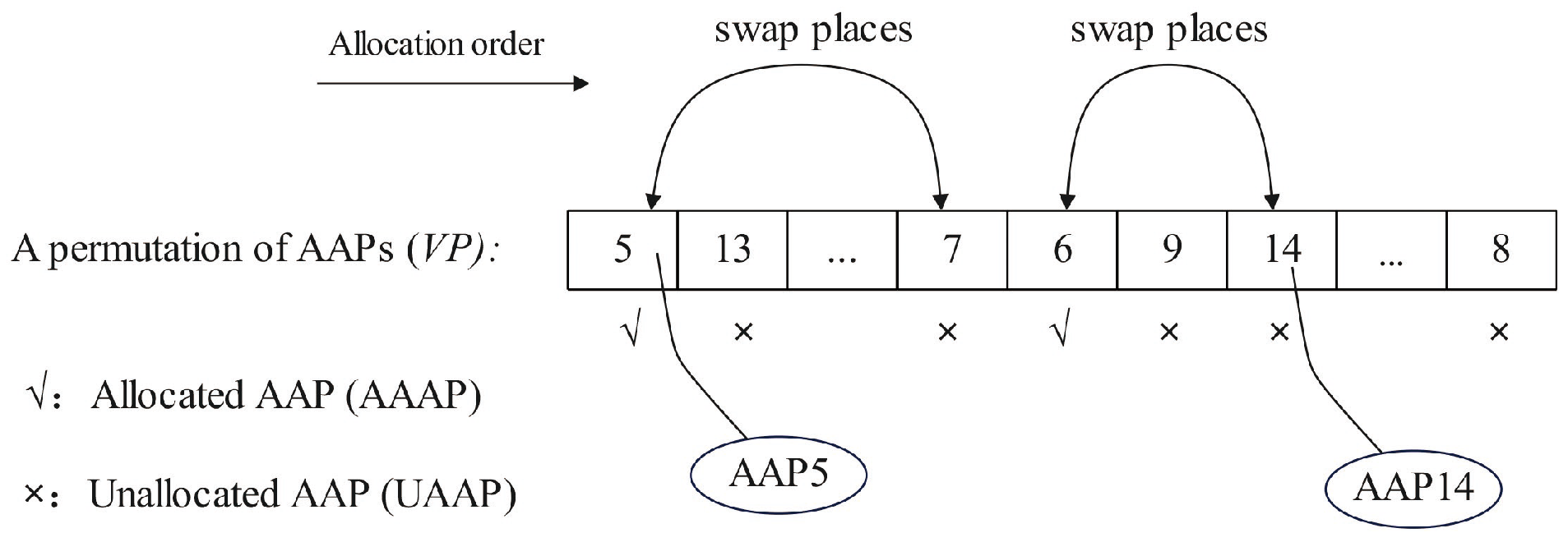
Through these two properties, we can know that exchanging the position of UAAPs that conflict against different AAAPs can generate new solutions; thus, an easy way to generate new solutions can be proposed. The specific operations called local search (LS) operation are as follows:

LS operation: Select m UAAPs from the $VP$, and for each UAAP, swap it with the nearest AAAP in front of it.

Note that $S_{UAAPs}$ is the set of all UAAPs in the $VP$. The parameter m is given by human. The set of new $VP$ that can be generated by LS operation is called the neighborhood of original $VP$. Obviously, the larger the value of m, the more individuals in the neighborhood of original $VP$. In order to save calculation costs, we set $m=1$ and then the corresponding neighborhood is relatively small. The illustration and pseudocode of LS operation are shown in Figure 2 and Algorithm 3.

Algorithm 3: Local search ($m=1$)

5.4. The Framework of MMRCH-LS

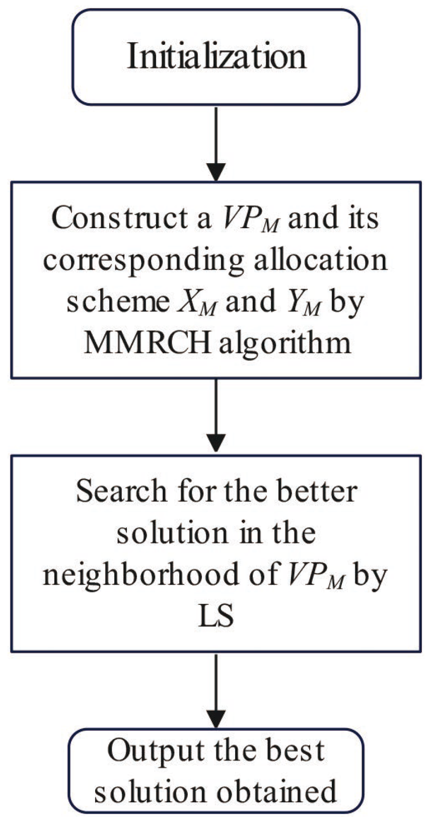
The maximum marginal return constructed heuristic algorithm with local search (MMRCH-LS) is shown in Figure 3, which combines the strengths of both MMRCH and LS operations.

Firstly, the related parameters are initialized, and then the MMRCH is used to construct a solution $V{P}_M$ with high objective value. To further improve the quality of the solution obtained, LS is used to find the best solution in the neighborhood of $V{P}_M$.

6. Performance Test

To prove the effectiveness of the designed MMRCH-LS algorithm in solving the USWTA problem, we set up a series of test instances and conducted simulation experiments, and then analyzed the simulation results.

6.1. Test-Instance Generator

Firstly, we develop a generator to generate initial parameters for the USWTA problem including ${\Phi }_{\xi ,k}$, ${\Phi }_{\gamma ,ik}$, ${\Phi }_{\eta ,ik}$, $q_{ik}$, $p_{jk}$, $m_k$, $n_k$ ($i=1,2,...,S;j=1,2,...,W;k=1,2,...,T$).

(1)

Generation of ${\Phi }_{\xi ,k},{\Phi }_{\gamma ,ik},{\Phi }_{\eta ,ik}$

The uncertain distribution of ${\xi }_k$, ${\gamma }_{ik}$, and ${\eta }_{jk}$ follow that ${\xi }_k\sim z(a_{\xi ,k},b_{\xi ,k},c_{\xi ,k})$, ${\gamma }_{ik}\sim L(a_{\gamma ,ik},b_{\gamma ,ik})$, and ${\eta }_{ik}\sim L(a_{\eta ,jk},b_{\eta ,jk})$, respectively. The detailed information is given in

Table 2. Parameter setting.

Parameter	Detail Information
$(a_{\xi ,k},b_{\xi ,k},c_{\xi ,k})$	Randomly valued in [1,10] within $a_{\xi ,k}<b_{\xi ,k}<c_{\xi ,k}$.
$(a_{\gamma ,ik},b_{\gamma ,ik})$	Randomly valued in (0,0.9) within $a_{\gamma ,ik}<b_{\gamma ,ik}$.
$(a_{\eta ,jk},b_{\eta ,jk})$	Randomly valued in (0,0.8) within $a_{\eta ,jk}<b_{\eta ,jk}$.

.

(2)

Generation of $q_{ik}$ and $p_{jk}$

The values of $q_{ik}$ and $p_{jk}$ are set as follows:

$$\begin{array}{c}{q}_{ik}=q_L+(q_H-q_L)·rand\\ p_{ik}=p_L+(p_H-p_L)·rand\end{array}$$

where $q_L$ and $q_H$ are the lower bound and upper bound of tracking probability of sensors, respectively. $p_L$ and $p_H$ are the lower bound and upper bound of the interception probability of weapons, respectively. They are all predefined constants within $0<q_L<q_H<1$ and $0<p_L<p_H<1$. Here, we set $q_L=0.72$, $q_H=0.96$, $p_L=0.5$, and $p_H=0.95$.

(3)

Generation of $m_k$, $n_k$

There are two cases to discuss here.

Case 1: Each target is allocated one sensor and one weapon at most, i.e., $m_k=1,n_k=1(\forall k\in \{1,2,\dots ,T\})$.

Case 2: The maximum number of sensors or weapons that can be allocated to a target are set to 1, 2, or 3 according the uncertain distribution of threat value of the target, i.e.,

$$\begin{array}{c}{m}_k=\left\{\begin{array}{c}1, if 0<b_{\xi ,k}\le 4\hfill \\ 2, if 4<b_{\xi ,k}\le 8\hfill \\ 3, if 8<b_{\xi ,k}\le 10\hfill \end{array}\right.\\ n_k=\left\{\begin{array}{c}1, if 0<b_{\xi ,k}\le 4\hfill \\ 2, if 4<b_{\xi ,k}\le 8\hfill \\ 3, if 8<b_{\xi ,k}\le 10.\hfill \end{array}\right.\end{array}$$

Note that Case 1 present the simplified USWTA problem and Case 2 present the original one.

6.2. Algorithms for Comparison

To prove the effectiveness of the designed MMRCH-LS, we adopt a random sampling (RS) algorithm as the main comparison algorithm.

The framework of RS is similar to that of MMRCH but the rule is abandoned. In each iteration of RS, we randomly generate a $VP$ and use CP to generate the corresponding allocation scheme. Apparently, RS is a random statistical method without the use of domain information accumulated during its sampling process. A series of feasible solutions are generated by repeating the above process within the running times permitted and select the best solution as the final output. Here, we set running times to 1000.

Meanwhile, in order to test the effect of LS in improving the quality of the solution, the MMRCH algorithm without LS is also adopted as a comparison algorithm.

6.3. Experiment Setup

In the simulation experiment, we preset 20 instances of USWTA problem, including 5 instances from Case1 and 15 instances from Case2. Give the basic parameters $S,W,T$ and other parameters are generated by the test-instance generator proposed in Section 6.1. The basic parameters of the 20 instances are shown in

Table 3. $S,W,T$ of 20 instances.

No.	$\mathit{SWT}$	No.	$\mathit{SWT}$
1 *	$S5W4T3$	11	$S21W18T20$
2 *	$S10W9T8$	12	$S28W20T23$
3 *	$S20W20T20$	13	$S30W35T28$
4 *	$S40W45T50$	14	$S45W50T38$
5 *	$S80W70T65$	15	$S62W50T30$
6	$S4W5T7$	16	$S70W72T56$
7	$S7W7T7$	17	$S80W85T67$
8	$S10W8T13$	18	$S90W100T110$
9	$S15W19T13$	19	$S150W140T130$
10	$S19W14T15$	20	$S180W170T175$

* means the instance belongs to Case 1, otherwise it belongs to Case 2.

.

Since RS is an algorithm with stochastic nature, it ran 20 times for each instance. The MMRCH-LS and MMRCH also ran 20 times in order to collect the data of runtime. A maximum acceptable time is set to 60 s. If the running time reaches or exceeds it, the output is deemed as invalid. The experiment was carried out in a MATLAB_R2018b environment on a PC with Intel Core i5 CPU 2.30 GHz and 12 GB internal memory.

6.4. Results and Analysis

The experimental results are shown in Figure 4 and

Table 4. The runtime (s) of MMRCH-LS, MMRCH and RS.

No.	MMRCH-LS	MMRCH	RS
1 *	0.0348 ± 8.42 × 10−4	0.0028 ± 6.62 × 10−4	0.0386 ± 2.00 × 10−3
2 *	0.0997 ± 5.15 × 10−4	0.0384 ± 4.57 × 10−4	0.1199 ± 0.0411
3 *	1.0754 ± 0.0382	0.5861 ± 8.2 × 10−4	0.7147 ± 0.0568
4 *	20.6079 ± 0.2017	18.1826 ± 0.1323	10.5079 ± 0.9322
5 *	n.a.	n.a.	n.a.
6	0.0549 ± 6.33 × 10−3	0.0167 ± 5.53 × 10−3	0.0537 ± 0.0163
7	0.0901 ± 0.0342	0.0256 ± 9.56 × 10−3	0.0761 ± 0.0287
8	0.2827 ± 0.0281	0.0658 ± 0.0105	0.1695 ± 0.0331
9	1.2783 ± 0.0433	0.3228 ± 0.0321	0.4141 ± 0.0353
10	1.3769 ± 0.0392	0.3178 ± 0.0285	0.4289 ± 0.0458
11	3.1187 ± 0.1047	0.7047 ± 0.1010	0.7191 ± 0.0412
12	4.5348 ± 0.1326	1.3645 ± 0.2041	1.1473 ± 0.0625
13	10.8739 ± 0.2286	4.5508 ± 0.3056	2.5840 ± 0.0589
14	28.6842 ± 0.5856	18.6987 ± 0.6128	9.7200 ± 0.1210
15	43.8781 ± 0.7134	24.0273 ± 1.0391	10.9021 ± 0.1580
16	n.a.	n.a.	15.4585 ± 0.4210
17	n.a.	n.a.	n.a.
18	n.a.	n.a.	n.a.
19	n.a.	n.a.	n.a.
20	n.a.	n.a.	n.a.

* means the instance belongs to Case 1, otherwise it belongs to Case 2.

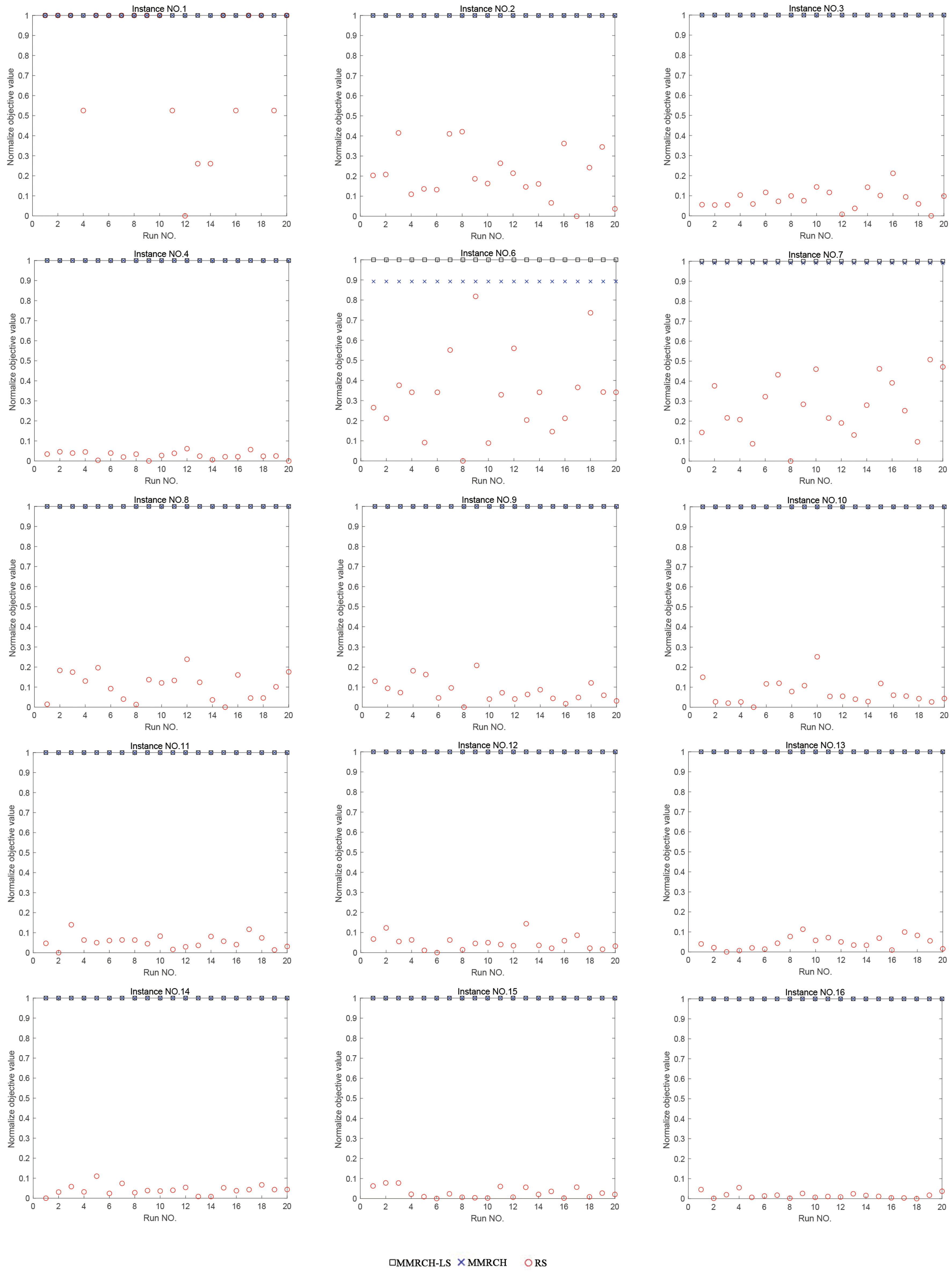
. Figure 4 shows the comparison of normalized objective function values obtained by the three algorithms for each instance. Notice that the objective function values are normalized from 0 to 1 by following formula:

$$\overline{f}=\frac{f-f_{\min }}{f_{\max }-f_{\min }}$$

where $f_{\min },f_{\max },f,\overline{f}$ are the minimum value, maximum value, original value, and normalized value obtained by the three algorithms, respectively. Table 4 shows the running time of three algorithms.

In Figure 4, the simulation results of instances including No.5, No.17 No.18, No.19, and No.20 are not displayed since the running time of the three algorithms in solving these instances exceeds the maximum acceptable time (60 s). From the comparison results of the normalized objective values in Figure 4, we can know that the MMRCH-LS and MMRCH can obtain the allocation schemes with high quality. Furthermore, with the scale of units (sensors, weapons, and targets) in the instance increasing, the quality of the allocation scheme obtained by MMRCH-LS and MMRCH algorithms is more and more superior to that obtained of the RS algorithm, which validates that the maximum marginal return rule in MMRCH can use the domain knowledge of problem to construct allocation scheme with high objective value effectively. Specifically, it can be seen from the comparison results of instances No.6 and No.7 that, after MMRCH constructs a high-quality allocation scheme, the LS operation can further improve the quality of it in the neighborhood. However, when solving the instances with large scale units, the LS operation has failed and can not found a better solution.

From the comparison result of running time of the three algorithms in Table 4, we can see that the real-time performance of MMRCH is unstable: When solving the instances with small scale units (No.1–No.3, No.6–No.11), the running time of MMRCH is less than that of RS. However, with the scale of units in the instance increasing, the running time of MMRCH and RS gradually increases, and the running time of MMRCH exceeds that of RS eventually (No.4, No.12–No.16). Additionally, it should be noted that the difference in running time between MMRCH-LS and MMRCH is caused by the presence or absence of LS operation, thus we can know that with the scale of units in the instance increasing, the running time of LS operation will also gradually increase, i.e., the real-time performance of LS operation decreases.

To calculate the computational time complexity of MMRCH and RS, we can start by calculating the time complexity of each lookup operation embedded in the iteration of algorithms. As for MMRCH, the complexity of a desirable lookup operation is $O\left(l\right)$, where l is the size of the AAPs for lookup and initialized to $S·W·T$. The size of l will decrease while a lookup operation ends: When the first AAP is added in the first loop, there are $A_1=1+(T-1)(W-1)+(T-1)(S-1)$ AAPs that are going to be deleted from ∂. For following $(S-1)$ times of the loop, the minimum number of AAPs to be deleted is $A_2=1+(W-1)(T-1)$ in each loop. Then, for the remaining AAPs, we can delete at least one AAP in each loop; thus, in the worst condition, l at $\beta$th loop can be calculated as follows:

$$l=\left\{\begin{array}{cc}\alpha \hfill & \beta =1,\hfill \\ \alpha -A_1\hfill & \beta =2,\hfill \\ \alpha -A_1-A_2(\beta -2)\hfill & \beta =3,\dots ,S+1\hfill \\ \alpha -A_1-A_2(\beta -2)-(\beta -S-1)\hfill & \beta =S+2,\dots .\hfill \end{array}\right.$$

As for RS, in each loop it only calculates the marginal return of one AAP, thus the desirable lookup operation of RS has the complexity of $O\left(1\right)$. Notice that the initialized $O\left(l\right)$ of MMRCH will increase rapidly with the scale of units in the USWTA problem increasing, and the integral calculation in Equation (15) (Line 17 in Algorithm 2) in each iteration will consume a lot of computing time, so the time consumption of MMRCH is higher than that of RS in solving the USWTA problem with large scale units.

Additionally, the allocation schemes and corresponding objective values of instances including No.1-No.3,No.6-No.10 obtained by MMRCH-LS are shown in

Table 5. The allocation schemes and objective values of some instances obtained by MMRCH-LS.

No.	Allocation Scheme of Sensors	Allocation Scheme of Weapons	Objective Value
1 *	(0 2 0 3 1)	(2 0 1 3)	4.4490
2 *	(4 3 1 8 2 7 0 0 6 5)	(1 4 7 5 0 3 8 6 2)	17.2214
3 *	(9 10 16 5 20 8 3 1 14 7 2 11 13 12 19 4 6 15 17 18)	(8 19 1 6 17 13 9 16 5 14 10 7 15 18 4 20 3 12 2 11)	54.9023
6	(6 6 7 3)	(6 6 3 7 6)	10.5315
7	(1 3 6 3 1 7 7)	(3 1 7 1 7 3 6)	15.6225
8	(6 11 4 9 12 7 7 8 4 11)	(7 7 8 11 9 4 12 6)	30.3581
9	(13 10 8 3 5 3 10 5 2 13 12 7 8 4 9)	(10 2 8 3 13 7 12 5 7 8 3 9 8 5 12 13 2 4 10)	44.0332
10	(3 5 12 6 1 13 2 5 7 3 6 7 12 2 4 12 3 15 1)	(6 1 7 3 13 3 7 2 12 15 4 5 13 6)	47.2940

* means the instance belongs to Case 1, otherwise it belongs to Case 2. The allocation scheme of sensors in instance No.1 means that the sensor 2 is allocated to target 2, sensor 3 is allocated to target 3, and sensor 4 is allocated to target 1; 0 means the unit is not allocated to any targets.

(The allocation schemes of other instances are too large to be displayed). From Remark 2 we can know that when a target is not assigned any sensors or weapons, assigning the weapons or sensors to it does not contribute to the objective value, but only wastes resources. Therefore, if a target is assigned a sensor or a weapon, then there must be a weapon or a sensor assigned to it as well. The results in Table 5 are consistent with it. To conclude, when solving the USWTA problem with small scale units, the MMRCH-LS designed in this paper can obtain the allocation scheme with high quality, and the real-time performance of it can also meet actual requirements. However, when solving the USWTA problem with large scale units, although the MMRCH-LS can also obtain the allocation scheme with high quality, its real-time performance is poor, and the LS mechanism is redundant.

7. Conclusions

The STA and WTA problems have been extensively investigated in previous studies, while its uncertainties are generally ignored. In this paper, an S-WTA problem was studied based on uncertainty theory, and an USWTA model was established. Based on the actual requirement in battlefield, a solution method based on the expected value principle was provided to convert the proposed unsolvable model to a deterministic one, which was a constrained binary programming problem with an NP-hard nature. To solve the model efficiently, a permutation-based representation and a corresponding construction procedure were introduced firstly to facilitate the generation of a feasible solution for the USWTA problem. On this basis, a constructive heuristic algorithm based on maximum marginal return rule (MMRCH) was designed, which could use the domain knowledge of the problem to construct a feasible allocation scheme with high objective value. Additionally, the LS operation was employed to further improve the quality of obtained solution. Finally, a set of instances was presented to be solved by designed algorithm named MMRCH-LS, and the performance of algorithm is analyzed. The result showed that the designed algorithm can obtain the allocation scheme with high quality for each instance and outperform other comparison algorithms, and the real-time performance of it can meet the actual requirements when the scale of units was not very large.

The work in this paper provided a mathematical analysis method and model support for solving the S-WTA problem in the indeterminate battlefield environment full of uncertainties and subjective reliability, and an efficient heuristic algorithm utilizing the domain knowledge of problem was designed to solve the proposed model. The results showed that the designed algorithm can obtain high-quality solutions when solving the USWTA problems with any scale units, and its real-time performance also meets the actual requirements when the scale of units is not very large. Meanwhile, the allocation schemes obtained also verified the feasibility of the proposed model.

Although MMRCH-LS could effectively solve the USWTA problem in most of the instances and obtained solution with high quality, but its real-time performance was not good when solving the instances with large units. This was mainly because the integral operation in iteration occupies a lot of computation time, and the shortcoming became obvious when the amount of AAPs was large. Furthermore, in only 2 of the 20 instances was the output improved by the LS operation, and thus the validity of this mechanism cannot be fully demonstrated. Therefore, in our future work, we will focus on the design of better heuristic rules and local search operators. We hypothesize that the performance of the algorithm can be enhanced in solving USWTA problem with large units if we designed it appropriately.

Additionally, this paper assumed that the damage degree of the target is the product of the degree of weapon interception and the degree of sensor detection, which neglected some complicated factors of the sensor–weapon system configuration in actual application environment. Therefore, in our future work, we will also focus on establishing a more reasonable model which can further reflect the actual situation of the S-WTA problem.