1. Introduction
A significant portion of piezo-devices operate in oscillation mode. Such devices include various medical equipment, energy harvesting and storage systems, and different types of actuators.
A comprehensive review of energy harvesting methods is presented in [
1,
2]. It includes multiple schemes of piezoelectric devices based on different types of ceramics. The well-known shapes for such devices are the cantilever beam, disk, cymbal transducer, and multi-layer stacked structures. In [
1], some examples of porous composites are presented, including a sea sponge-inspired composite with high porosity. For such a complex structure, the process of numerical modeling can be simplified by obtaining the effective properties of the material that allow ignoring the initial geometry of the body and using a regular or quasi-regular finite-element mesh in computations. This process can be based on the homogenization technique described in [
3], and it was demonstrated for a complex structure with metal inclusions in [
4]. In some cases, it may be useful to implement piezo-devices with composites of a specific structure. In [
5], a porous ceramic was used to build an effective energy harvesting device.
The effectiveness of such devices is evaluated when operating at a certain frequency, most often associated with resonance or anti-resonance. Finding the resonant frequencies of the device and the associated eigenmodes is an important step in modeling.
Finite-element software for such analyses is widely used in research and engineering. In the ACELAN-COMPOS package [
6], a set of tools for solving static problems with composites was created previously, including elastic, piezoelectric, and magneto-electric materials. In this paper, we extend the possibilities of the package by adding necessary modules for solving general eigenvalue problems.
In this research, the following mathematical model [
7] of an electroelastic body is considered:
The presented model corresponds to a boundary problem with multiple electroelastic mediums. We use the index
j to enumerate the bodies. The following notations are used in Equation (
1):
is the frequency of the vibrations,
is the stress tensor,
is the strain tensor,
is the displacement vector,
is the electric induction vector,
is the electric field vector,
is the mass force density vector, and
is the scalar function of the electric potential. The material properties are presented by
(density),
(the fourth-order tensor of the elastic stiffness moduli),
(the third-order tensor of the piezoelectric moduli), and
(the second-order tensor of dielectric permittivity). The damping coefficients are
,
, and
, while “
” denotes the double inner product operation for the tensors.
Mechanical boundary conditions are applied on the boundaries (
) as a displacement field on
such that
and as surface stress vector
:
Electrical boundary conditions are set on the surfaces with electrodes (
) and without electrodes (
,
):
To solve the above system numerically, we use the finite-element method. Equation (
1)’s continuous model is replaced by a vector model:
where
is the matrix of the form functions for displacement,
is the vector of the form functions for the electric potential, and
and
are the global vectors of the corresponding nodal unknowns. We will consider a problem without damping such that after the substitution
, the following system of linear equations is obtained:
where
is the global mass matrix,
is the global stiffness matrix, and
is the vector of the right-hand side obtained by discretization of the loads
. The structures of the matrices
and
are as follows:
where
M,
, and
are the symmetric positive definite matrices.
For the harmonic vibration at a natural frequency
, we have
where
v will represent the mode shape. Let us consider the free oscillation with
. The initial finite-element approximation may be rewritten as
The problem now has following form:
In this case, we have unknowns, where n is the number of elements in and the extra unknown is . The substitution leads us to the generalized eigenvalue problem (GEP) that will be discussed in this study.
Furthermore, we use lowercase symbols (not boldface) to denote vectors and lowercase Greek letters to denote scalars, while uppercase symbols are reserved for the matrices.
Let us consider the GEP
where
is a desired eigenvalue,
v is a corresponding eigenvector, and
is an eigenpair. The stiffness matrix
in Equations (
2) and (
3) is symmetric quasi-definite (SQD) (i.e., it is a non-singular indefinite matrix) [
8], and the mass matrix
is symmetric positive semi-definite (denoted as
).
The field of numerical methods for solving eigenvalue problems is in constant flux, with new methods and approaches continually being created, modified, tuned, and eventually, in some cases, discarded [
9]. The solution of the standard eigenvalue problem is still relevant. Therefore, in [
10], methods for solving a Hermitian eigenvalue problem based on the multi-step Rayleigh iteration (MRQI) as well as its inexact variant (IMRQI) were investigated for effective computations eigenpairs of a Hermitian matrix. In [
11], a general paradigm of nonstationary Richardson methods and gradient descent methods, called the parameterized power method, for computing the dominant eigenvalue and corresponding eigenvector of a real and symmetric matrix were constructed. This paradigm includes the power method as a special case [
11].
For huge matrices, the most promising approach is to use methods based on Krylov subspaces. To select the most effective approach, a comparative analysis of the methods and intended for solving both standard and generalized symmetric eigenvalue problems was carried out [
12]. The following methods have been investigated: the generalized power method [
11], the standard Lanczos method [
13], the Lanczos method with shift and inversion, and subspace iteration methods, as suggested in [
9,
14,
15]. A comparison of these methods showed that it is impossible to simultaneously satisfy mutually incompatible requirements, such as predetermined accuracy, reliability, speed of execution, reasonable memory requests, brevity of the program, and the possibility of efficient parallelization. In a particular computational problem, one or more of these requirements may not be present. When solving a standard eigenvalue problem [
12], the Lanczos method showed the best results in terms of efficiency and accuracy of calculations. The application of the “shift-and-invert” (SI) spectral transformation, which is necessary to search for internal points in the spectrum, was also tested. The extreme eigenvalues, when sufficiently separated from each other, were reliably found by the Lanczos algorithm.
The results obtained in [
12] showed that both partial and complete reorthogonalization of Lanczos vectors significantly improves the accuracy of calculations without requiring a lot of additional time (taking into account the parallelization of a number of operations, such as matrix-vector products). Therefore, when passing to the GEP, the choice was made in favor of Lanczos-type methods. These results are in good agreement with those presented in [
16]. This study states that some advantages can be obtained by applying this procedure explicitly when subspace iteration is used or implicitly by applying the Lanczos algorithm to the inverted operator. However, since the last method is a much more powerful one, it should be used whenever possible. The Lanczos algorithm is applied when the sought eigenvalues are well-separated and extremal [
16]. However, this research is limited to the case when both matrices in the GEP (Equation (
3)) are symmetric (Hermitian) and the mass matrix
is symmetric positive definite (SPD). In [
17], an attempt was made to apply the Lanczos method for solving Equation (
3), but because it converges very slowly, it is not used in practice. In [
18], conversely, a study of the GEP was carried out for the case of an SPD stiffness matrix and a semi-definite mass matrix.
An alternative approach to solving this problem is a stable generalization of the QR algorithm to arbitrary square pencils [
19]. This method is well known as the QZ algorithm. However, it breaks the symmetry and replaces the original pencil with an equivalent one that has two upper triangular matrices. Only orthogonal transformations are applied, and the final accuracy is not affected by such unpleasant circumstances as the singularity of the
. It takes about
operations to find all eigenvalues with the QZ algorithm, but the method cannot be applied to large-scale matrices.
A particularity of the problem considered in the study is the non-standard structure of the matrices included in the GEP. One of them is symmetric quasi-definite (i.e., indefinite), and the second matrix is singular. We did not find in the literature a solution to the GEP for such a class of matrices. Accordingly, large matrices that have to be inverted at each step of the SI Lanczos algorithm are indefinite, and standard methods for SPD matrices are not applicable for them. As a rule, many authors use the modified Cholesky decomposition to solve a system of linear algebraic equations (SLAE), but in our case, this was not applicable. The reason for this is that the matrix obtained as a result of the finite element approach described above is highly sparse (i.e, it has an overwhelming number of zero elements), but it does not have any ordered structure (e.g., banded, block, or profile). This generates practically filled triangular matrices in this decomposition.
Of course, Lanczos-type methods are not limited to the entire field of computational methods for solving both the standard and generalized eigenvalue problems. Of the most original approaches, we would like to mention [
20], whose author proposed solving the problem by combining the Jacobi–Davidson method with the conjugate gradients. The author considered the Jacobi–Davidson method with inner preconditioned conjugate gradient iterations for the arising linear systems and showed that the coefficient matrix of these systems is indeed positive definite, with the smallest eigenvalue bounded away from zero.
It should be noted that a particularly interesting and most complex GEP is the buckling eigenvalue problem, which can also be solved by the SI Lanczos method [
21]. In this problem, the matrix
is symmetric positive semi-definite, the matrix
is symmetric indefinite, and the matrix
is singular. Specifically,
and
share a non-trivial common nullspace, but this complex issue is beyond the scope of this article.
The purpose of this research is to evaluate the performance of the Lanczos method in solving the GEP for given classes of matrices (SQD stiffness matrix and singular mass matrix). This article is organized as follows. The peculiarities of the GEP with a singular mass matrix are described in
Section 2. “Shift-and-invert” spectral transformation for the GEP is considered in
Section 3. Numerical tests are given in
Section 4, and their results are discussed. The conclusions are presented in the last section.
2. Generalized Eigenvalue Problem
The pair of matrices
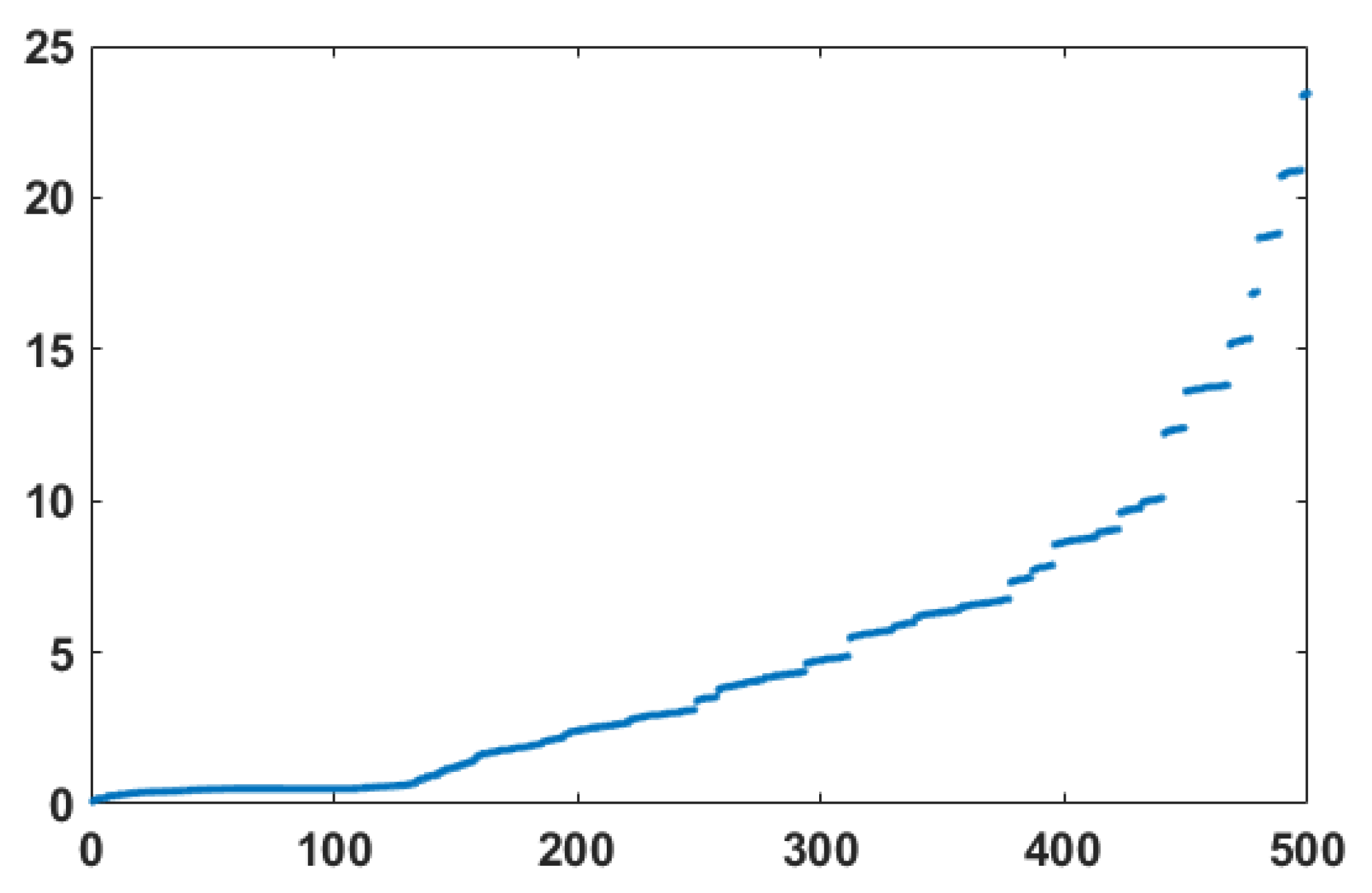
is called a matrix pencil. We will treat the case where a combination
is a positive definite matrix for some scalars
and
[
9]. This situation occurs despite the fact that neither
nor
are positive definite matrices in Equation (
3). An example for
and
is shown in
Figure 1 for the model matrices
(
). Here the first point of the spectrum has a value of 0.086275 and the last point is 23.443.
It then follows that all eigenvalues
of the GEP in Equation (
3) are real. Moreover, all eigenvalues are positive, and we have a symmetric definite pencil. This assumption is true for a wide class of practically important cases, and the theory is very closely related to the standard symmetric (or Hermitian) eigenproblems, except that some eigenvalues may be infinite [
9].
Therefore, we consider the simple Lanczos algorithm [
13,
14], although all reasoning applies directly to the block algorithms as well. Working with a large Krylov space is a very bad choice for large-scale problems because storing all the basis vectors requires too much memory. It should be noted that the Lanczos method cannot be used for solving the GEP immediately. In [
14], it is shown that this algorithm can be run directly on the pencil
, provided
is positive definite and that certain systems of equations with
can be solved. One way to improve the convergence rate is using a spectral transformation [
15].
We pay attention to issues that can occur when the mass matrix
is singular. Then,
has an incomplete rank, denoted as
r:
Additionally, the spectrum of the GEP (Equation (
3)) has only
r finite eigenvalues, where
, with the remaining
eigenvalues being at infinity such that
. In most practical cases, we are not interested in computing these infinite eigenvalues and interested in finite ones. The eigenvectors
associated with the eigenvalues at infinity belong to the null space of
; in other words, the following is true:
without any physical meaning. Note that the eigenvectors corresponding to the finite eigenvalues
can be
-orthonormalized such that
, where
is the Kronecker delta.
We can rewrite the problem in Equation (
3) as
where Equation (
6) has the same right eigenvectors
as Equation (
3) and its eigenvalues are reciprocals such that
. However, with such a formulation of the problem, the matrix
may lose symmetry and sparseness.
When the mass matrix
is singular, the Lanczos process proceeds with the semi-inner product defined by
. Such an inner product is mathematically correct within the Lanczos method [
22]. The use of the
semi-inner product restricts the computation of eigenvectors to those that are in the range of
. These are exactly the eigenvectors corresponding to the finite eigenvalues of the GEP in Equation (
3).
To measure the relative error between the exact solution and its approximation, we use the vector norm
In finite-precision arithmetic, the computed Lanczos and Ritz vectors have components in the nullspace of the matrix
, and the magnitude of these components grows during the iterations. Thus, for any vector
, where
and
, we have
(i.e., the semi-inner product does not see the components in the nullspace of
). These issues are overcome with the use of an appropriate starting vector, which must be put into the proper subspace [
23].
3. Shift-and-Invert Lanczos Algorithm for the GEP
When the matrices are very large, and the sparse direct eigensolvers are too expensive, a most natural approach in this case is to apply the SI Lanczos method to the
with or without shifts. Let us write the basic formulas for this. One has a real scalar
distinct from any eigenvalue, and we seek a few eigenvalues
close to
(perhaps together with their eigenvectors
v). The problem in Equation (
3) is changed into [
14,
15,
23]
where
is the identity matrix and
.
The spectral transformation is the Lanczos method applied to B. When lies close to the desired eigenvalue(s), the corresponding values are well-separated and extremal. Hence, they can be computed by the Lanczos algorithm. Operator B is not symmetric in the common case, but it is self-adjointed with respect to the inner product (i.e., ).
The Lanczos algorithm with a starting vector
b constructs a matrix
whose columns, called the Lanczos vectors, form the
-orthonormal basis for the
m-order Krylov subspace [
14,
15]
For
, the
-orthonormal Lanczos vectors are
,
, and the next vector
is obtained from the three-term recurrence
where
,
, and
when
such that
.
Let us write Equation (
10) in matrix form:
where
is the
mth column of the identity matrix
, the matrix
is such that
, and
is a symmetric tridiagonal matrix with
along the diagonal and
along the subdiagonal and superdiagonal. Since the columns of
are
-orthonormal to
, multiplying Equation (
11) by
gives
The
orthogonal projection of the eigenvalue problem
on the range of
gives the solution
with
and
. The residual is
and
is cheaply computed.
The shift-and-invert mode requires matrix-vector products of the form , where to be performed. In practice, the matrix is never formed explicitly, but an SLAE with the matrix is solved every time when the matrix needs to be multiplied by the vector. Usually, a direct method is used which allows to be factorized. Iterative methods can be applied for very large problems, but the SLAE needs to be solved more accurately than the desired accuracy of the eigensolution.
If we are interested in a few eigenvalues
near a specified shift
[
24], then the common strategy to determine the sequence of shifts can be employed in the SI Lanczos process for solving the GEP (Equation (
3)). For an arbitrary interval
, we denote with
and
the set of eigenvalues contained in the interval
and the set of eigenvalues from this interval calculated by the algorithm, respectively. In a given interval
, a sequence of shifts
is selected (and
for all cases). For each of the shifts
, the Lanczos method is applied to the matrix
. The choice of the shifts and the Lanczos process continue until
[
25].
The idea of using a sequence of shifts to calculate eigenvalues and vectors in turn is not new. However, the combination of shifts with the Lanczos process was proposed for the first time in [
25]. The efficiency of the algorithm strongly depends on how the shifts are chosen. The closer the eigenvalue
is to
, the better the separation of the corresponding
. Therefore, if one goes along
with a small step, then in each Lanczos run, only a small number of well-separated extreme eigenvalues needs to be calculated, and the convergence will be fast. However, in this case, it will often be necessary to factorize the matrix
, which is the most time-consuming operation of the process. Given an initial shift
, the sequence of shifts
chooses a new shift
,
such that the largest converged eigenvalue
is halfway between the old shift
and the new shift
(i.e.,
). In this way, if the eigenvalues are roughly evenly distributed across the spectrum, then the same number of eigenvalues is expected to converge to the left of the new shift as the number of eigenvalues that converged to the right of the old shift. The Lanczos iteration with a shift
is then stopped when all eigenvalues between the shifts
and
have been found [
23].
Thus, we used the algorithms described above to find the internal points of the GEP spectrum and the corresponding eigenvectors and further apply them to find the eigenvalues that lie in a given interval. To prevent the growth of the unwanted eigenvector components in the nullspace of the matrix
, we chose an appropriate starting vector which lies in the proper subspace of the
B (Equation (
9)). Next, we employed all these methods to find the natural frequencies of the electroelastic materials in numerical modeling.
4. Numerical Experiments
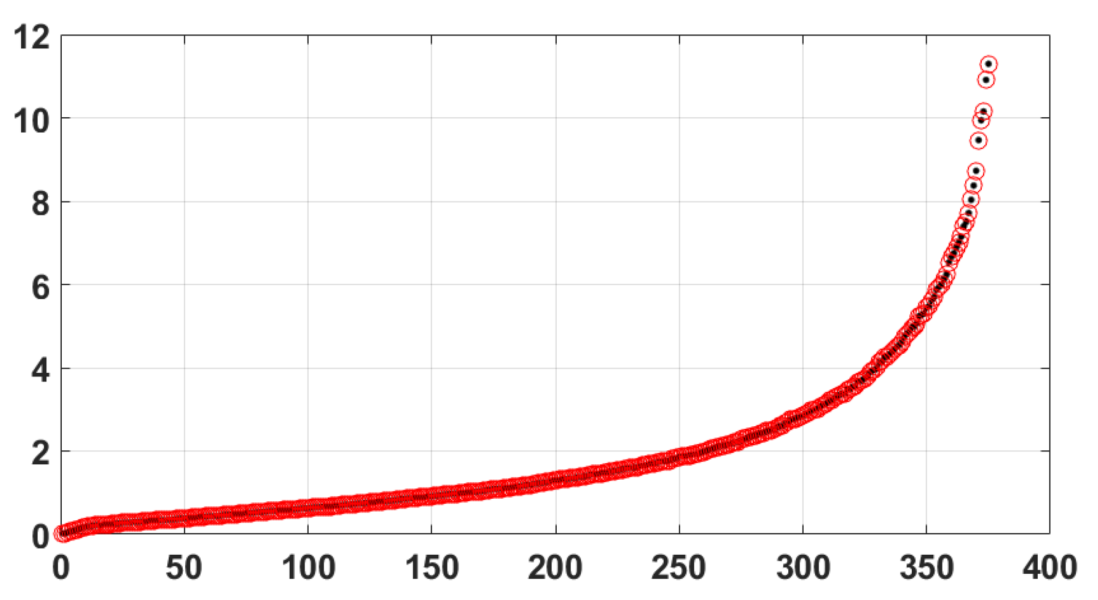
Unfortunately, we do not know the exact solution of the problem in Equation (
3). Therefore, to make sure the calculations were the correct numerical results, we first compared them with the MATLAB solution for the model GEP with matrices
,
. For the non-zero matrix block
in (
2),
, we used the Krylov subspace dimension
to check the coincidence of eigenvalues across the spectrum. In
Figure 2, we show the MATLAB-solution of the problem (black dots) and Ritz values obtained by the SI Lanczos algorithm (red circles). This pencil had 375 positive real finite eigenvalues, and the remaining
ones were
, corresponding to the infinity eigenvalues of the matrix
B, which were equal to zero.
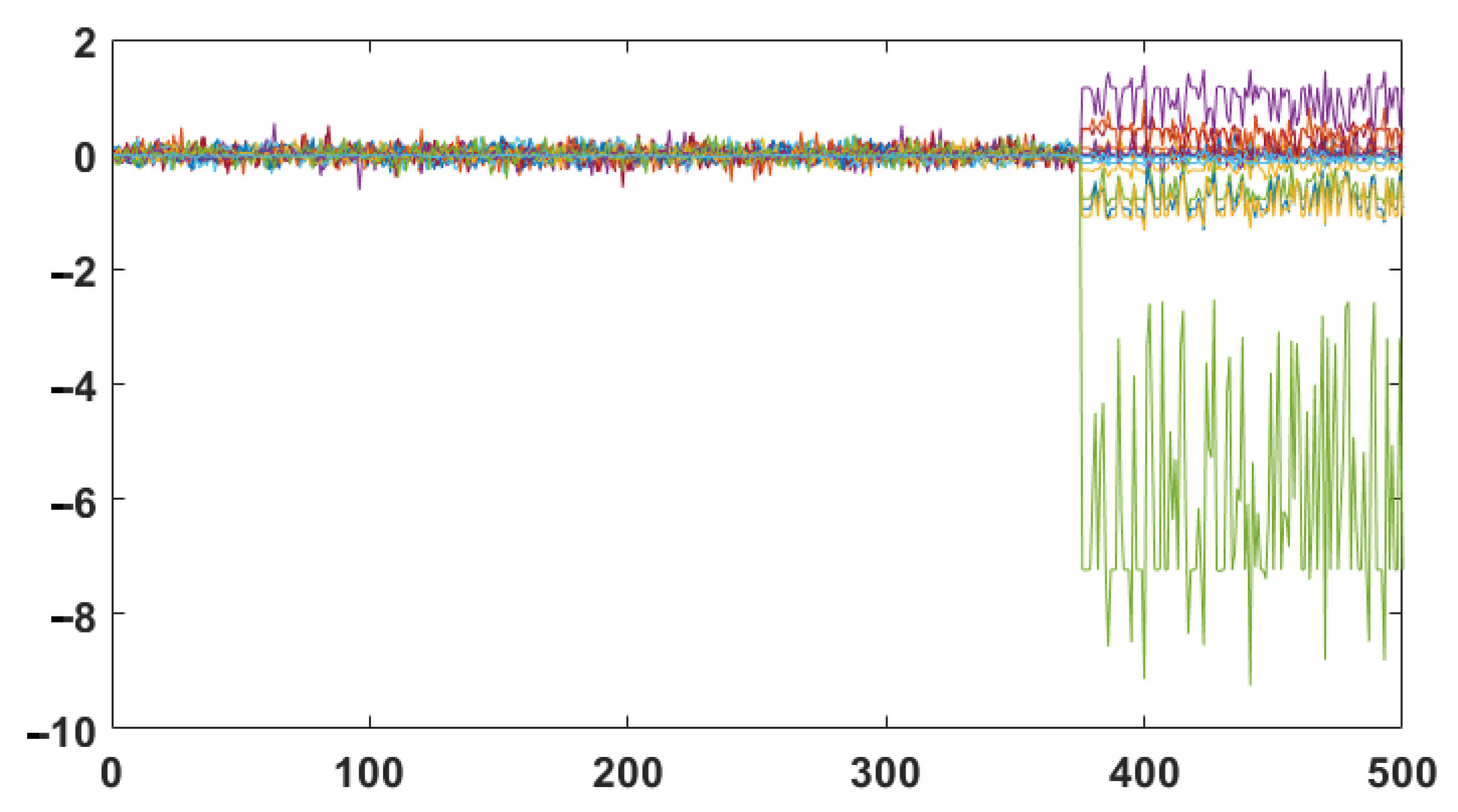
Figure 3 demonstrates the strong growth of the Ritz vector components, which were in the nullspace of the matrix
. The usual way to correct these unwanted components is to apply
B (Equation (
9)) to a random starting vector in
(we used the unit vector). Then, it would be confined to a range
.
The Ritz vectors obtained after this correction are shown in
Figure 4. Moreover, full reorthogonalization was carried out to guarantee the orthogonality of the Lanczos vectors. Without reorthogonalization, they quickly lost orthogonality, which led to the algorithm returning copies of the already-converged eigenvalues [
14].
factorization of the symmetric quasi-definite matrix was used for solving the SLAE. In [
4], it was shown that SQD matrices are strongly factorizable (i.e., for every permutation
P, there exist a diagonal
D and a unit lower-triangular
L such that a Cholesky factorization exists). The eigenvalues of the tridiagonal matrix
were found using the QR algorithm.
In what follows, we will call the MATLAB solution “exact” (denoted with
) and compare it with the Ritz values (denoted with
). In
Figure 5, we show the 9 eigenvalues closest to 6 (
, Krylov subspace dimension
).
The numerical results are given in
Table 1. As expected, the eigenvalues closest to the given value
converged with the best accuracy. Specifically, for seven of them (
), the estimate was correct [
24]:
where
is the bottom element of the normalized eigenvector of
, corresponding to the Ritz values
,
from Equation (
11).
In
Figure 6, we show all converging eigenvalues in the interval
and found as in [
23]. The convergence of the eigenvalues was estimated from the
norm of the residual.
It is interesting to compare the obtained results with the solution to the problem using SLAE iterative solvers. As suitable iterative methods, we used SYMMLQ or MINRES [
26], which were specially developed to solve indefinite SLAEs. These methods are able to solve equation systems with a required accuracy at each iteration step. The results of the search for the desired eigenvalues practically did not differ from those presented in
Table 1 when a direct solver was used. Therefore, for large matrices, it is quite possible to apply these iterative methods at each step of the SI Lanczos algorithm. Numerical experiments for the model problem were carried out in MATLAB (R2019a).
The presented method was also implemented in the ACELAN-COMPOS [
6] package. This consists of multiple computational modules based on a class library that implements the finite-element method. This library was implemented using the C# programming language and .NET platform. The package uses sparse matrix representation for global stiffness and mass matrices.
The modules for creating a mesh generation for various composites, solvers for systems of linear equations in single-thread mode, boundary condition handling, material importing, and post-processing were already implemented in the package [
27]. Specifically, for this study, new modules were added, including mass matrix assembling, which was not required for static problems, and methods and data structures related to the Lanczos method, namely the Krylov subspace and operations for it, such as reorthogonalization. The solver for the system of linear equations was updated to handle large matrices by adding the possibility to run matrix-vector multiplication in parallel mode for the selected sparse matrix storage formats.
We will examine two eigenvalue problems with simple geometries, presented in
Figure 7.
The initial step of the analyses was to obtain the elemental local matrices of mass and stiffness for each element. Hexagonal elements were used for meshing simple geometries in the ACELAN-COMPOS package due to its main purpose of working with representative volumes of composites. This allowed us to use regular meshes in some cases and store elemental matrices in a cache to reuse values for elements of the same size and material. It was also easy to control the nodal enumeration to obtain more convenient sparse matrix representation. Each local matrix was obtained by performing several steps. First, we computed the Jacobian matrix to transform the global coordinates of the finite element to become local. After that, we built the strain-displacement matrix for elastic materials or its analogue for electrostatic and piezoelectric materials. Let us denote this matrix as
. The next step was numerical integration over the element for the following expression:
Here, matrix
represents a corresponding matrix of the material properties. At each integration point, we evaluated the expression
and computed the weighted sum of values to complete numerical integration. In this research, we used linear elements with eight nodes and eight integration points. The computed local matrices had to be placed in a global matrix while considering the global enumeration of nodes and degrees of freedom for each node [
28].
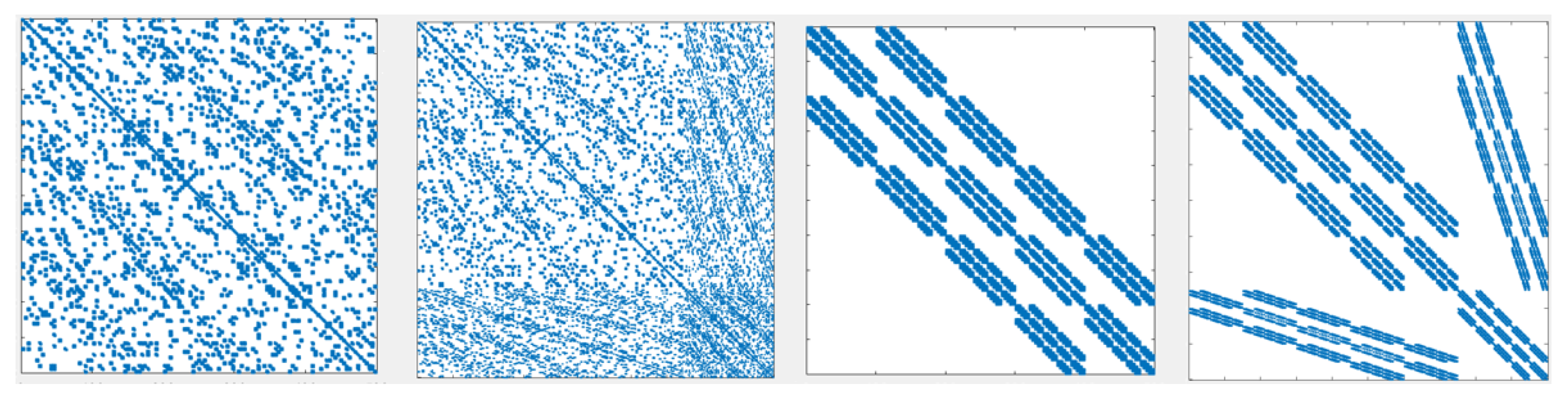
Multiple formats of sparse matrix storage used in the package involved the initial assembling of global matrices performed in triplet form. The matrix was stored as a hash table of pairs (position, value) that allowed adding new elements fast. However, the triplet format is not suitable for matrix-vector computation, which is the most significant operation in iterative computational methods used in this study. Therefore, we used the Compressed Sparse Row (CSR) or Compressed Sparse Column (CSC) format. As we mentioned, the positioning of non-zero elements in matrices depends on enumeration. The electrostatic problem with 125 nodes has 500 unknowns, since there are 3 components of displacement and 1 value for the electric potential. Four different types of enumerating for the same stiffness matrix with 500 rows are shown in
Figure 8.
It can be seen that the last of the enumeration corresponded to the matrix structure in Equation (
2). This version of the matrix can be built by ordering the node numbers by the X, Y, and Z axis consequentially and numbering the unknowns as
where
u represents the mechanical unknowns and
represents the electric unknowns. This structure of the matrix can be obtained for models with the same topology presented in
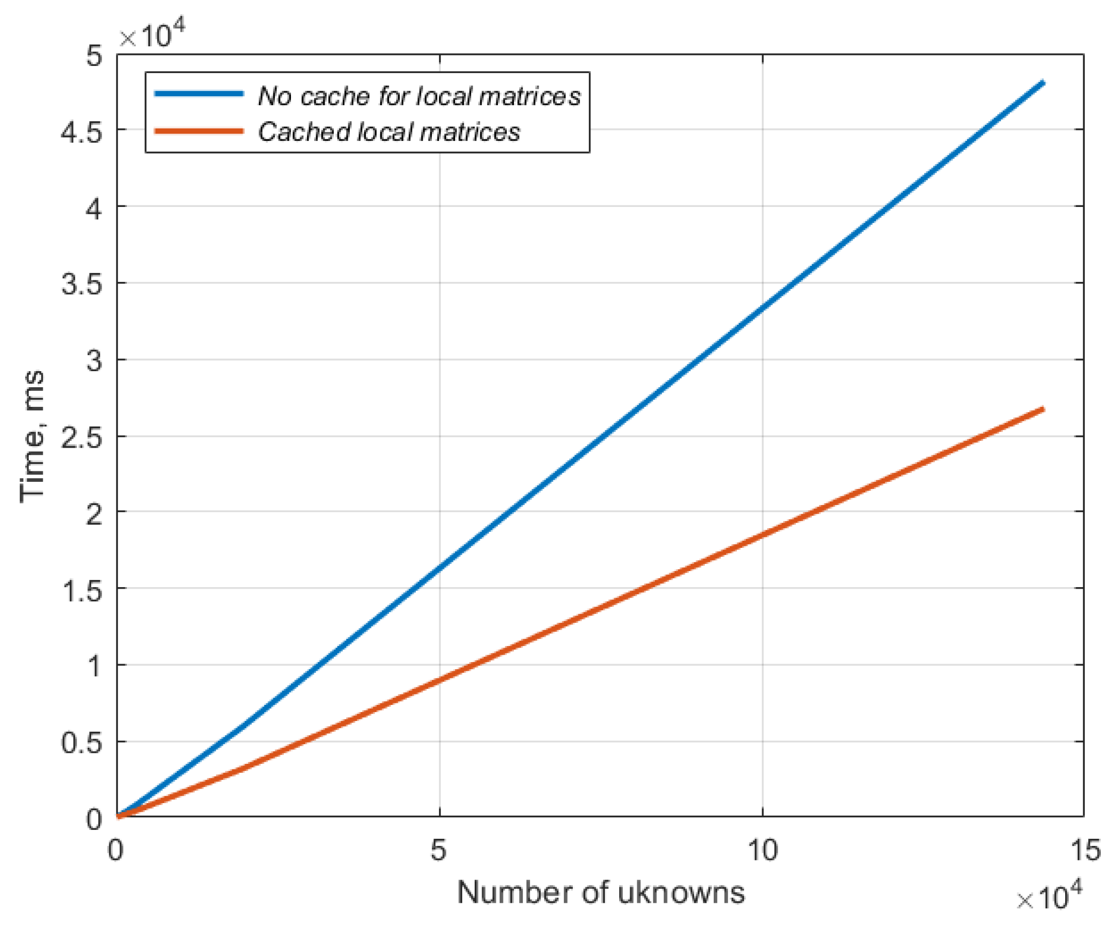
Figure 8. Assembling the global matrices usually requires computations of each local matrix. However, in some cases, we can use a uniform mesh that allows caching the local matrices for each material present in the model and reuse it in the step of building the global mass and stiffness matrices. The difference in time of assembling data for models with different numbers of unknowns is shown in
Figure 9. This was computed for a series of problems with 108, 500, 2916, 19,652, and 143,748 unknowns and interpolated for other values.
The assembling process happened in the triplet format and resulted in two data structures: actual and symbolical matrices. The latter was used for handling the boundary conditions. When we needed to apply fixed, constrained conditions, operations on specific rows and columns should have been performed. A symbolic matrix allows reducing the number of read and write operations by accessing the non-zero elements only.
For computational purposes, we transformed the matrix to the CSC storage format. The transformation time had a linear dependency on the size of the matrix. In the numerical examples, the matrix of the problem with 143,748 unknowns was transformed in 0.4 s, so this step had no significant outcome on the performance. Another widely used format, Skyline Storage (SKS), was also tested, but the width of the band was too big even after re-enumeration of the unknowns. While transformation from triplets had almost the same duration as for CSC, the numerical operations took significantly more time.
For implementation of the SI Lanczos algorithm, we used
factorization provided by the CSPARSE library [
29]. Since the inverted matrix obtained significantly more non-zero elements compared with the initial one, the reasonable numerical solving number of unknowns in the problem was quite limited.
factorization was replaced with an iterative process for solving SLAEs in some numerical experiments. For that purpose, we used a custom implementation of the SYMMLQ method [
26] for the CSR sparse matrix format. Since the main operation in this method is a matrix-vector multiplication, we used a simple parallel technique based on splitting the rows of the matrix into equal groups. Possible improvements to this approach based on the block structure of the stiffness and mass matrices are topics for future research.
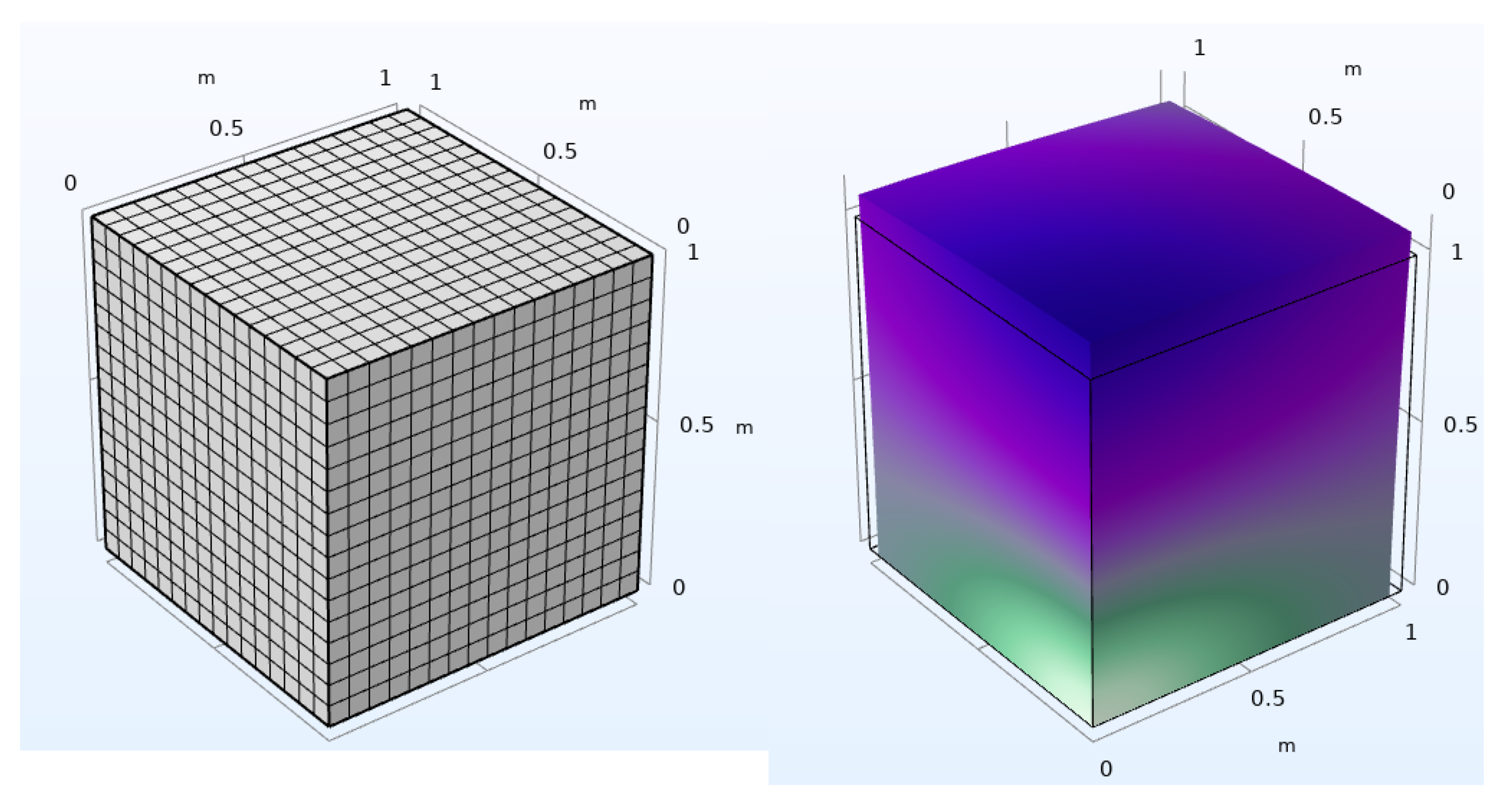
The developed method was tested in comparison with the COMSOL Multiphysics® package [
30] to compute the eigenvalues of a demo model with a regular mesh, as shown in
Figure 10.
The first eigenfrequency was 671.52 Hz in COMSOL and 709 Hz in ACELAN-COMPOS. For simplicity of comparison, the model was designed as an electrostatic cube. The boundary conditions were set to
,
,
,
, and
. This problem had a matrix with 19652 rows in ACELAN-COMPOS. In the COMSOL package, nonlinear elements were used, so the number of unknowns was 92,292. More accurate elements used in COMSOL may be the reason for the difference in the output values. In terms of performance, the ARPACK [
31] package used in COMSOL outperformed the current implementation of the SI Lanczos algorithm in the ACELAN-COMPOS package by huge margin. Performance analyses of the computational time for the problem with 19,652 unknowns showed that the CSR storage format was very convenient in terms of its small memory footprint. Up to 95% of the computational time was spent on solving the SLAEs with the SYMMLQ method. We used a fixed limit of 300 iterations for each solution. Further performance improvements may be obtained by fully utilizing the structure of the sparse matrices presented in the computations, including the symmetry, structure of the blocks, and possibility to perform more efficient parallel matrix-vector multiplication.
A simple parallelization technique was implemented for the SYMMLQ method with a CSR-stored matrix. Since the data structure allowed easily accessing all non-zero elements of a selected row without allocating extra space, the method for performing dot multiplication for sparse and dense vectors was written. The whole matrix-vector multiplication used in the method was divided into such operations, each contributing to a single element of the resulting vector. For the performance analyses, the same hardware was used for both the single-thread and parallel versions of the solver. Using 8 threads to perform the shift-and-invert Lanczos method with parallelized SYMMLQ resulted in a 40–45% speed up for the problem with 19652 rows.


