A Novel Multi-Agent Model-Free Adaptive Control Algorithm for a Class of Multivehicle Systems with Constraints

Abstract

To solve the problem of longitudinal cooperative formation driving control of multiple vehicles, a model-free adaptive control algorithm with constraints (cMFAC) is proposed in this paper. In the cMFAC algorithm, a dynamic linearization technique with a time-varying parameter pseudo-gradient (PG) is used to linearize the multivehicle collaborative system. Then, a cMFAC controller is designed. The algorithm sets the input and output constraints at the same time to prevent the vehicle speed and other parameters from exceeding the specified range. The main advantage of the cMFAC algorithm is that the entire control process only needs the input and output data of each vehicle and can effectively handle the input and output constraints. In addition, the stability of the cMFAC method is verified through strict mathematical analysis, and its effectiveness is verified with semi-physical experiments based on a MATLAB/Simulink module and CarSim platform connection environment. It is worth noting that the proposed cMFAC controller is symmetric because the input cost function and PG cost function have symmetric and similar structures, and the forms of the two cost functions are the same.

1. Introduction

Longitudinal multivehicle collaborative queue control is one of the important directions in the field of intelligent networked vehicles [1]. When the vehicles on a road achieve orderly formation driving, the energy consumption of each vehicle can be reduced by reducing the air resistance [2,3]. Longitudinal multivehicle collaborative queue control refers to control using wireless communication technology between vehicles. Using individual own on-board sensors, the driving status information of other vehicles in the queue can be obtained, corresponding driving decisions can be made, and an ideal distance between vehicles can be maintained to ensure queue driving stability [4,5].

Many scholars have carried out research on the longitudinal collaborative control of multivehicle queues. Reference [6] proposed a model predictive control (MPC)-based scheme to optimize the longitudinal multivehicle collaborative queue control system. Reference [7] proposed a linear quadratic control framework, established a nonlinear low-order vehicle dynamics model, and applied it to the longitudinal collaborative control of a multivehicle queue. In [8], the stability boundary was combined with a multiobjective clustering (MOF) algorithm to design a controller to achieve a stable and rapid high-speed vehicle queue. Reference [9] established a switched queue control model reflecting the influence of the following vehicle connectivity state on the queue controller through the designed vehicle spacing strategy. Based on this, an effective queue control algorithm was proposed. In reference [10], a new integral synovial control strategy scheme was adopted to achieve the longitudinal coordinated control of a multivehicle queue with uncertain disturbance.

In the process of controller design, the above methods are based on accurate mathematical models. However, almost all vehicle formations are difficult to build accurate system models. Clearly, it is not appropriate to establish an accurate dynamic model for a longitudinal multivehicle collaborative queue system to design the control system. To solve the inaccurate modeling problem of vehicle collaboration, data-driven control (DDC) has become the first choice.

A series of DDC methods, e.g., synchronous perturbation random approximation [11], unfalsified control [12], the virtual reference feedback tuning (VRFT) algorithm [13], iterative feedback tuning (IFT) [14], the iterative learning control (ILC) algorithm [15], and the model-free adaptive control (MFAC) algorithm [16] have been developed. Among the above DDC techniques, the MFAC algorithm has the advantages of small computation and strong adaptability. It has an ideal control effect and strong robustness for nonlinear systems. MFAC has achieved extensive applications in many fields, such as communication network computation [17], AC/DC microgrids [18], freeway ramp metering systems [19], and network systems [20].

In an actual longitudinal multivehicle cooperative queue system, there will be some constraints on the vehicle input and output (I/O) data (such as the upper limit of vehicle speed and acceleration) [21,22], which will affect vehicle control. Therefore, it is of great practical significance to consider an MFAC method that can handle the constraints.

To solve the multivehicle cooperative control constraints and realize the longitudinal cooperative control of a multivehicle fleet, a constraint model-free adaptive control algorithm (cMFAC) based on partial form dynamic linearization (PFDL) is proposed. In the cMFAC algorithm, based on consistency control, the upper and lower limit constraints are imposed on the input and output, and the cMFAC formation strategy is obtained.

The contributions of this work are as follows: A novel cMFAC method is proposed to solve the longitudinal multivehicle cooperative queue control problem synchronically with I/O constraints. The cMFAC scheme is a DDC approach that only requires the I/O data of the controlled objects, which means that the specific vehicle model is no longer needed. Therefore, it is very portable and can be used in different vehicles. The cMFAC can effectively ameliorate the impact of I/O constraints and ensure that the vehicles in the fleet track the desired trajectory.

The outline of this manuscript is as follows: In Section 2, the longitudinal vehicle driving dynamic analysis process is studied. Section 3 introduces the cMFAC algorithm. Section 4 introduces the simulation results of the cMFAC algorithm. Section 5 summarizes the main conclusions of this manuscript.

2. Vehicle Dynamics and Kinematic Process Analysis

In multivehicle fleet longitudinal collaborative control, as shown in Figure 1, all vehicles can rely on the technical advantages of workshop communication to obtain the motion state and changing trend of the front vehicle and the leader vehicle, simultaneously transmit their own motion state information (speed and acceleration) to other vehicles in real time, and control the vehicle spacing of each vehicle to improve driving stability.

The stability of a single vehicle is the basis of the formation system stability. It is necessary to analyze the longitudinal dynamic model of a single vehicle when analyzing the longitudinal queue system. The overall stress analysis is shown in Figure 2.

First, some vehicle assumptions are made to simplify the vehicle model:

(1)

In the process of driving, there is no coupling between the transverse and longitudinal motion;

(2)

The mass of the vehicle is fixed during driving;

(3)

The sideslip of the tires is ignored.

The output torque of the engine is defined as T (N · m). When the output torque is obtained, the vehicle converts the output torque to the driving torque through the transmission system. The driving torque $T_q$ can be obtained using the following formula:

$$T_q=T{i}_0{i}_g\eta ,$$

(1)

where $i_0$ is the transmission ratio of the rear axle final drive, $i_g$ is the transmission ratio, and $\eta$ is the transmission efficiency. The relationship between the driving force $F_t$ and the driving torque $T_q$ can be obtained through the following equation:

$$F_t=T_q/r,$$

(2)

where r is the rolling radius of the vehicle tires. Combining Equations (1) and (2), $F_t$ can be expressed as

$$F_t=T{i}_0{i}_g\eta /r.$$

(3)

Next, the resistance f is further analyzed and roughly divided into three categories. The air resistance $F_{air}$ suffered by the vehicle during driving is the first. It can be expressed as the following formula:

$$F_{air}=C_d{A}_{y}p{v}^2/2,$$

(4)

where $C_d$ represents the air resistance coefficient, $A_y$ represents the windward area of the vehicle (m², $\rho$ represents the atmospheric density at 25 °C, and $v=v_w+v_x$, where $v_w$ represents the wind speed, and $v_x$ represents the longitudinal speed of the vehicle.

The second type of resistance is the friction between the vehicle and the ground and the energy generated by the deformation of the vehicle tire and the ground when it leaves the current contact surface, namely, the rolling resistance. Therefore, the second type of resistance can be expressed as the following formula:

$$F_{\mu }=f_{g}mg\cos \vartheta ,$$

(5)

where $f_g$ is the rolling resistance coefficient, and $\vartheta$ is the gradient of the road.

The third type of resistance refers to the resistance caused by the gradient of the vehicle due to the existence of an incline, that is, the resistance caused by the component force of the vehicle’s own gravity when driving on an incline, namely,

$$F_{gravity}=mg\sin \vartheta ,$$

(6)

where m is the vehicle mass (kg), and g is the gravitational acceleration (m/s²).

To complete the vehicle longitudinal dynamic analysis, the longitudinal dynamic process can be described by the following equation:

$$ma\left(k\right)=F_t-f=F_t-F_{air}-F_{gravity}-F_{\mu },$$

(7)

where $a\left(k\right)$ represents the acceleration of the vehicle at time k. Equations (3)–(6) can be combined and substituted into Equation (7) to obtain

$$ma\left(k\right)=\frac{T{i}_0{i}_g\eta }{r}-\frac{1}{2}{C}_d{A}_{y}p{v}^2-mg\sin \vartheta -f_{g}mg\cos \vartheta .$$

(8)

The vehicle longitudinal dynamic analysis is thus completed.

In longitudinal multivehicle cooperative driving, the input is the real-time acceleration of each vehicle, that is, the torque of the vehicle, and the output is the distance between vehicles. Since the vehicle acceleration is not constant, and there are many uncontrollable factors in the actual control process, the relationship among them is actually nonlinear. To facilitate the description, considering other external factors, the distance and vehicle output torque can be converted into a typical nonlinear single input–single output (SISO) system, as shown below.

$$d_i(k+1)=W_i(d_i\left(k\right),\dots d_i(k-n_d),T_i\left(k),\dots T_i(k-n_T)\right),$$

(9)

where $\mathit{W}{(\dots ):R}^{{\mathrm{n}}_d+{\mathrm{n}}_T+2}\mapsto R$ is an unknown nonlinear function; $d_i\left(k\right)\in R$ is the control output, that is, the distance between the ith vehicle at time k and the leader vehicle; and $T_i\in R$ is the control input, that is, the engine output torque $T(N·m)$. $n_d\in z^{+}$ and $n_T\in z^{+}$ are unknown. System (9) is the general model of most existing multiagent systems.

3. cMFAC Controller Design

A multivehicle cooperative formation system is essentially a typical multiagent system (MAS). To solve the problem of longitudinal multivehicle cooperative control, in this section, a cMFAC algorithm is proposed based on a PFDL data model. In Section 3.1, some preliminary knowledge is introduced. In Section 3.2, the longitudinal vehicle queue dynamic system is dynamically linearized. In Section 3.3, the controller is designed, and the stability of the cMFAC algorithm is considered.

3.1. Background Information

(1)

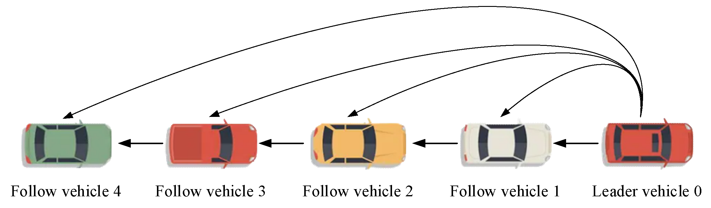
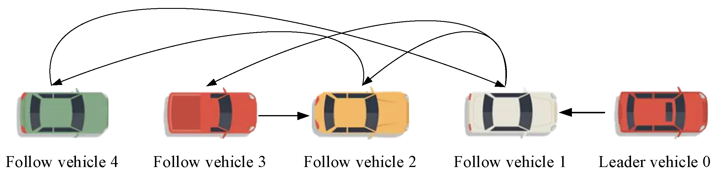
Graph theory

In MAS research, graph theory is an important analysis tool that can simulate the information exchange between agents. Here, we briefly introduce some basic concepts related to graphs and some basic properties of related matrices.

Consider that there are N agents in a network, and use node i to represent the ith agent, where $i\in \left\{1,2,\dots ,N\right\}$. If agent j can receive information from agent i at the current time, it is said that the edge from node i to node j is connected; otherwise, it is said that there is no connected edge between node i and node j. The connection topology is formed when agents exchange information with each other.

The symbol $\mathcal{G}=(\mathcal{V},\mathcal{E},\mathcal{A})$ in graph theory represents a topology, where $\mathcal{V}=\left\{1,2,\dots N\right\}$ represents a set of N system nodes, $\epsilon \subseteq v\times v$ denotes an edge set $\mathcal{G}$, and $\mathcal{A}=\left[a_{ij}\right]$ is the weighted adjacency matrix. If agent i can receive information from agent j, $a_{ij}=1$; otherwise, $a_{ij}=0$. $N_i=\{j\in \mathcal{V}|(j,i)\in \mathcal{E}\}$ represents the neighbor set of agent i.

The Laplacian matrix $L=\mathcal{D}-\mathcal{A}$ of graphs is an important research object in algebraic graph theory. It is not only an important tool for characterizing graphs but also the basis for proving whether a MAS converges. Suppose $\mathcal{G}$ is an undirected graph, and the indegree $\mathcal{D}$ matrix is defined as $\mathcal{D}=diag({\lambda }_1,{\lambda }_2,\dots ,{\lambda }_N)$ with diagonal entries ${\lambda }_i={\sum }_{j=1}^N{a}_{ij}$.

If there is a vertex that has no parent node but has a directed path to any other node, then $\mathcal{G}$ has a spanning tree. Additionally, a directed graph is said to be strongly connected if there is a directed path from any vertex of the graph to a different vertex.

Assumption A1. 

There must be one or more follower agents who can receive a message from the leader, and the topology $\mathcal{G}$ is a fixed strong connection.

Lemma 1 

([23]). Let $Q\left(k\right)\in R^{N\times N}$ be an irreducible subrandom matrix, and let Q represent the set of all possible $Q\left(k\right)$. There is a constant $\omega ,(0<\omega <1)$ that makes the product of n matrices satisfy:

$$∥Q\left(1\right)Q\left(2\right)\dots .Q\left(J\right)∥\le \omega ,$$

(10)

where $∥X∥$ is the Euclidean norm, and $Q\left(1\right),Q\left(2\right),\dots .Q\left(k\right),k=1,2\dots J$ are J matrices arbitrarily selected from Q.

(2)

Notation

The specific meanings of some symbols in this manuscript are explained as follows: R represents a real number, $R^n$ represents n-dimensional real vectors, and $R^{n\times m}$ represents $n\times m$ real matrices. I denotes the identity matrix, and $diag\left(\mathcal{A}\right)$ denotes the diagonal matrix. $a_{ij}$ in matrix $\mathcal{A}=\left[a_{ij}\right]\in R^{n\times m}$ represents the elements of row i and column j.

3.2. Dynamic Linearization

Regarding system (9), the following assumptions are made:

Assumption A2. 

The partial derivative of the output $y_i\left(k\right)$ in Equation (9) is continuous.

Assumption A3. 

System (9) satisfies the general Lipschitz, which means, for any $k>0$,

$$\mathsf{\Delta }{d}_i(k+1)\le \mathsf{{\rm Y}}∥\mathsf{\Delta }\mathit{T}i\left(k\right)∥,$$

(11)

where $\mathsf{{\rm Y}}>0$ is the Lipschitz constant, $\mathsf{\Delta }{T}_i\left(k\right)={\left[\mathsf{\Delta }{T}_i\left(k\right),\dots ,\mathsf{\Delta }{T}_i(k-\mathcal{Z}+1)\right]}^T$, and $\mathcal{Z}\in Z^{+}$ is the control input linearization length constant (LLC). $\mathsf{\Delta }{T}_i(k+1)=T_i(k+1)-T_i\left(k\right)$, $\mathsf{\Delta }{d}_i(k+1)=d_i(k+1)-d_i\left(k\right)$.

Remark 1. 

From a practical application perspective, Assumptions 2 and 3 are sensible. Assumption 2 is a typical term for a system that is generalized nonlinearly. Assumption 3 restricts the system output change rate. During actual movement, the speed of the manipulator cannot be unlimited, and the braking torque cannot be infinite.

Theorem 1. 

When system (9) satisfies Assumptions 2 and 3 with $∥\mathsf{\Delta }{\mathit{T}}_i\left(k\right)∥\ne 0$, there must be a pseudo-gradient (PG) ${\mathsf{\Phi }}_i\left(k\right)={[{\varphi }_{i,1}\left(k\right),{\varphi }_{i,2}\left(k\right)\dots ,{\varphi }_{i,\mathcal{Z}}\left(k\right)]}^T\in R^{\mathcal{Z}}$, such that system (9) can be converted with the following equivalent dynamic linearization data model:

$$\mathsf{\Delta }{d}_i(k+1)={{\mathsf{\Phi }}_i}^T\left(k\right)\mathsf{\Delta }{\mathit{T}}_i\left(k\right),$$

(12)

where ${\mathsf{\Phi }}_i\left(k\right)$ is bounded to any k.

Proof. 

See reference [24].    □

Remark 2. 

When $\mathcal{Z}$ is selected, the PG in the PFDL data model of the system (12) is not unique, but there must be a bounded PG ${\mathsf{\Phi }}_i\left(k\right)$ that makes this dynamic linearized data model available at any time. On the other hand, different PFDL data models can be obtained by selecting different control input linearization length constants H. In other words, the flexibility of dynamic linearized data models in the equivalent description of original nonlinear systems can be improved by reasonably selecting PG and $\mathcal{Z}$.

Remark 3. 

At present, there are many methods to linearize nonlinear systems. References [16,25] study online adaptive optimal control system design for a class of nonlinear systems. However, some local models use structural information to solve optimal control problems. The system parameters need to meet certain equations, and the coefficient matrix also has certain requirements.

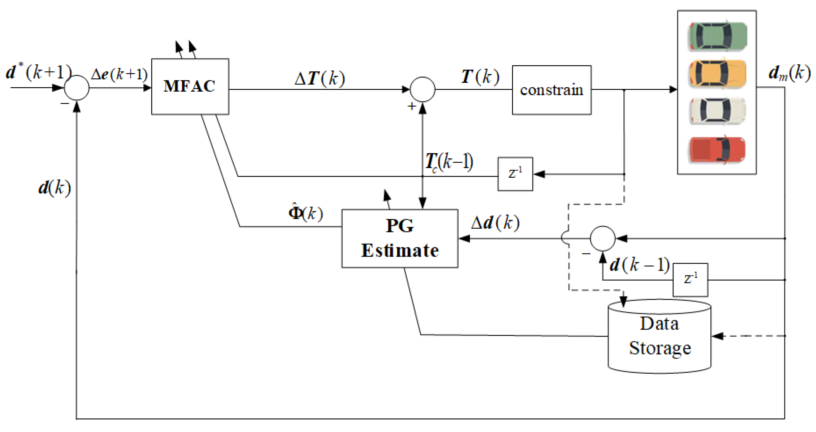
3.3. Design of cMFAC Controller

(1)

Controller design

In the vehicle queue system, information interaction can be formed between vehicles. The communication between such vehicles is represented by graph theory:

$$a_{ij}\left(k\right)=\left\{\begin{array}{c}0,\\ 1,\end{array}\right.\begin{array}{c}if\mathit{i}cannotreceivemessagesfromj\\ ificanreceivemessagesfromj\end{array},$$

(13)

similarly, the data transmission between the follower and the leader $b_{i0}$ can also be shown as above, that is,

$$b_{i0}\left(k\right)=\left\{\begin{array}{c}0,\\ 1,\end{array}\right.\begin{array}{c}if\mathit{i}canreceivemessagesfromleader\\ if\mathit{i}cannotreceivemessagesfromleader\end{array}.$$

(14)

The deviation between considered agents is defined as follows:

$$e_i\left(k\right)=d^{*}\left(k\right)-d_i\left(k\right),$$

(15)

where $d^{*}$ is the desired trajectory, and $d_i$ is the actual output of agent i. The ultimate control goal is to make all agents achieve formation control based on the expected deviation from the leader and other followers according to the locally distributed information.

Consider the following cost function of input:

$$J\left(T_i\left(k\right)\right)={\left|\sum _{j\in N_i}{a}_{i,j}\left(k\right)(d_j(k+1)-d_i(k+1))+b_i(d^{*}(k+1)-d_i(k+1))\right|}^2+\lambda {\left|\mathsf{\Delta }{T}_i\left(k\right)\right|}^2$$

(16)

where $\lambda >0$ is a weighting factor.

The input cost function (16) consists of two parts. In the first part, ${\sum }_{j\in N_i}{a}_{ij}\left(k\right)(d_j\left(k\right)$$-d_i(k+1))$ represents the local deviation between follower agent i and agents in other fields; $b_i\left(k\right)(d^{*}(k+1)-d_i(k+1))$ represents the expected deviation between agent i and virtual navigator 0, which together constitute the expected trajectory deviation. The second part is a penalty item that the control input item cannot change frequently.

To express the subsequent formula succinctly, the following definitions are given:

$${\zeta }_i\left(k\right)=\sum _{j\in N_i}{a}_{ij}\left(k\right)\left(d_j(k+1)-d_i\left(k\right)\right)+{\mathit{b}}_{i0}\left(k\right)(d^{*}(k+1)-d_i\left(k\right)).$$

(17)

Equation (18) can be obtained from $d_i(k+1)=d\left(k\right)+\mathsf{\Delta }d(k+1)$ and Equation (12).

$$\begin{array}{cc}\hfill J\left(T_i\left(k\right)\right)=& \left|\sum _{j\in N_i}{a}_{i,j}\right.\left(k\right)(d_j(k+1)-d_i\left(k\right))+b_i(d^{*}(k+1)-d_i\left(k\right))+\sum _{j\in N_i}{a}_{i,j}\left(k\right)\mathsf{\Delta }{d}_i\left(k+1\right)\hfill \\ \hfill & +b_i\mathsf{\Delta }{d}_i\left(k+1\right){|}^2+\lambda {\left|\mathsf{\Delta }{T}_i\left(k\right)\right|}^2\hfill \\ \hfill =& \left|\sum _{j\in N_i}{a}_{i,j}\right.\left(k\right)(d_j(k+1)-d_i\left(k\right))+b_i(d^{*}(k+1)-d_i\left(k\right))+\sum _{j\in N_i}{a}_{i,j}\left(k\right)\mathsf{\Phi }\left(k\right)\mathsf{\Delta }{\mathit{T}}_{\mathit{i}}\left(k\right)\hfill \\ \hfill & +b_i\mathsf{\Phi }\left(k\right)\mathsf{\Delta }{\mathit{T}}_{\mathit{i}}\left(k\right){|}^2+\lambda {\left|\mathsf{\Delta }{T}_i\left(k\right)\right|}^2.\hfill \end{array}$$

(18)

Let $\partial J\left(T_i\left(k\right)\right)$/$\partial T_i\left(k\right)=0$, the following equation can be obtained:

$$\begin{array}{cc}\hfill \partial \left(J\left(T_i\left(k\right)\right)\right)/\left(T_i\left(k\right)\right)=& 2\sum _{j\in N_i}(a_{i,j}\left(k\right)+b_i\left(k\right)){\varphi }_{\mathrm{i}1}\left(k\right)·\hfill \\ \hfill & \left|\sum _{j\in N_i}{a}_{i,j}\right.\left(k\right)(d_j(k+1)-d_i\left(k\right))+b_i\left(k\right)(d^{*}(k+1)-d_i\left(k\right))\hfill \\ \hfill & -\sum _{j\in N_i}(a_{i,j}\left(k\right)+b_i\left(k\right))\mathsf{\Phi }\left(k\right)\mathsf{\Delta }{\mathit{T}}_{\mathit{i}}\left(k\right)|-2\lambda \mathsf{\Delta }{T}_i\left(k\right)=0.\hfill \end{array}$$

(19)

By substituting Equation (17) into Equation (19), we can obtain the following equation:

$$\begin{array}{cc}\hfill & \sum _{j\in N_i}(a_{i,j}\left(k\right)+b_i\left(k\right)){\varphi }_{i1}\left(k\right)·{\zeta }_i\left(k\right)-{(\sum _{j\in N_i}(a_{i,j}\left(k\right)+b_i\left(k\right)))}^2{\varphi }_{i1}\left(k\right){\mathsf{\Phi }}_i\left(k\right)\mathsf{\Delta }{\mathit{T}}_{\mathit{i}}\left(k\right)\hfill \\ \hfill =& \sum _{j\in N_i}(a_{i,j}\left(k\right)+b_i\left(k\right)){\varphi }_{i1}\left(k\right)·{\zeta }_i\left(k\right)-{(\sum _{j\in N_i}(a_{i,j}\left(k\right)+b_i\left(k\right)))}^2{\varphi }_{i1}\left(k\right){\varphi }_{i1}\left(k\right)\mathsf{\Delta }{\mathit{T}}_{\mathit{i}}\left(k\right)\hfill \\ \hfill & -\sum _{j\in N_i}(a_{i,j}\left(k\right)+b_i\left(k\right)){\varphi }_{i1}\left(k\right)\sum _{h=2}^{\mathcal{Z}}{\widehat{\varphi }}_{i,h}\left(k\right)\mathsf{\Delta }{T}_i(k-h+1=\lambda \mathsf{\Delta }{T}_i\left(k\right)\hfill \end{array},$$

(20)

after sorting out Equation (20), Equation (21) can be obtained.

Substituting Equation (17) into Equation (16), through the optimality condition $\partial J\left(T_i\left(k\right)\right)/\partial T_i\left(k\right)=0$, the following controller can be obtained from Equation (16):

$$\mathsf{\Delta }{T}_i\left(k\right)=\frac{{\rho }_1{\widehat{\varphi }}_{i,1}\left(k\right){\zeta }_i\left(k\right)({\sum }_{j\in N_i}{a}_{i,j}+b_i)}{\lambda +{\left(({\sum }_{j\in N_i}{a}_{i,j}+b_i)\right)}^2{\widehat{\varphi }}_{i,1}{\left(k\right)}^2}-\frac{{\widehat{\varphi }}_{i,1}\left(k\right)({\sum }_{j\in N_i}{a}_{i,j}+b_i){\sum }_{h=2}^{\mathcal{Z}}{\rho }_{i,h}{\widehat{\varphi }}_{i,h}\left(k\right)\mathsf{\Delta }{T}_i(k-h+1)}{\lambda +{\left(({\sum }_{j\in N_i}{a}_{i,j}+b_i)\right)}^2{\widehat{\varphi }}_{i,1}{\left(k\right)}^2},$$

(21)

note that the output $d_i\left(k\right)$ cannot be greater than $d_{max}$, i.e.,

$$0<d_i\left(k\right)<d_{max},$$

(22)

meanwhile, the control input is under the following constraint:

$$T_{min}<T_i\left(k\right)<T_{max}.$$

(23)

After combining (20), (19) and (12), $\mathsf{\Delta }T\left(k\right)$ is subject to the following constraints:

$$\left[\begin{array}{cccc}\mathcal{R}& & & \\ & \mathcal{R}& & \\ & & \mathit{I}& \\ & & & \mathit{I}\end{array}\right]\left[\begin{array}{c}\mathsf{\Delta }{\mathit{T}}_i\left(k\right)\\ \mathsf{\Delta }{\mathit{T}}_i\left(k\right)\\ \mathsf{\Delta }{\mathit{T}}_i\left(k\right)\\ \mathsf{\Delta }{\mathit{T}}_i\left(k\right)\end{array}\right]\le \left[\begin{array}{c}{[d_{max}-d_i\left(k\right),\dots ,d_{max}-d_i\left(k\right)]}_{1\times \mathcal{Z}}^T\\ {[d_i\left(k\right),\dots ,d_i\left(k\right)]}_{1\times \mathcal{Z}}^T\\ {[T_{max}-T_i\left(k\right),\dots ,T_{max}-T_i\left(k\right)]}_{1\times \mathcal{Z}}^T\\ {[T_i\left(k\right)-T_{min},\dots ,T_i\left(k\right)-T_{min}]}_{1\times \mathcal{Z}}^T\end{array}\right].$$

(24)

$$\mathcal{R}={\left[\begin{array}{c}{{\mathsf{\Phi }}^T}_c\left(k\right)\\ ⋮\\ {{\mathsf{\Phi }}^T}_c\left(k\right)\end{array}\right]}_{\mathcal{Z}\times \mathcal{Z}}.$$

(25)

Since ${\mathsf{\Phi }}_i\left(k\right)$ in (18) is unknown, it should be evaluated to implement the controller.

Remark 4. 

${\rho }_1,{\rho }_2,\dots {\rho }_{\mathcal{Z}}\in (0,1]$ is the step-size factor, which is added to make the input smoother. The selection of λ has an important impact on the control stability, enabling it to be stable, fast, and without overshoot. Subsequent experiments will prove that the selection of λ affects the controller.

(2)

Pseudo-partial derivative estimation

Theorem 1 certifies the existence of ${\mathsf{\Phi }}_i\left(k\right)$. Since it is unknown, an estimated value is needed to replace the true value. In this study, a parameter estimation method with a symmetric control algorithm is applied to evaluate the PG value. First, the cost function for unknown ${\mathsf{\Phi }}_i\left(k\right)$ estimation is defined as

$$J\left({\mathsf{\Phi }}_i\left(k\right)\right)={∥d_i\left(k\right)-d_i(k-1)-{{\mathsf{\Phi }}_i}^T\left(k\right)\mathsf{\Delta }T(k-1)∥}^2+\mu {∥{{\mathsf{\Phi }}_i}^T\left(k\right)-{{\mathsf{\Phi }}_i}^T(k-1)∥}^2,$$

(26)

where $\mu >0$ ensures the smoothness of the algorithm.

Lemma 2 

([26] (Matrix inversion lemma)). $A,B,C,andD$ are matrices of the appropriate dimensions. If the inverse of $A$ and $C$ and ${DA}^{-1}B+C$ exists, then

$${\left[A+BCD\right]}^{-1}=A^{-1}-A^{-1}B{\left[{DA}^{-1}B+C^{-1}\right]}^{-1}{DA}^{-1}.$$

(27)

The optimal condition $\partial J\left({\mathsf{\Phi }}_i\left(k\right)\right)/\partial {\mathsf{\Phi }}_i\left(k\right)=0$ is taken, and the matrix inverse lemma [26] is used to obtain the following results:

$$\begin{array}{cc}\hfill {\widehat{\mathsf{\Phi }}}_i\left(k\right)=& {\widehat{\mathsf{\Phi }}}_i(k-1)+\frac{\eta \mathsf{\Delta }{T}_i(k-1)}{\mu +{∥\mathsf{\Delta }{T}_i(k-1)∥}^2}\hfill \\ \hfill & \times (\mathsf{\Delta }{d}_i\left(k\right)-{\widehat{\mathsf{\Phi }}}_i^T(k-1)\mathsf{\Delta }{T}_i(k-1)),\hfill \end{array}$$

(28)

where $\eta \in (0,1]$ is a step-size constant, and ${\widehat{\mathsf{\Phi }}}_i\left(k\right)$ is the estimated value of ${\mathsf{\Phi }}_i\left(k\right)$.

Remark 5. 

The cost function of input $T_i\left(k\right)$ and the cost function of parameter ${\mathsf{\Phi }}_i\left(k\right)$ have symmetrical and similar structures. It can be seen that if the control input signal in the cost function (16) and the parameter ${\mathsf{\Phi }}_i\left(k\right)$ estimation cost function (23) are interchanged, the positions of the current control input variables and parameter variables are also interchanged, and the forms of the two cost functions are identical.

To adapt the PG estimation algorithm to an actual vehicle queue and have a better capacity for tracking time-varying parameters, a reset algorithm is defined as follows:

$${\widehat{\mathsf{\Phi }}}_i\left(k\right)={\mathsf{\Phi }}_i\left(1\right),if\left|{\widehat{\mathsf{\Phi }}}_i\left(k\right)\right|\le \epsilon ,\mathrm{or}\mathsf{\Delta }{U}_i(k-1)\le \epsilon ,$$

(29)

where $\epsilon >0$ is a sufficiently small number.

Therefore, the cMFAC control scheme is obtained as follows:

$$\left\{\begin{array}{cc}\hfill & \mathsf{\Delta }{T}_i\left(k\right)=\frac{{\rho }_1{\widehat{\varphi }}_{i,1}\left(k\right){\epsilon }_i\left(k\right)({\sum }_{j\in N_i}{a}_{i,j}+b_i)}{\lambda +{\left(({\sum }_{j\in N_i}{a}_{i,j}+d_i)\right)}^2{\widehat{\varphi }}_{i,1}{\left(k\right)}^2}-\frac{{\widehat{\varphi }}_{i,1}\left(k\right)({\sum }_{j\in N_i}{a}_{i,j}+b_i){\sum }_{h=2}^{\mathcal{Z}}{\rho }_{i,\mathcal{Z}}{\widehat{\varphi }}_{i,\mathcal{Z}}\left(k\right)\mathsf{\Delta }{T}_i(k-h+1)}{\lambda +{\left(({\sum }_{j\in N_i}{a}_{i,j}+d_i)\right)}^2{\widehat{\varphi }}_{i,1}{\left(k\right)}^2},\hfill \\ \hfill & T_i\left(k\right)=T_i(k-1)+\mathsf{\Delta }{T}_i,\hfill \\ \hfill & {\zeta }_i\left(k\right)=\sum _{j\in N_i}{a}_{ij}\left(k\right)\left(d_j(k+1)-d_i\left(k\right)\right)+{\mathit{b}}_{i0}\left(k\right)(d^{*}(k+1)-d_i\left(k\right)),\hfill \\ \hfill & {\widehat{\mathsf{\Phi }}}_i\left(k\right)={\widehat{\mathsf{\Phi }}}_i(k-1)+\frac{\eta \mathsf{\Delta }{\mathit{T}}_i(k-1)}{\mu +{∥\mathsf{\Delta }{\mathit{T}}_i(k-1)∥}^2}\times (\mathsf{\Delta }{d}_i\left(k\right)-{\widehat{\mathsf{\Phi }}}_i^T(k-1)\mathsf{\Delta }{\mathit{T}}_i(k-1)),\hfill \\ \hfill & \left[\begin{array}{cccc}\mathcal{R}& & & \\ & -\mathcal{R}& & \\ & & \mathit{I}& \\ & & & \mathit{I}\end{array}\right]\left[\begin{array}{c}\mathsf{\Delta }{\mathit{T}}_i\left(k\right)\\ \mathsf{\Delta }{\mathit{T}}_i\left(k\right)\\ \mathsf{\Delta }{\mathit{T}}_i\left(k\right)\\ \mathsf{\Delta }{\mathit{T}}_i\left(k\right)\end{array}\right]\le \left[\begin{array}{c}{[d_{max},\dots ,d_{max}]}_{1\times \mathcal{Z}}^T\\ {[0,\dots ,0]}_{1\times \mathcal{Z}}^T\\ {[T_{max}-T_i\left(k\right),\dots ,T_{max}-T_i\left(k\right)]}_{1\times \mathcal{Z}}^T\\ {[T_i\left(k\right)-T_{min},\dots ,T_i\left(k\right)-T_{min}]}_{1\times \mathcal{Z}}^T\end{array}\right],\hfill \\ \hfill & \mathcal{R}={\left[\begin{array}{c}{{\mathsf{\Phi }}^T}_c\left(k\right)\\ ⋮\\ {{\mathsf{\Phi }}^T}_c\left(k\right)\end{array}\right]}_{\mathcal{Z}\times \mathcal{Z}}\hfill \end{array}\right.$$

(30a)

$$\left\{\begin{array}{cc}\hfill & {\widehat{\mathsf{\Phi }}}_i\left(k\right)={\mathsf{\Phi }}_i\left(1\right),if\left|{\widehat{\mathsf{\Phi }}}_i\left(k\right)\right|\le \epsilon ,or\left|\mathsf{\Delta }{U}_i(k-1)\right|\le \epsilon ,\hfill \\ \hfill & {\mathsf{\Phi }}_i\left(k\right)={[{\varphi }_{i,1}\left(k\right),{\varphi }_{i,2}\left(k\right)\dots ,{\varphi }_{i,\mathcal{Z}}\left(k\right)]}^T,\hfill \\ \hfill & \mathsf{\Delta }{\mathit{T}}_i\left(k\right)={\left[\mathsf{\Delta }{T}_i\left(k\right),\dots ,\mathsf{\Delta }{T}_i(k-\mathcal{Z}+1)\right]}^T.\hfill \end{array}\right.$$

(30b)

Through the output values and communication topology of the virtual navigator and other followers, the agents can travel according to the given formation and complete the required formation control. Corresponding to the fleet, vehicle queue control can be achieved by controlling the throttle/brake opening and giving the expected deviation from the pilot. The overall control system structure block diagram is shown in Figure 3, and the pseudo-code of the control flow is shown in Algorithm 1.

Algorithm 1: Pseudocode of the cMFAC Algorithm.

While k<max_execution time do    Calculate the distance difference e(k) between the follow vehicle and the leader vehicle    Calculate the next time input T(k) according(21)    if T(k) < $T_{max}$ (k)       Perform constraint processing    End if    Input the T(k) at this time into the following vehicle to obtain the output d(k + 1)    Calculate the Δd(k + 1)    Estimate the pseudo derivative Φ(k + 1) according(28)    Storage the Φ(k + 1), T(k) and d(k + 1) End

Lemma 3 

([27]). Let

$$X=\left[\begin{array}{cccc}{x}_1& x_2& \dots & \begin{array}{cc}{x}_{\mathcal{Z}-1}& x_{\mathcal{Z}}\end{array}\\ 1& 0& \dots & \begin{array}{cc}0& 0\end{array}\\ 0& 1& \dots & \begin{array}{cc}0& 0\end{array}\\ \begin{array}{c}⋮\\ 0\end{array}& \begin{array}{c}⋮\\ 0\end{array}& \begin{array}{c}⋮\\ \dots \end{array}& \begin{array}{c}\begin{array}{cc}⋮& ⋮\end{array}\\ \begin{array}{cc}1& 0\end{array}\end{array}\end{array}\right],$$

if ${\sum }_{h=1}^{\mathcal{Z}}\left|x_i\right|<1$, $s\left(X\right)<1$. where $s(·)$ is the spectral radius.

Theorem 2. 

A class of multiagent systems with data compensation is considered. When Assumptions 1–3 are met, the input and output of the system do not exceed the upper and lower limits. An appropriate ${\rho }_1$ is selected to meet the following conditions:

$${\rho }_1<\frac{1}{{max}_{i=1\dots ,N}{\sum }_{j=1}^N{a}_{ij}+b_i}$$

(31)

Then, there must be a suitable $\lambda$ so that when $\lambda >{\lambda }_{min}$, the expected trajectory deviation $e\left(k\right)={\left[e_1\left(k\right)e_2\left(k\right)\dots e_N\left(k\right)\right]}^T$ meets the following conditions:

$$\underset{k\to \infty }{lim}∥\mathsf{\Delta }T(k+1)∥\le p$$

(32)

$$\underset{k\to \infty }{lim}∥e(k+1)∥\le \upsilon$$

(33)

where p and $\upsilon$ are small positive numbers.

Proof. 

See Appendix A. □

4. Experimental Simulation

This section consists of two parts. Section 4.1 discusses numerical simulations using MATLAB 2020b to certify the effectiveness of the cMFAC algorithm for MAS control. In Section 4.2, CarSim is used for semi-physical experiments to certify the effectiveness of the control strategy for multivehicle collaborative control.

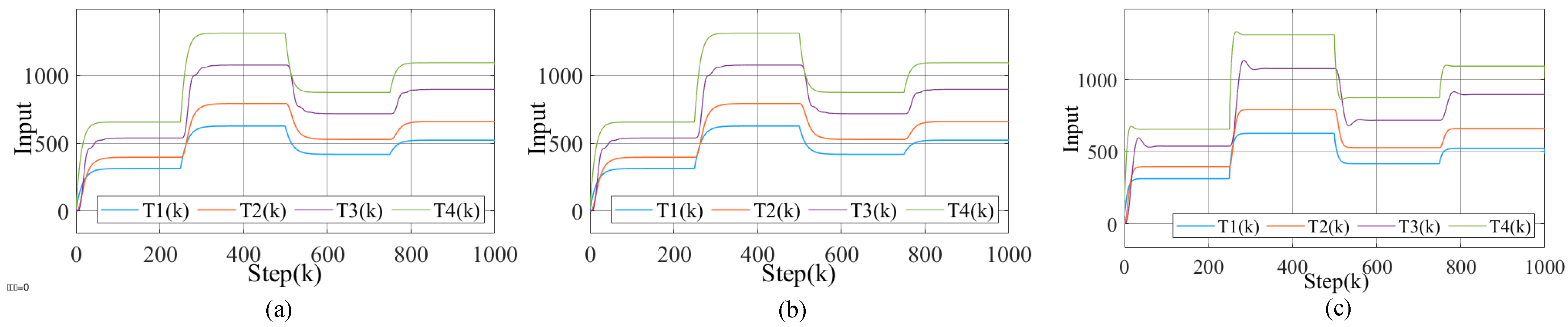
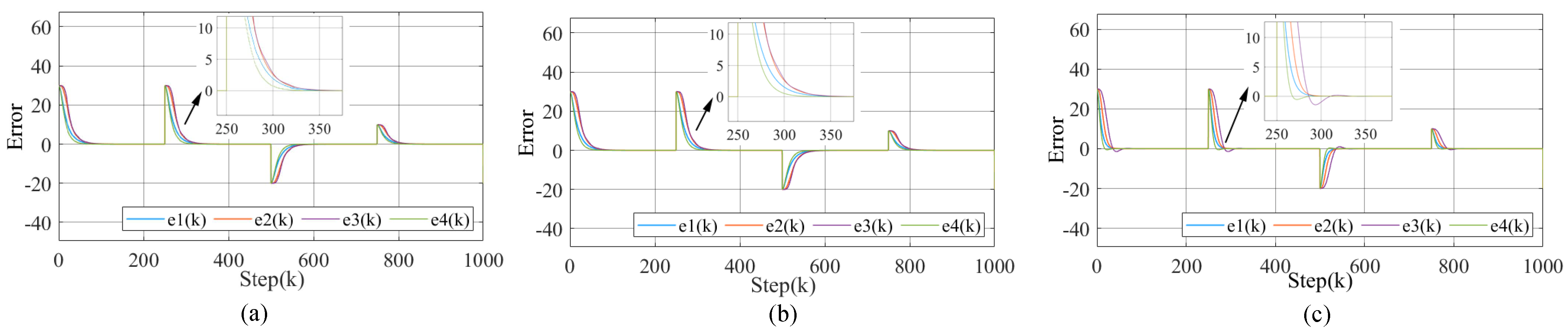
4.1. Numerical Simulation Comparison

To certify the effectiveness of the above cMFAC algorithm on the MAS system, numerical simulations are discussed in this part. Numerical simulations included three experiments. PID and cMFAC were, respectively, used for comparative tests to prove the convergence performance of cMFAC; MFAC and cMFAC were used for comparative tests to prove the constraint performance; and cMFAC convergence performance under different $\lambda$ values was evaluated to investigate the influence of $\lambda$ on cMFAC. It is worth noting that the MAS in this part is a SISO system, and the given agent dynamics were only used to generate I/O data, and the design of the controller was not considered.

(1)

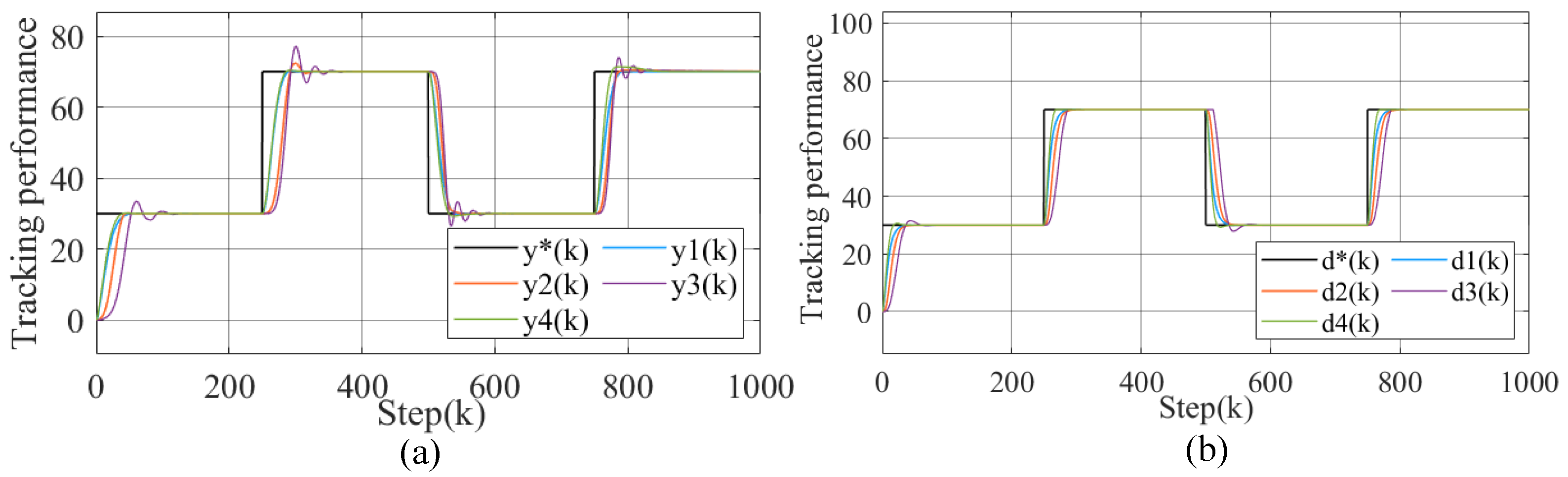
Square wave trajectory tracking

The first experiment considered the ability to track the desired value in the case of a square wave, and the cMFAC and PID effects for MAS control were tested. The PID algorithm is as follows:

$$d_i\left(k\right)=K_{p}T\left(k\right)+K_i{\sum }_0^{k}e\left(k\right)+K_d(e\left(k\right)-e(k-1))$$

(34)

where $K_p$ is the proportional coefficient, $K_i$ is the integral coefficient, and $K_d$ is the differential coefficient.

The data transmission between multiple agents is shown in Figure 4.

As shown in Figure 4, vehicle 0 was the lead vehicle, and only vehicle 1 could receive a message from vehicle 0. The nonlinear discrete MAS was composed of successively following agents, and the topology shows that the structure is strongly connected. The weighted adjacency matrix $\mathcal{A}$ can be written as

$$\mathcal{A}=\left[\begin{array}{cccc}0& 0& 0& 1\\ 1& 0& 0& 0\\ 1& 1& 0& 0\\ 0& 0& 1& 0\end{array}\right].$$

(35)

Consider the following constant expectations:

$$d^{*}\left(k\right)=\left\{\begin{array}{c}30\\ 60\\ 40\\ 50\end{array}\right.\begin{array}{c}0<k\le 250\\ 250<k\le 500\\ 500\le k<750\\ 750\le k<1000\end{array}.$$

(36)

A group of discrete SISO MASs with heterogeneous nonaffine nonlinearity can be described as follows:

$$\left\{\begin{array}{c}Agent1:y_1(k+1)=0.003u_1\left(k\right)+0.003u_1(k-1)\hfill \\ +1.95y_1\left(k\right)-0.951y_1(k-1)\hfill \\ Agent2:y_2(k+1)=0.0046u_2\left(k\right)+0.0045u_2(k-1)\hfill \\ +1.935y_2\left(k\right)-0.936y_2(k-1)\hfill \\ Agent3:y_3(k+1)=0.0124u_3\left(k\right)+0.01107u_3(k-1)\hfill \\ +1.702y_3\left(k\right)-0.704y_3(k-1)\hfill \\ Agent4:y_4(k+1)=0.0056u_4\left(k\right)+0.0055u_4(k-1)\hfill \\ +1.935y_4\left(k\right)-0.936y_4(k-1).\hfill \end{array}\right.$$

(37)

The main parameters and initial values of the PID and cMFAC controllers are shown in

Table 1. Parameter settings of the two control methods.

Algorithm	Parameter Settings
cMFAC	$\eta =1.45$, $\mu =0.8$, $\lambda =1.2$, $\rho =1$, ${\varphi }_1\left(1\right)={\varphi }_2\left(1\right)={\varphi }_3\left(1\right)=0.1$, $\mathcal{Z}$=3
Z-N-PID	$K_p=2.2$, $T_i=1.2$, $T_d=0$
GWO-PID	$K_p=2.194$, $T_i=1.181$, $T_d=0$

. The cMFAC parameters were selected according to the characteristics of the MFAC controller parameters and a large number of experiments. The PID parameters were estimated by using the gray wolf optimization (GWO) algorithm and Z–N turning, respectively. [28]. The simulation time was set to 1000 steps, and the simulation results are shown in Figure 5, Figure 6 and Figure 7.

According to Figure 5, Figure 6 and Figure 7, the PID and cMFAC can both complete the MAS control task. However, we can see that the cMFAC has a better tracking effect and control speed, and the convergence speed of the search agent is faster.

To demonstrate the performance of the cMFAC algorithm under constraints, it was compared with the traditional MFAC algorithm. The controlled object still adopted Equation (34). The data transmission between multiple agents is shown in Figure 4. The expected values are as follows:

$$d^{*}\left(k\right)=\left\{\begin{array}{c}30\\ 70\\ 30\\ 70\end{array}\right.\begin{array}{c}0<k\le 250\\ 250<k\le 500\\ 500\le k<750\\ 750\le k<1000.\end{array}$$

(38)

The conventional MFAC controller is as follows:

$${\widehat{\mathsf{\Phi }}}_i\left(k\right)={\widehat{\mathsf{\Phi }}}_i(k-1)+\frac{\eta \mathsf{\Delta }{T}_i(k-1)}{\mu +{∥\mathsf{\Delta }{T}_i(k-1)∥}^2}\times (\mathsf{\Delta }{d}_i\left(k\right)-{\widehat{\mathsf{\Phi }}}_i^T(k-1)\mathsf{\Delta }{T}_i(k-1))$$

(39)

$$\begin{array}{cc}\hfill \mathsf{\Delta }{T}_i\left(k\right)=& \frac{{\rho }_1{\widehat{\varphi }}_{i,1}\left(k\right){\epsilon }_i\left(k\right)({\sum }_{j\in N_i}{a}_{i,j}+d_i)}{\lambda +{\left(({\sum }_{j\in N_i}{a}_{i,j}+d_i)\right)}^2{\widehat{\varphi }}_{i,1}{\left(k\right)}^2}\hfill \\ \hfill & -\frac{{\widehat{\varphi }}_{i,1}\left(k\right)({\sum }_{j\in N_i}{a}_{i,j}+d_i){\sum }_{h=2}^{\mathcal{Z}}{\rho }_{i,h}{\widehat{\varphi }}_{i,h}\left(k\right)\mathsf{\Delta }{T}_i(k-h+1)}{\lambda +{\left(({\sum }_{j\in N_i}{a}_{i,j}+d_i)\right)}^2{\widehat{\varphi }}_{i,1}{\left(k\right)}^2}\hfill \end{array}$$

(40)

$${\widehat{\mathsf{\Phi }}}_i\left(k\right)={\mathsf{\Phi }}_i\left(1\right),if\left|{\widehat{\mathsf{\Phi }}}_i\left(k\right)\right|\le \epsilon ,or\left|\mathsf{\Delta }{U}_i(k-1)\right|\le \epsilon$$

(41)

The parameters initial values of the MFAC and cMFAC controllers are shown in

Table 2. Parameter settings of the two control methods.

Algorithm	Parameter Settings
MFAC	$\eta =1.45$, $\mu =0.8$, $\lambda =1.2$, $\rho =1$, ${\varphi }_1\left(1\right)={\varphi }_2\left(1\right)={\varphi }_3\left(1\right)=0.1$, $\mathcal{Z}$ = 3
cMFAC	$\eta =1.45$, $\mu =0.8$, $\lambda =1.2$, $\rho =1$, ${\varphi }_1\left(1\right)={\varphi }_2\left(1\right)={\varphi }_3\left(1\right)=0.1$, $\mathcal{Z}$ = 3, $d_{max}$ = 70, $T_{max}$ = 1600, $T_{min}=0$

. The cMFAC and MFAC parameters were selected according to the characteristics of the MFAC controller parameters and a large number of experiments. The upper limit of the output was 70, the lower limit was 0, the upper limit of the input was 1600, and the lower limit was 0. The simulation step was set to 1000 steps, and the simulation results are shown in Figure 8 and Figure 9.

Figure 8 and Figure 9 show that both control algorithms can complete the control task. However, the input and output of the traditional MFAC obviously exceed the constraint value, while the proposed cMFAC can effectively constrain the input and output without interfering with the control effect.

(2)

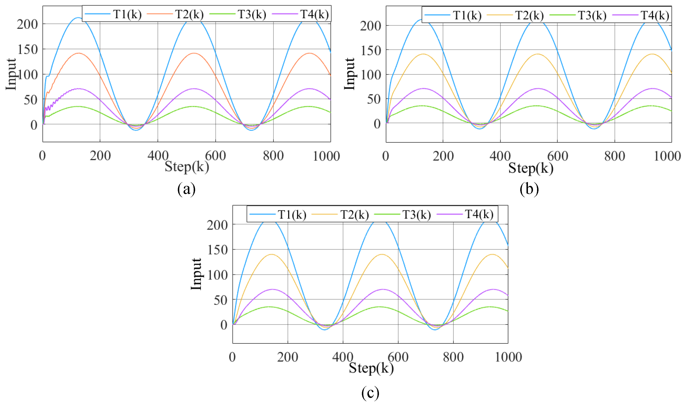
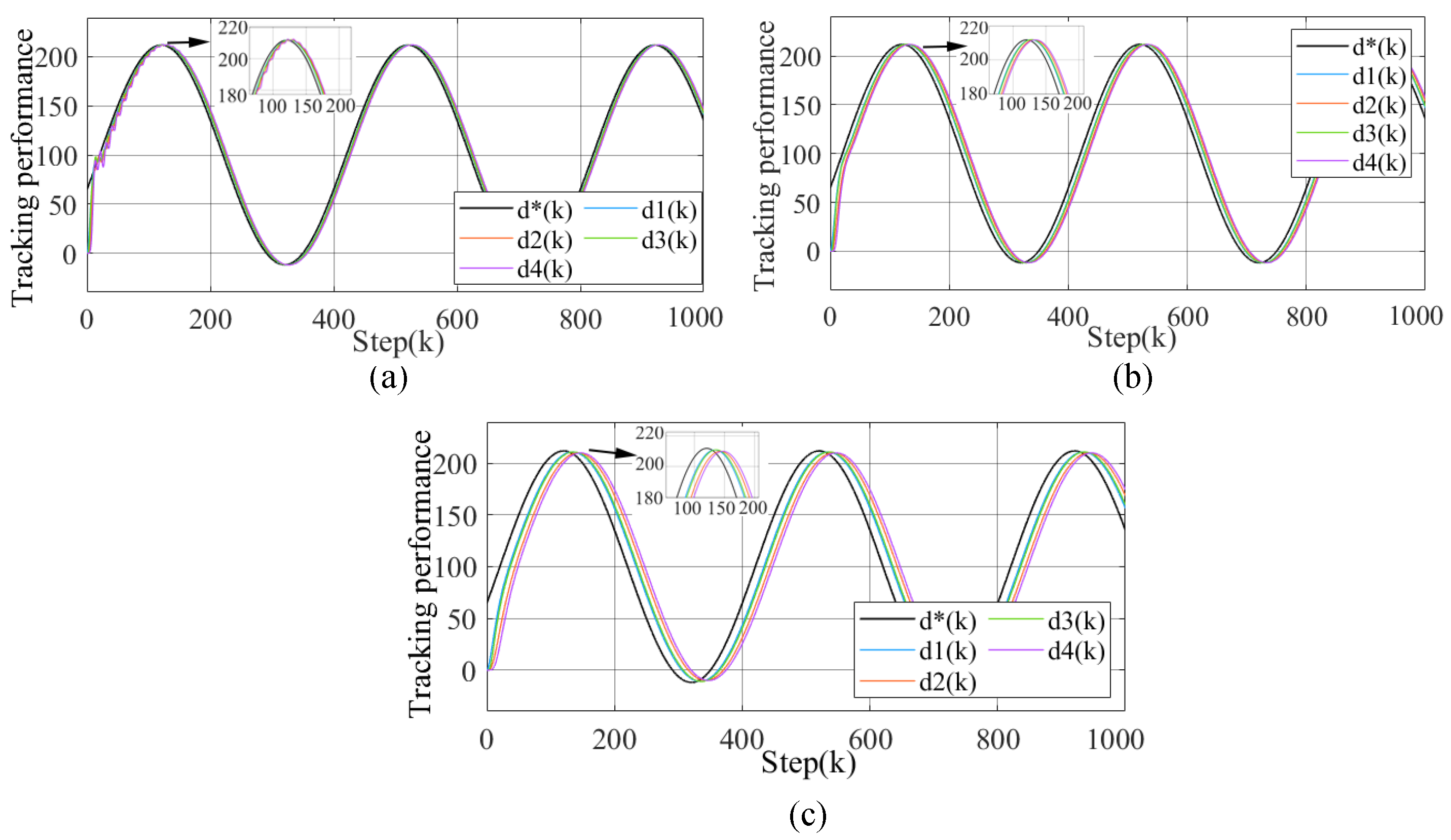
Time-varying trajectory tracking

The second experiment considered the ability to track the desired value under the time-varying trajectory in the case of packet loss and tested the influence of different $\lambda$ values on the control effect. The expected values of the system are as follows:

$$\begin{array}{c}{d}^{*}\left(k\right)=100+100\sin (k\pi /200-\pi /4)\hfill \\ +50\cos (k\pi /200-\pi /4).\hfill \end{array}$$

(42)

The data transmission between multiple agents is shown in Figure 10.

As shown in Figure 10, vehicle 0 was the lead vehicle, and only vehicle 1 could receive a message from vehicle 0. The nonlinear discrete MAS was composed of four agents, and the topology shows that the structure is strongly connected. The weighted adjacency matrix $\mathcal{A}$ can be written as follows:

$$A=\left[\begin{array}{cccc}0& 0& 0& 1\\ 1& 0& 1& 0\\ 1& 0& 0& 0\\ 0& 1& 0& 0\end{array}\right].$$

(43)

In this experiment, the values of $\lambda$ were 5, 10, and 20. The initial values of the cMFAC controller are shown as follows: $\eta =1$, $\mu =0.8$, $\rho =0.3$, ${\varphi }_1\left(1\right)={\varphi }_2\left(1\right)={\varphi }_3\left(1\right)=0.5$, $\mathcal{Z}$ = 3. The cMFAC parameters were selected according to the characteristics of the MFAC controller parameters and a large number of experiments. The simulation time was set to 1000 steps, and the simulation results are shown in Figure 11, Figure 12 and Figure 13.

Figure 11, Figure 12 and Figure 13 show that the value of $\lambda$ has a great impact on the control effect. If the value of $\lambda$ is too small ($\lambda$ = 5), the system will vibrate. If the value of $\lambda$ is too large ($\lambda$ = 20), the convergence speed of the system will be slower, and the adjustment time will be longer. Therefore, it is important to reasonably select $\lambda$ for the proposed algorithm.

4.2. CarSim Simulation

This part discusses using the CarSim platform to verify the control effect of the proposed cMFAC algorithm on multiple vehicles. CarSim is a simulation platform specifically designed for vehicle dynamics. It has the advantages of multidisciplinary system simulation. It is mainly used to simulate the dynamic performance, braking performance, handling stability, and other performance indicators of the whole vehicle. The host is based on the Windows operating system, equipped with an AMD Ryzen 7 4800H eight-core processor and 16 GB of memory. In this experiment, the dynamic models of three vehicles were added as the controlled MASs, and the final control objectives were as follows:

(1).

The speed of all vehicles would reach the speed of the leader vehicle to ensure that the speed difference tends to zero;

(2).

The positions of all vehicles would form a fixed vehicle spacing in a given way and ensure spacing safety.

Three vehicles were selected as experimental objects for simulation, namely, vehicle 1, vehicle 2, and vehicle 3, as shown in Figure 14. The specific parameters of the three vehicles are shown in

Table 3. Detailed parameters of the three vehicles.

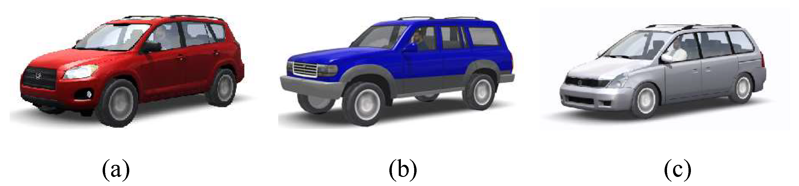
Vehicle	1	2	3
Total mass	1430 kg	1590 kg	1800 kg
Engine power	150 kW	200 kW	150 kW
Brake torque	450 N·m	500 N·m	450 N·m
Length	2650 mm	2950 mm	3000 mm
Windward area	3.06 m2	3.38 m2	3.18 m2
Road resistance coefficient	0.15	0.15	0.15
Air density	1.29	1.29	1.29
slope	-	-	-

.

The running time of the vehicle was set to 120 s. Due to driving in the city, the desired vehicle speed track was designed as follows:

$$V_d\left(k\right)=\left\{\begin{array}{c}40\\ \begin{array}{c}50\\ 70\end{array}\end{array}\right.\begin{array}{c}k\le 40\\ \begin{array}{c}40<k\le 80\\ 80<k\le 120.\end{array}\end{array}$$

(44)

The controller parameters were set as shown in

Table 4. Related parameters of the IOC cMFAC algorithm under the CarSim semi-physical simulation experiment.

Parameter	Value	Parameter	Value
$\rho$	0.9	$\eta$	0.6
$\lambda$	6.5	$\mu$	1
${\varphi }_1\left(1\right){\varphi }_2\left(1\right){\varphi }_3\left(1\right)$	0.5	$\mathcal{Z}$	3

.

The input constraint of the vehicle was imposed by driving under the speed constraint, and the vehicle speed did not exceed 75 km/h. Vehicle 1 was the leader vehicle, vehicle 2 received the information from vehicle 1, and vehicle 3 received the information from vehicle 2. The simulation scene was a straight road. The simulation results are shown in Figure 15, Figure 16 and Figure 17. They are the speed output curve, the output torque, i.e., the control input, and the driving distance of each vehicle, respectively.

Figure 15 and Figure 16 show that during 0–20 s, 40–50s, and 80–90 s, due to the constant acceleration process, the output torque increased, and the speed of the following vehicles had a certain error with the leader, but the following vehicles could keep up with the leader’s speed and maintain the same speed, and the speed of the last two vehicles did not exceed the set constraint value. Figure 16 shows that since the vehicle behind accelerated from 0, the early control input continuously increased to adjust the speed. In the constant speed stage, due to the resistance factor, the torque did not always remain unchanged but fluctuated within the controllable range.

As shown in Figure 17, in the fleet system, all three vehicles had consistent positions. After starting and accelerating, the distance between vehicles was always kept at the set distance. Therefore, the designed cMFAC controller has good application in longitudinal multivehicle cooperative control systems.

5. Conclusions

This manuscript presents a new cMFAC algorithm for multivehicle cooperative control. In the cMFAC method, first, based on a PFDL data model, a new partial form dynamic linearization technique was used to convert the multivehicle collaborative system into a virtual data model to estimate the time-varying parameter PG. Then the estimated PG was used to estimate the output value and set input and output constraints. The estimation cost function of PG and the estimation cost function of the input value had a symmetric similar structure. It is worth noting that in the process of using this method to design the controller, no accurate controlled object model was needed, and only I/O measurements were required to complete the control task. The convergence and stability of the algorithm were mathematically proven. In addition, CarSim and MATLAB were used for joint simulation to verify the applicability of the algorithm in a multivehicle collaborative system.

References

- Wei, Y.; Avcı, C.; Liu, J.; Belezamo, B.; Aydın, N.; Li, P.T.; Zhou, X. Dynamic programming-based multi-vehicle longitudinal trajectory optimization with simplified car following models. Transp. Res. Part B Methodol. 2017, 106, 102–129. [Google Scholar] [CrossRef]
- Wang, Z.; Bian, Y.; Shladover, S.E.; Wu, G.; Li, S.E.; Barth, M.J. A survey on cooperative longitudinal motion control of multiple connected and automated vehicles. IEEE Intell. Transp. Syst. Mag. 2019, 12, 4–24. [Google Scholar] [CrossRef] [Green Version]
- Hu, L.; Zhou, X.; Zhang, X.; Wang, F.; Li, Q.; Wu, W. A review on key challenges in intelligent vehicles: Safety and driver-oriented features. IET Intell. Transp. Syst. 2021, 15, 1093–1105. [Google Scholar] [CrossRef]
- Xie, H.; Xiao, P. Cooperative Adaptive Cruise Algorithm Based on Trajectory Prediction for Driverless Buses. Machines 2022, 10, 893. [Google Scholar] [CrossRef]
- Kneissl, M.; Madhusudhanan, A.K.; Molin, A.; Esen, H.; Hirche, S. A multi-vehicle control framework with application to automated valet parking. IEEE Trans. Intell. Transp. Syst. 2020, 22, 5697–5707. [Google Scholar] [CrossRef]
- Sancar, F.E.; Fidan, B.; Huissoon, J.P.; Waslander, S.L. MPC based collaborative adaptive cruise control with rear end collision avoidance. In Proceedings of the 2014 IEEE Intelligent Vehicles Symposium Proceedings, Dearborn, MI, USA, 8–11 June 2014; IEEE: New York, NY, USA, 2014; pp. 516–521. [Google Scholar]
- Alam, A.; Mårtensson, J.; Johansson, K.H. Experimental evaluation of decentralized cooperative cruise control for heavy-duty vehicle platooning. Control Eng. Pract. 2015, 38, 11–25. [Google Scholar] [CrossRef]
- Xu, L.; Zhuang, W.; Yin, G.; Bian, C. Distributed formation control of homogeneous vehicle platoon considering vehicle dynamics. Int. J. Automot. Technol. 2019, 20, 1103–1112. [Google Scholar] [CrossRef]
- Wen, S.; Guo, G. Control of leader-following vehicle platoons with varied communication range. IEEE Trans. Intell. Veh. 2019, 5, 240–250. [Google Scholar] [CrossRef]
- Wang, J.; Luo, X.; Wang, L.; Zuo, Z.; Guan, X. Integral sliding mode control using a disturbance observer for vehicle platoons. IEEE Trans. Ind. Electron. 2019, 67, 6639–6648. [Google Scholar] [CrossRef]
- Guo, K.; Jiang, J.; Li, Z. Diffusion and persistence of rotor/stator synchronous full annular rub response under weak random perturbations. J. Vib. Eng. Technol. 2020, 8, 599–611. [Google Scholar] [CrossRef]
- Safonov, M.G.; Tsao, T.C. The unfalsified control concept and learning. IEEE Trans. Autom. Control 1997, 42, 843–847. [Google Scholar] [CrossRef]
- Campestrini, L.; Eckhard, D.; Chia, L.A.; Boeira, E. Unbiased MIMO VRFT with application to process control. J. Process Control 2016, 39, 35–49. [Google Scholar] [CrossRef]
- Li, M.; Zhu, Y.; Yang, K.; Yang, L.; Hu, C.; Mu, H. Convergence rate oriented iterative feedback tuning with application to an ultraprecision wafer stage. IEEE Trans. Ind. Electron. 2018, 66, 1993–2003. [Google Scholar] [CrossRef]
- Sun, X.; Jin, Z.; Chen, L.; Yang, Z. Disturbance rejection based on iterative learning control with extended state observer for a four-degree-of-freedom hybrid magnetic bearing system. Mech. Syst. Signal Process. 2021, 153, 107465. [Google Scholar] [CrossRef]
- Liu, S.; Hou, Z.; Tian, T.; Deng, Z.; Li, Z. A novel dual successive projection-based model-free adaptive control method and application to an autonomous car. IEEE Trans. Neural Netw. Learn. Syst. 2019, 30, 3444–3457. [Google Scholar] [CrossRef]
- Chu, W.; Guan, X.; Cai, Z.; Gao, L. Real-time volume control for interactive network traffic replay. Comput. Netw. 2013, 57, 1611–1629. [Google Scholar] [CrossRef]
- Zhang, H.; Zhou, J.; Sun, Q.; Guerrero, J.M.; Ma, D. Data-driven control for interlinked AC/DC microgrids via model-free adaptive control and dual-droop control. IEEE Trans. Smart Grid 2015, 8, 557–571. [Google Scholar] [CrossRef] [Green Version]
- Chi, R.-H.; Hou, Z.-S. A model-free periodic adaptive control for freeway traffic density via ramp metering. Acta Autom. Sin. 2010, 36, 1029–1033. [Google Scholar] [CrossRef]
- Pang, Z.H.; Liu, G.P.; Zhou, D.; Sun, D. Data-based predictive control for networked nonlinear systems with network-induced delay and packet dropout. IEEE Trans. Ind. Electron. 2015, 63, 1249–1257. [Google Scholar] [CrossRef]
- Devi, V.S.; Ravi, T.; Priya, S.B. Cluster based data aggregation scheme for latency and packet loss reduction in WSN. Comput. Commun. 2020, 149, 36–43. [Google Scholar] [CrossRef]
- Sun, Z.; Tao, R.; Xiong, N.; Pan, X. CS-PLM: Compressive sensing data gathering algorithm based on packet loss matching in sensor networks. Wirel. Commun. Mob. Comput. 2018, 2018, 5131949. [Google Scholar] [CrossRef]
- Zhichao, C.; Ruju, Z. Classification of Irreducible Z+ Modules of a Z+ Ring Using Matrix Equations. Symmetry 2022, 14, 2598. [Google Scholar]
- Hou, Z.; Jin, S. A novel data-driven control approach for a class of discrete-time nonlinear systems. IEEE Trans. Control Syst. Technol. 2010, 19, 1549–1558. [Google Scholar] [CrossRef]
- He, S.; Fang, H.; Zhang, M.; Liu, F.; Luan, X.; Ding, Z. Online policy iterative-based H∞ optimization algorithm for a class of nonlinear systems. Inf. Sci. 2019, 495, 1–13. [Google Scholar] [CrossRef]
- Yue, S.; Li, Y.; Wei, A.; Zhao, J. An Efficient Method for Split Quaternion Matrix Equation X − Af(X)B = C. Symmetry 2022, 14, 1158. [Google Scholar] [CrossRef]
- Amiri, I.; Ali, J. Simulation of the single ring resonator based on the Z-transform method theory. Quantum Matter 2014, 3, 519–522. [Google Scholar] [CrossRef]
- Zhou, N.; Xia, Y. Coordination control design for formation reconfiguration of multiple spacecraft. IET Control Theory Appl. 2015, 9, 2222–2231. [Google Scholar] [CrossRef]