1. Introduction
The gamma process has been considered as an important approach to deal with the stochastic modeling of degradation processes. The reason of this is because this process has important characteristics that allows to describe a broad variety of phenomenons, in which the degradation processes are included [
1]. The asymmetrical form of the distribution allows to describe increasing degradation process, but as the shape parameter of the distribution is greater it tends to be symmetrical, which allows to extend the applicability of the model. Several applications in diverse scientific areas can be found in the literature, in which the main objective is to obtain estimations about the reliability and quality of products and systems. For example, Park and Kim [
2] considered the gamma process to model the degradation process of photovoltaic modules with the objective of estimating the lifetime of the devices. Yuan et al. [
3] defined a modeling scheme based on the gamma process and a Bayesian approach to determine a maintenance program for the corrosion in the primary cooling piping system of a nuclear plant. Iervolino et al. [
4] modeled the degradation process of the simple single degree of freedom elastic-perfectly-plastic structures due to earthquakes with the objective of defining a life-cycle structural assessment. Qiu and Cui [
5] defined optimal abort policies for unmanned aerial vehicles based on the gamma process. Sun et al. [
6] modeled the sealing performance of gas steering engine rubber O-rings based on a gamma process, and an accelerated degradation test was performed based on different temperatures. The gamma process has also been used to model different characteristics of light-emitting diodes (LEDs). For example, Park and Kim [
7] considered the light flux and chromaticity of LED lamps as characteristics to be modeled, and they estimated the median life of the device under test and defined a warranty life based on the 2.5% percentile. Furthermore, Ibrahim et al. [
8] modeled the luminous flux degradation of phosphor-converted white LEDs considering a temperature accelerated degradation test to estimate their lifetime. Meanwhile, Fan et al. [
9] considered a moisture accelerated degradation test to study the degradation process of the silicon encapsulant of a LED packaging, with the objective of estimate the reliability of the devices. On the other hand, Lin et al. [
10] considered the gamma process to model the voltage-discharge curves of the cycle aging of rechargeable batteries, the authors considered a two phase gamma process with a change-point to estimate the remaining useful life of the devices. Hu et al. [
11] also estimated the remaining useful for a fatigue crack length dataset of an A2017-T4 aluminum alloy. Mo et al. [
12] used the gamma process to model the strength degradation process of the shaft end of wind turbines by considering the stress–strength model; the reliability was assessed with the first-passage time distribution of the process. Zhang et al. [
13] proposed a Bayesian approach to estimate the reliability of a multi-component system under a stress-strength model by considering a Marshall–Olkin Weibull model. M’Sabah et al. [
14] used the gamma process to determine an effective maintenance plan based on the degradation process of a motor pump bearing. Finally, a general application was proposed by Zhang et al. [
15], in which they defined a reliability demonstration plan based on optimal accelerated degradation tests.
These previously discussed applications have different characteristics that imply to consider variations in the structure the gamma process model. One important aspect is that there may be a unit-to-unit variability among the devices under test [
16], which may be due to the differences in material composition and environmental conditions. This variability needs to be incorporated in the modeling such that it is possible to obtain accurate reliability estimations. Specifically, this unit-to-unit variability can be incorporated by considering random effects, which consists in determining that one of the parameters of the stochastic process is a random variable that can be estimated for every unit under test. For the gamma process, there are several published works in the literature that consider random effects under different scenarios. Normally, the random effects are incorporated by defining that the scale parameter is a random variable; for example, Wang et al. [
17] studied the gamma process with random scale to determine generalized confidence intervals for the shape parameter of the process. Meanwhile, Liu et al. [
18] proposed an interval degradation model approach for the random scale gamma process. Wang et al. [
19] also considered a random scale in the gamma process to model a degradation process under an accelerated degradation test. They proposed a Bayesian estimation approach to obtain the parameters of the model. Liu et al. [
20] considered a Bayesian model averaging approach to combine this model with the inverse Gaussian process. Wang et al. [
21] considered the same random effects gamma process model combined with isotonic regression to estimate the remaining useful of bearings and also to determine an optimal maintenance time for the device under test. On the other hand, Guida and Penta [
22] modeled a fatigue crack growth data by also considering the Paris law. Giorgio et al. [
23] proposed a transformed gamma process that considers two functions as the age function and the state function to model non-independent degradation measurements that are observed over disjoint time intervals. They also considered the scale parameter to introduce unit-to-unit variability. Rodríguez-Picón et al. [
24] studied different scenarios to introduce random effects in the gamma process, these scenarios considered that any of the parameters of the gamma process can be considered as random.
Another aspect can be found when several characteristics of a device may be of interest and can be simultaneously observed, which denotes the need to consider a multivariate modeling. The gamma process with random scale, can be considered to model the marginal distributions by considering copula functions [
25,
26]. Furthermore, the gamma process with random scale has been considered to determine the optimal design of degradation tests. Duan and Wang [
27] and Tsai et al. [
28] developed optimal degradation tests considering design variables as sample size, measurement frequency, and number of measurements to minimize the asymptotic variance of the estimated reliability and the 100p-th percentile. On the other hand, as the gamma process with random scale has a complex form, alternative approaches for the estimation of parameters has been proposed in the literature. In addition to the maximum likelihood estimation (MLE) and Bayesian approach, Ye et al. [
29] proposed a semi-parametric estimation approach based on the expectation-maximization (EM) algorithm, while Wang et al. [
19] proposed a semi-parametric pseudo-likelihood approach based on the pool adjacent violators algorithm to estimate the parameters of the gamma process with random scale. Other approaches can be considered to model the effect of dynamic operating environmental conditions in a system. For example, Luo et al. [
30] presented an approach that considers to model the effects as the cumulative hazard function of the exponential dispersion process and also considered lifetime ordering constraints.
All of the previously discussed works present different schemes for the application of the gamma process with random scale. However, this model only considers one source of variability in the scale parameter. In reality, a product may have multiple sources of variability that affects its performance, such as specific characteristics of the product and environmental conditions. Rodríguez-Picón et al. [
31], presented a gamma process with two sources of variation, specifically by considering that both the threshold and the initial level of degradation are random variables. The modeling approach considered to obtain the subtraction of both random variables based on a deconvolution operation. As this operation results in a complex form, it was considered to obtain an approximation by considering the fast Fourier algorithm. Then the approximation was fitted to different distributions to then characterize the first-passage time distribution of the process via numerical integration. In this paper, we improve several aspects of this proposed approach and extend the consideration of an additional source of variation. In the first instance, the proposed model in this paper also considers that the threshold level and the initial level of degradation are random variables. In addition to these two sources of variability, we consider the scale parameter of the gamma process as a source of variation. This is an important consideration, as unit-to-unit variability may be expected to be present in the degradation process of most products, as has been discussed in the previously published works. Furthermore, an important improvement of the proposed approach relies on that the subtraction of the random threshold and the random initial level are obtained based on a convolution operation instead of a deconvolution. This consideration allows to directly obtain the subtraction of these random variables to then be incorporated into the gamma process model with random scale, instead of using an approximation that then is used to be fitted to other distributions.
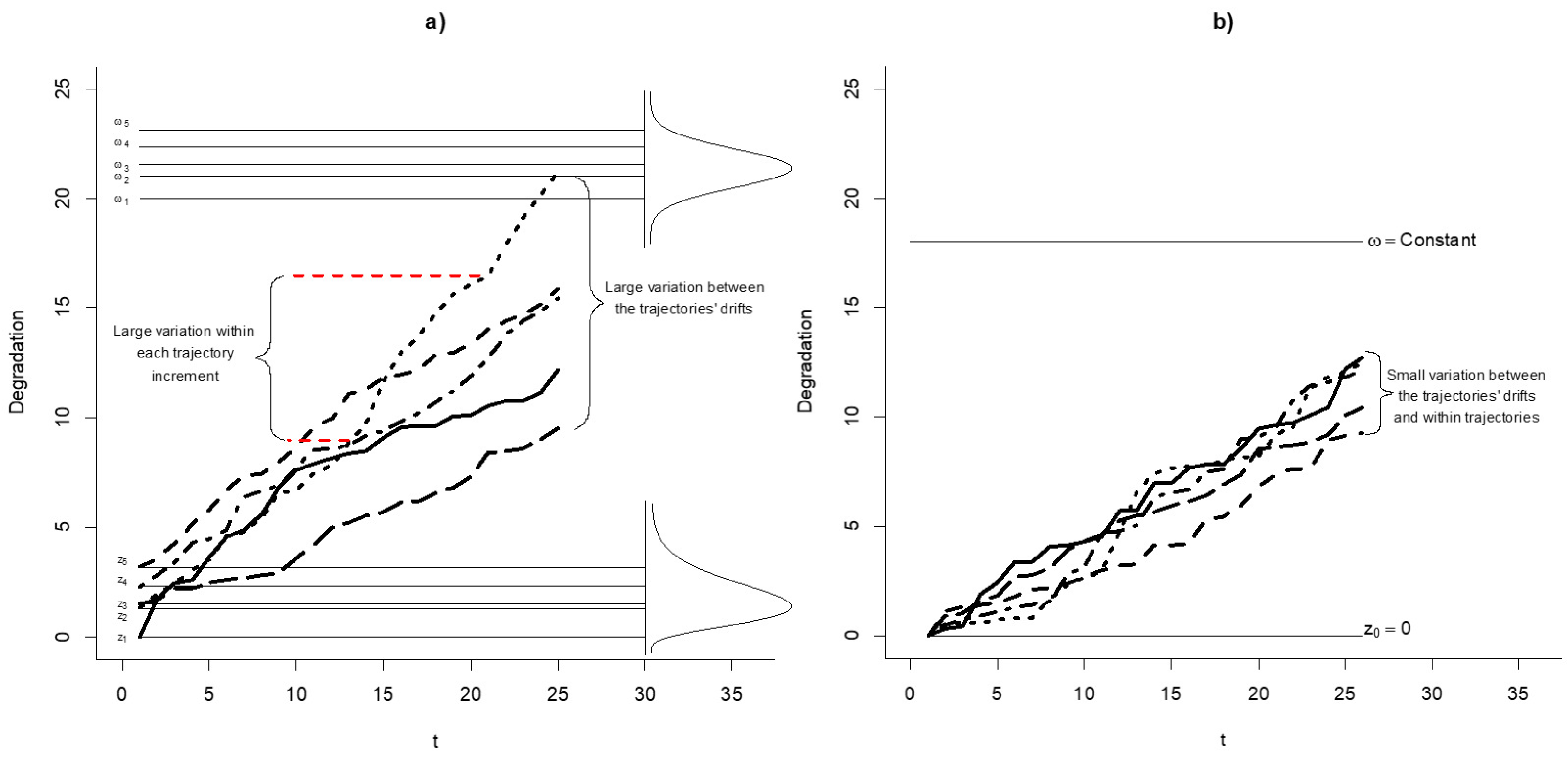
The three sources of variation are illustrated in
Figure 1, where five trajectories from a gamma process were simulated. Specifically, it can be noted in
Figure 1a that both the initial level of degradation and the threshold are different for every trajectory, which accounts for two sources of variation. For some devices, the initial level of degradation is random because the characteristic of interest may have been subjected to a degradation process before a degradation test is performed, which indicates that the initial level if degradation at
is not 0; furthermore, each device will not have the same level of degradation. On the other hand, a random threshold can be considered when there is uncertainty about the degradation level that defines a failure of the device, considering that, in degradation modeling, it is usual to deal with soft failures instead of hard failures, which makes difficult the definition of a constant level to determine a soft failure. The third source can be noted as the variation of the trajectories’ drifts and the variation within trajectories is large, which denotes the need to consider the scale parameter of the gamma process as a random effect. It should be noted that the variability in the scale parameter can be tested via a significance test based on likelihood ratios [
18,
29]. Furthermore, in
Figure 1b, it can be noted that the trajectories have a constant initial level as 0, and a constant threshold. Furthermore, it can be noted that the variation between trajectories and within trajectories is small, which denotes the need to consider a simple gamma process.
The proposed modeling approach is illustrated in this manuscript through a simulation study and with the implementation in a case study. In all of the studied scenarios, we also fitted the gamma process without sources of variability, with one source of variability and the gamma process with two sources of variability.
The rest of the paper is organized as follows. In
Section 2, the simple gamma process with no random effects is discussed. In
Section 3, the proposed gamma process with three sources is presented. In
Section 4, the method for the implementation of the proposed model is presented, the modeling approach is discussed, and the codes for the implementation of the proposed model are provided. In
Section 5, a simulation study is presented, where different scenarios are provided and studied according to the gamma process with different sources of variation. In
Section 6, the implementation of the proposed model is provided, and other gamma processes with different sources of variation are also considered in the aims of comparison. Finally, in
Section 7 the concluding remarks are provided.
2. The Simple Gamma Process
The gamma process is a monotone stochastic process that has independent and non-negative increments. These characteristics make the gamma process an appropriate model to deal with degradation processes. The model is defined under the consideration that a degradation measurement for a specimen under test at time t is determined as with . If a gamma process is considered to describe a degradation process, then the next properties are presented: the increments follow a gamma distribution as , with having independent increments for .
It is well known that represents a shape parameter with , and u represents the scale parameter. Based on this parameters, the mean can be obtained as , while the variance as .
When dealing with the modeling of degradation processes, one aspect of interest is related to the determination of the distribution of failure times, which is needed to estimate the reliability of the device under test. In degradation modeling, the failure times are known as first-passage times, as they are defined once a degradation trajectory reaches a critical level of degradation. This critical level is also known as the threshold
of the process, which is normally defined as a constant. The first-passage time cumulative distribution function (CDF) of the gamma process is obtained by considering
, where
represents a constant initial level of degradation, then the CDF of
is obtained as,
This simplification results by considering the variable
and the incomplete gamma function
. Thus, by letting that
and
, then the first-passage time CDF of the simple gamma process results as,
This CDF can be characterized by using specialized software. For example, in the
R software, the function
gammainc from the
expint package [
32] can be used. The code is given as
gammainc(v*t,ζ/u)/gamma(v*t), by considering that the parameters
have been estimated, and that
and
are known constant values.
3. The Gamma Process with Three Sources of Variability
One source of variability in the gamma process is normally defined by considering that
u is a random parameter that follows a certain PDF. Specifically, if it is considered that
follows a gamma distribution
, where
and
are the shape parameter and the scale parameter, respectively, then, the PDF of
is obtained as,
According to Lawless and Crowder [
16], as
is increasing in
t and
follows an F-distribution with CDF defined as
. Then, the first-passage time CDF of the gamma process with random scale is defined as,
Two additional sources of variability may be defined by considering that the threshold is a random variable as
and the initial level of degradation is also a random variable as
. Specifically, considering that the threshold level may be different for every specimen under test, then it is denoted that
may be described by a PDF as
. On the other hand, the initial level of degradation may also be different among the devices under test, then it is denoted that
is described by a PDF as
. It should be noted that these two variables are related to
as
. Then the PDF of
is not directly observed. We propose a convolution operation to obtain this PDF. The convolution determines an operation for the addition or subtraction of random variables in the area of probability distributions, which is the case for the operation of interest. As
, then the PDF
can be obtained as,
By considering the PDF obtained from the integral in (
4), it can be used in (
3) to determine the first-passage time CDF of the gamma process with three sources of variability. Specifically, the CDF is denoted as,
This CDF can be characterized by first obtaining the PDF of
via the convolution operation in (
4), then the integral in (
5) can be solved numerically by using the R software. The description of the steps for the estimation of
are described in the next section.
5. Simulation Study
In this section, we present a simulation study to illustrate the previously proposed method. For this, we consider a gamma process with random effects to describe a degradation process, then different distributions for and are considered to illustrate the convolution operation. Finally, the first-passage time CDF is obtained via numerical integration in R.
First, taking into account that the first step of the proposed method consider to estimate the parameters of the gamma process with random scale, then we define that the parameters from (
6) are estimated as
and
. Then we consider that the threshold
and the initial level of degradation
are described by different distributions. Specifically, five scenarios are proposed where different combinations of PDFs are considered for both
and
. These scenarios are presented in
Table 1, where the corresponding values of the parameters are also provided. In the case of the normal distribution
a represents the mean and
b represents the standard deviation; for the lognormal distribution,
a and
b represent the location and shape parameter, respectively. For the Weibull distribution,
a and
b represent the shape and the scale parameter, while for the gamma distribution,
a and
b represent the shape and scale.
From these scenarios, it is of interest to obtain the distribution of
as
. For this, we considered the convolution operation described in (
4) which is solved in the
R software by considering the code provided in step 2 of
Section 4. For example, for the first scenario in
Table 1, the code results as,
![Symmetry 15 00162 i003]()
Based on this, all the scenarios in
Table 1 were considered to obtain the corresponding distributions
. In
Figure 2, the obtained results from the convolution operation are illustrated. It can be noted that for all scenarios, the determined distributions for
and
are presented in the dotted and dashed black lines, respectively. Furthermore, the corresponding distributions obtained via convolution for
are presented in the continuous blue lines.
Considering that
has been obtained for the five scenarios and that it was defined that
and
. Then the first-passage CDF for the gamma process with three sources of variability can be obtained by solving the integral in (
5). For this, we considered the code presented in step 3 of
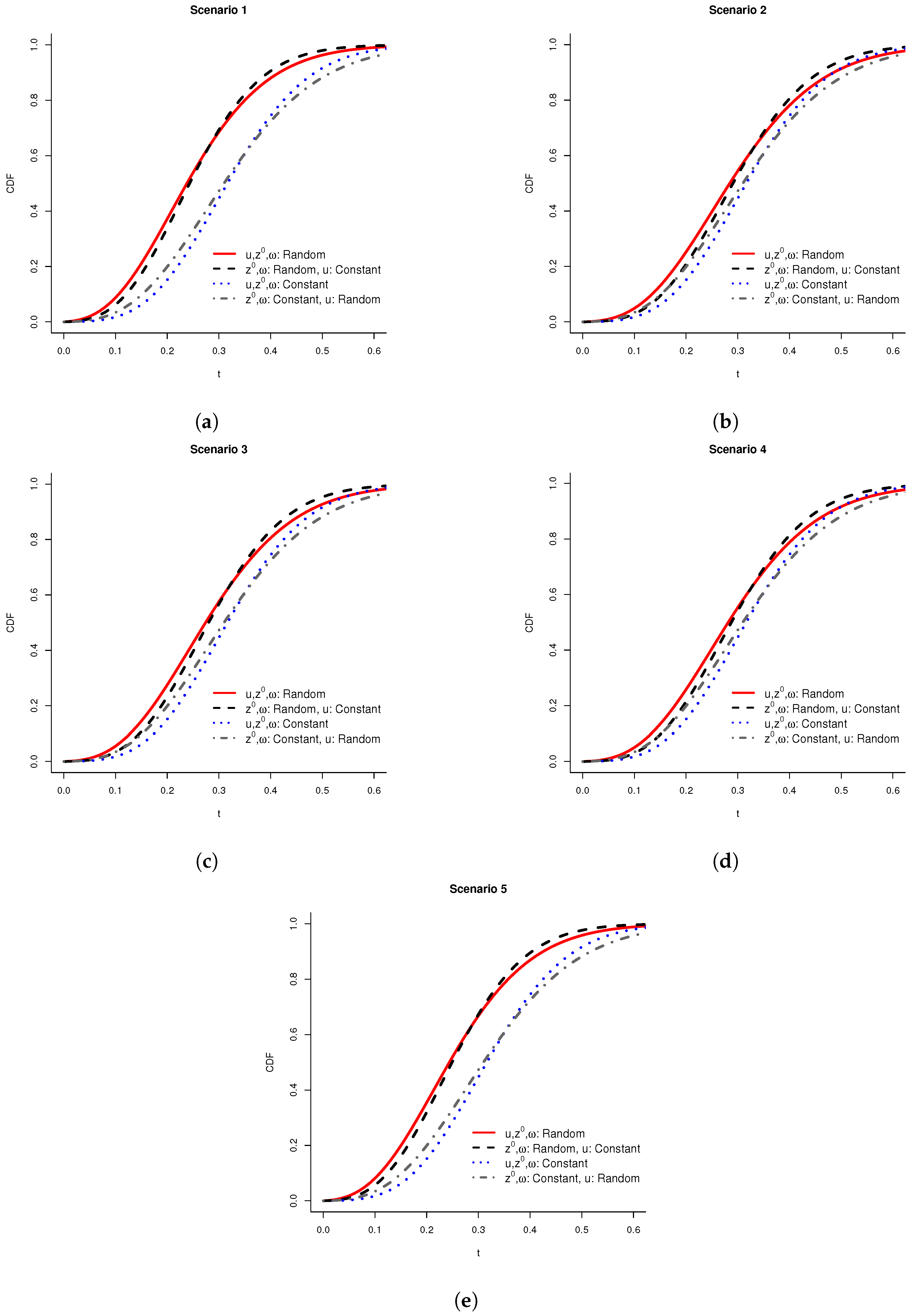
Section 4. In
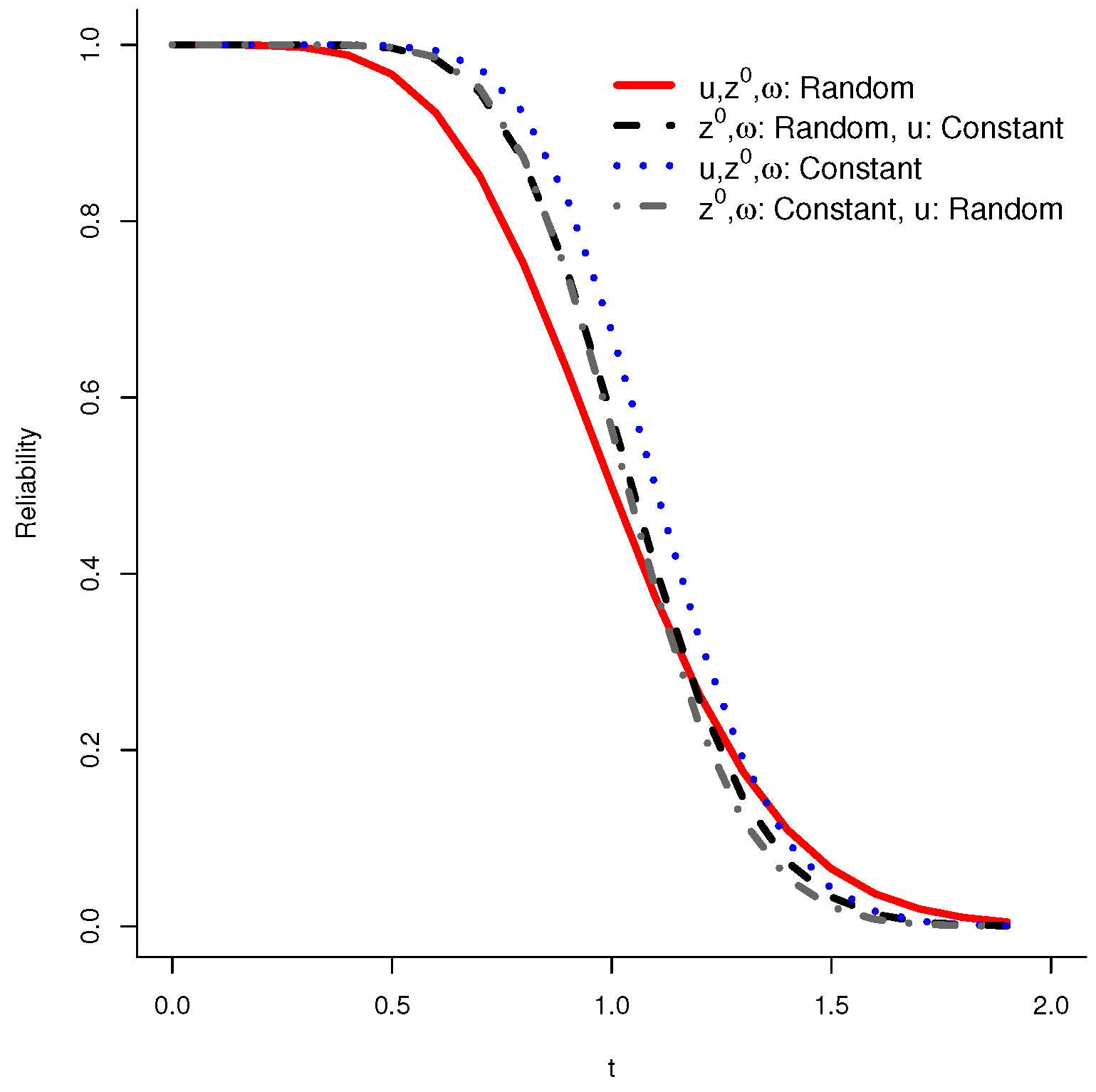
Figure 3, the obtained first-passage time CDFs via numerical integration are presented. Note that the red line in all scenarios represent the first-passage time CDF for the gamma process with three sources of variability.
For comparison purposes, we considered three additional models that have different sources of variability. Specifically, for the second model we considered the first-passage time CDF of the simple gamma process with no variability source, which in all the scenarios from
Figure 3 is represented by the dotted blue line (
) and can be obtained from (
1), for this model it was considered that
,
, and
. The third model is the gamma process with one source of variability, i.e., random scale, which in all the scenarios from
Figure 3 is represented by the dash dotted gray line (
) and that can be obtained from (
3) considering that
and
. Finally, the fourth model considers two sources of variability, specifically in the threshold
and the initial level of degradation
, but considers that the scale
u of the gamma process is constant with
, similar to the model proposed by Rodríguez-Picón et al. [
31]. The CDF of this model can be obtained by considering the first-passage time CDF of the simple gamma process and taking into account that
is random and can be obtained via the convolution operation presented in (
4). Then, the CDF can be obtained as,
This CDF can be characterized by considering the code presented in step 3 of
Section 4, by defining
as the CDF of the simple gamma process. In
Figure 3, this CDF is presented for all the scenarios in the dashed black line (
). Furthermore, in
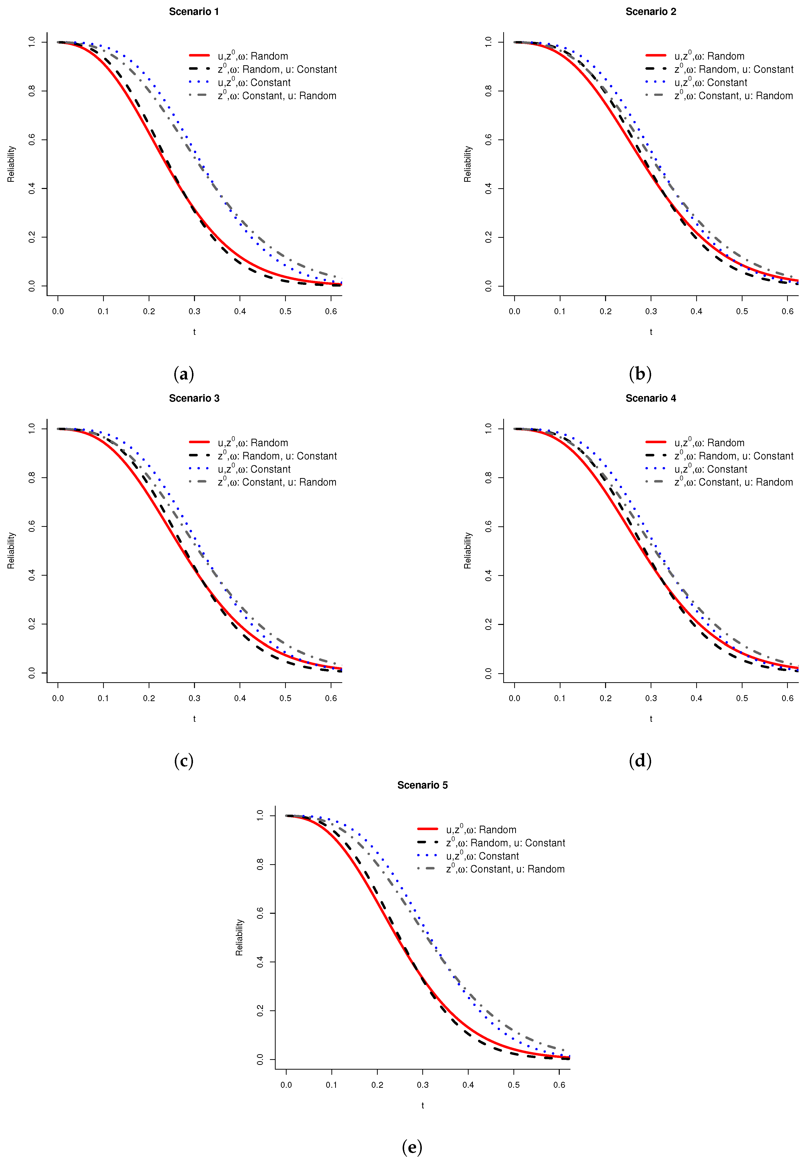
Figure 4, the estimated reliabilities are presented for the five scenarios and the four considered gamma process models with different sources of variability.
From these figures, the effect of the different sources of variability can be noted. Specifically, note that the reliability functions are different for every model in each scenario. An important aspect results by considering the first and fifth scenario from
Figure 4a,e, in these scenarios the difference between the reliabilities obtained from the models when
and
are random (reliabilities in the red continuous line and the black dashed line) is large in comparison with the other two models (dotted blue line and dash dotted gray line). It can be noted that the gamma process with three sources of variability
tends to overlap with the gamma process with two sources of variability
, indeed there is certain variation in the behavior of the reliabilities, which is due to the effect of the random scale. On the other hand, it can be noted that these two reliabilities differ from the reliabilities from the simple gamma process with no source of variability and the gamma process with random scale
, but these two reliabilities tend to overlap with certain differences due to the random scale. The difference between these two pairs of models is due to the effect of the randomness in the threshold and the initial level of degradation. Specifically, note that for the models with constant threshold and initial level it was considered that
and
which results in
, then note in
Figure 2a,e that, for the first and fifth scenarios, the distribution of
, when
and
are random, tends to be biased to the left with an approximate mean of 1.5. Furthermore, a value of 2 has a low probability of being obtained according to these distributions. Likewise, it can be noted that for scenarios 2, 3, and 4 in
Figure 4b–d the difference among the reliabilities from the models that consider randomness in
and the models that do not consider randomness in these two aspects is small. This is because, as can be noted from
Figure 2b–d, the mean of the distribution of
tends to be more close to 2 in comparison to the distributions in
Figure 2a,e.
6. Implementation in a Case Study
The case study presented by Rodríguez-Picón et al. [
31] is considered to illustrate the applicability of the proposed model, the authors discussed a degradation process based on a fatigue crack propagation dataset. Specifically, the case study consisted in the crack growth in a terminal of an electronic device, due to the characteristics of the specimen under test and the manufacturing process, the threshold
and the initial level of degradation
were random for every device. Thus, the modeling approach considered that these two characteristics were described by PDFs. Specifically, from the available data of 80 terminals, it was presented that the best fitting distribution for the threshold
was an inverse Gaussian distribution and the parameters were estimated as
. On the other hand, for the initial level of degradation
the best fitting distribution was a normal distribution with parameters estimated as
.
In this paper, a gamma process with variability in the threshold and the initial level is also considered, with the additional consideration that the scale parameter is a random variable. Thus, the proposed method described in
Section 4 is considered to analyze the degradation dataset. The first step consists in estimating the parameters of the gamma process with random scale. By considering the PDF in (
6), the fatigue crack dataset was fitted considering (
7) and the MLE method, and the parameters were estimated as
and
. Then, the distribution of
has to be characterized. As previously noted, compared with the proposed approach from Rodríguez-Picón et al. [
31], in this paper the subtraction is directly obtained via a convolution operation, instead of obtaining an approximation that then is fitted to different PDFs, which adds uncertainty to the characterization of
. The distribution
is obtained by considering the code in step 2 of
Section 4 by defining the corresponding distributions as
and
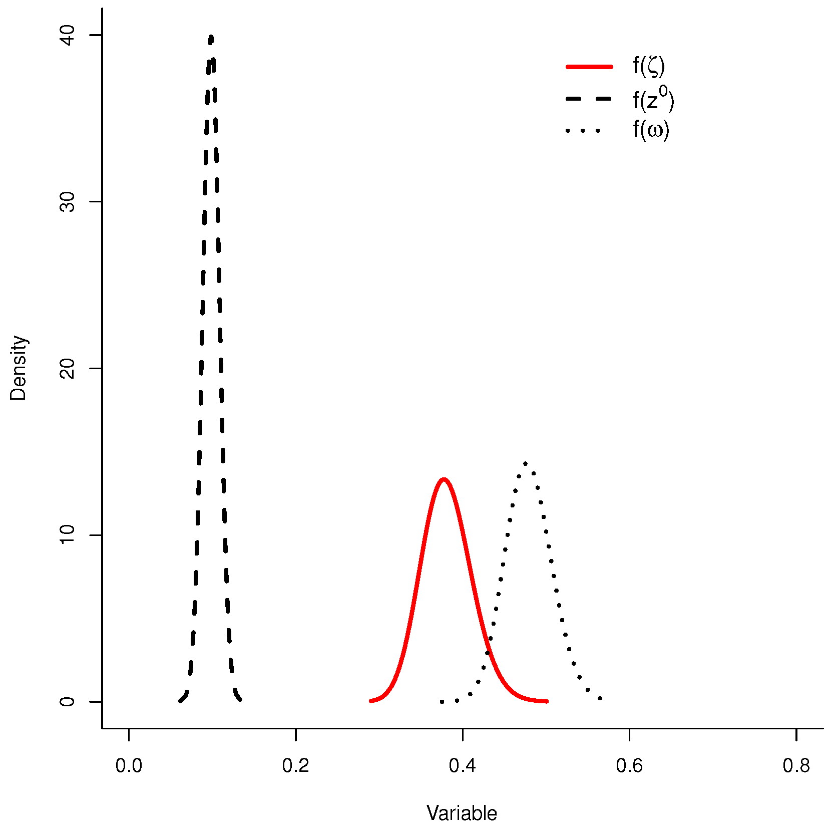
. In
Figure 5, the distributions of
,
, and
are presented. The PDF
was obtained according to the convolution operation, and denotes the effect of the subtraction
.
The PDF
along with the estimated parameters
are now used in the integral presented in (
5), which is solved with the code presented in step 3 of
Section 4. In
Figure 6, the estimated reliability functions of the gamma process with different sources of variability are presented. Specifically, the red function was obtained for the gamma process with three sources, the dashed line represents the gamma process with two sources, the gray dash dotted line represents the gamma process with one source, and the blue dotted line represents the simple gamma process with no source of variability. The effect of the sources of variability can be noted in the behavior differences of all models. Specifically, the model without sources of variability tends to overestimate the reliability in comparison with the rest of the models. On the other hand, from
to
approximately, the estimated reliability for the proposed model with three sources of variability is lowered compared with the rest of the models. Moreover, for
the reliability tends to be greater. This is due to the effect of the random scale parameter that is considered in the proposed approach.
Furthermore, the respective MTTFs for all the models were obtained based on (
8). For the proposed model with three sources of variability, the MTTF resulted in 10.66; for the model with two sources of variability, the MTTF resulted in 11.04; while for the model with one source of variability and the simple gamma process, the MTTF was obtained as 10.92 and 11.56, respectively. The effect of the sources of variability can also be noted on these estimations, as the MTTF for the model with three sources of variability is less than all the models with less sources of variability, which confirm the observations from the reliability functions.
In this paper, the gamma process without sources of variability and the gamma process with one source of variability are considered in the aims of illustrate the effect on the reliability estimation by considering inappropriate models. Specifically, these two models are inappropriate because they consider that both the initial level of degradation and the threshold are constants. In the case study, both characteristics are not constant as the initial crack length for every terminal is different, which denotes the need to consider it as random. On the other hand, the threshold is defined as the length at which the crack propagates to cause a total rupture of the terminal. This critical length is related to the width of the terminal, as each terminal has variations of their widths’ length, then the threshold must be considered as random. Thus, randomness in both the initial level and the threshold are inherent characteristics that must be considered in the modeling. On the other hand, the difference between the gamma process with two and three sources of variability relies in defining the scale parameter as random. Then, a significance test can be carried out to determine the need to define this third source of variability. The hypotheses are
is constant against
is random. The significance test considers the log-likelihood functions of the gamma process with random scale presented in (
7) and the log-likelihood function of the simple gamma process, which is defined as,
The statistical test is defined as
, where
and
are the MLE estimates. The rejection region is defined as
[
18], where
is the significance level and
. For the crack propagation data of the case study, it was obtained that
and
. Thus,
with a
, by considering a significance level of
, then
is rejected and it is concluded that the third source of variability must be considered in the model. Based on this, the model with three sources of variability is the most appropriate to describe the degradation process of the crack propagation in the case study.
7. Conclusions
In this paper, a gamma process model with three sources of variation is proposed. Specifically, it is considered that the initial level of degradation, the threshold, and the scale parameter of the gamma process are random variables that affect the degradation process. The modeling approach consists in considering the gamma model with random scale and that the difference between the initial level and the threshold is obtained through a convolution operation to obtain a distribution of the subtraction. Then, the first passage time CDF of the model is obtained by integrating out the subtraction distribution from the random scale gamma model. As this integral results in a complex form, it is numerically solved with the R software. Furthermore, the convolution operation is also solved with the R software. The codes for the solution of the integrals are provided in the manuscript to solve any combination of PDFs that can be encountered in real life case studies. From the simulation study, it was observed that, from the estimated reliabilities, the effect of random initial level, the random threshold, and the random scale can be noted as the reliability for the three sources of variation models tends to separate from the models that consider that this characteristics are constant. If the initial level and the threshold are random, but the mean of the distribution for the subtraction is close to the value of the difference when both are constant, then the reliability functions tend to have a similar behavior with slight differences. This can be noted in
Figure 4b. On the other hand, the effect of the randomness in the scale parameter can be noted in all models that considered this condition in comparison with the models with constant scale. This can be clearly noted in
Figure 4a.
From the case study, it was observed that there are clear differences in the estimated reliability function from the proposed model with three sources of variation and the model with two sources. As a result of the random scale parameter, the reliability tends to be lower from to and greater for . The proposed approach can be considered for case studies where the degradation process has several conditions that affect the degradation process, which can be determined as random effects. The proposed approach can be extended for future research considering more sources of variability; for example, a modification of the structure of the gamma process can be considered to make that both the scale and shape parameter of the model are random variables. Furthermore, measurement errors may be considered in the modeling approach, as this is an inherent source of variation that can be found in most of the degradation process. These extensions present important challenges to develop a comprehensive approach; apart from establishing further sources of variability, the significance of these sources should be studied to determine how appropriate such sources can be in order to define a degradation model. Furthermore, the inherent characteristics of the particular case study should drive the consideration of a specific set of sources of variability. As in the case study in this paper, the inherent characteristics of the device define the need to consider randomness in the initial level and the threshold, while the variability in the scale parameter was determined according to a significance test. On the other hand, the characteristics of the experimental design that is considered to perform a degradation test may determine the need to consider block effects as another source of variability. Specific efforts should be made to test the proposition that there is independent variation in the parameters variation of multiple sources.

 ,
, 


