
Modern Dimensional Analysis-Based Steel Column Heat Transfer Evaluation Using Multiple Experiments

 ,
,  ,
,
Abstract
:1. Introduction
- MDA does not require deep knowledge in the field, only the review of the variables (along with their dimensions), which can, to a certain extent, influence the analyzed phenomenon;
- the unitary protocol of the MDA allows the automatic elimination of variables with insignificant/irrelevant influence (either from the physical point of view or from the magnitude point of view), without the researcher having any other algorithm to apply;
- MDA provides, in all cases, the complete set of dimensionless variables and therefore of the ML, which the rest of the methods cannot provide, except in very special cases;
- from this complete set, by eliminating some variables, which are identical to the prototype and the model, one can formulate/obtain the particular sets related to simpler cases.
2. Materials and Models
- Version I, where the set of independent variables was , was chosen:
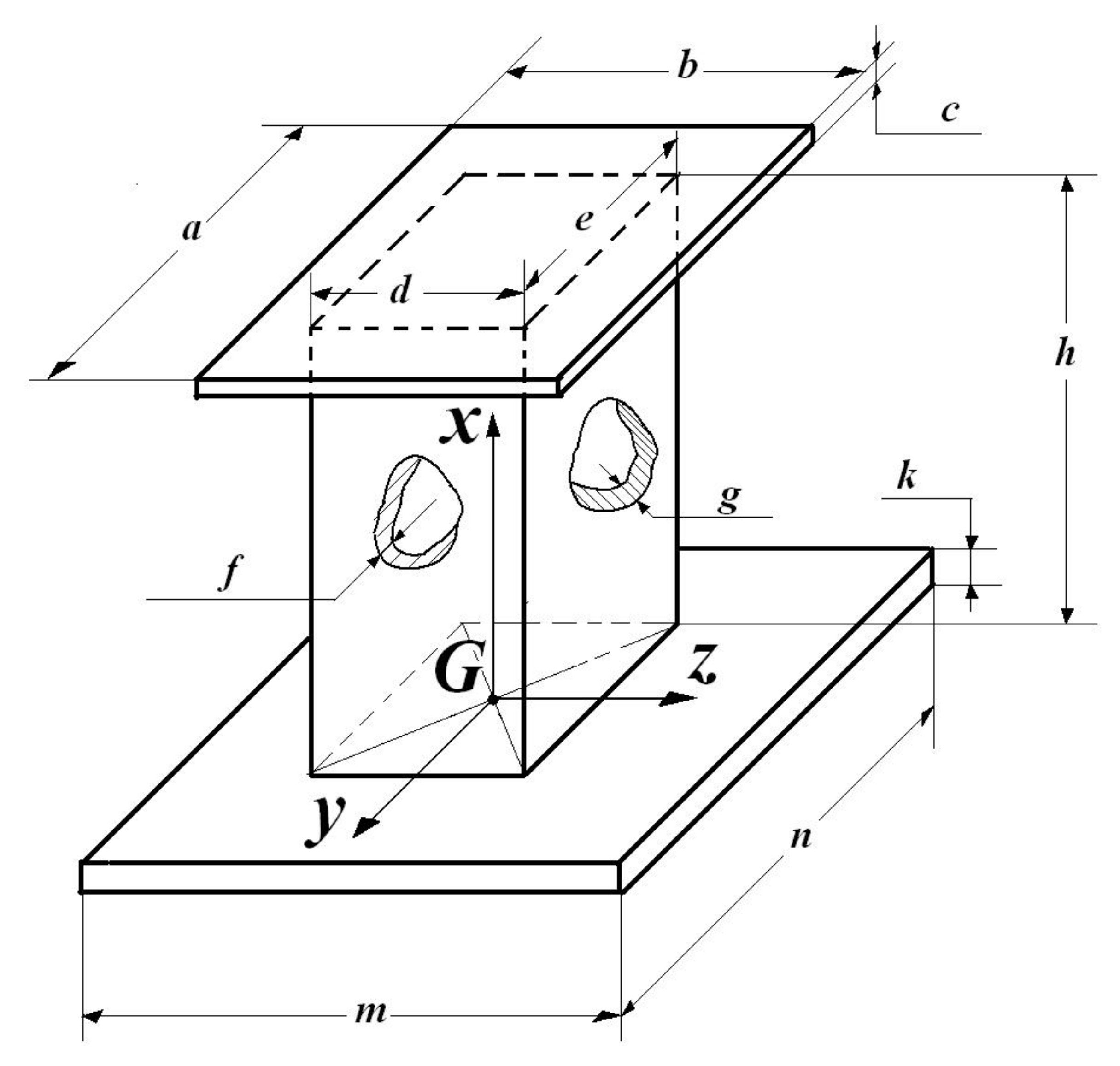
- Version II, where the set of independent variables was , was chosen:where: represents the invested heat; —the heat rate; —the beam dimension along direction z; —the temperature variation; —the time; —the thermal conductivity; —the shape factor; —the perimeter of the cross-section; —the area of the cross-section; —the scale factor of the variable , with index “1” for prototype, respectively with “2” for the model.
- The case of the quadratic section represents a particular case of the rectangular one, where on the two directions y and z there exist the same dimensions and the same scale factors;
- If it is desired, however, that the scale factors of the dimensions along the z and y directions have different values, respectively, one should admit different thicknesses in the two directions, and then one will have and correspondingly these elements/variables for the model will be rigorously obtained only from the ML;
- Taking into account that length is considered an independent variable, and thus freely chosen a priori, for both the prototype and model, the Model Law elements for the rest of the dimensions can be ignored, each having the same scale factor of lengths , which is why it makes no sense to analyze them and their validity;
- The advantage of including the shape factor in the set of independent variables, in addition to that of the length , resides in the fact that one will be free of the restriction of a geometric similarity of the cross-sections of the prototype and the model (so, let us have, for example, only rectangular sections), allowing one to accept a section of another shape in the model, only to respect the initially established scale factor.
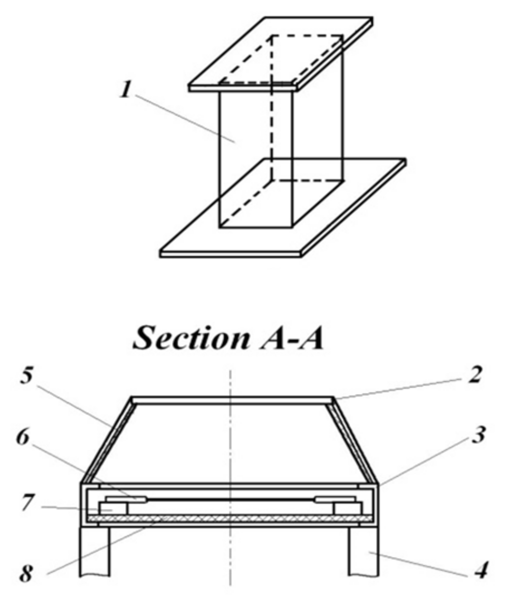
- mounting the stand, with the provision of rigorous thermal insulation with the help of suitable special mattresses (Figure 3);
- mounting, on the lower plate with the dimensions of the tested structural element, a thermocouple type K (intended to control the nominal temperature ), as well as all thermoresistances type PT 100-402 at the elevation level , according to Table 2;
- connecting the thermoresistances to the data acquisition system;
- checking the proper functioning of all elements;
- selection of nominal temperature ;
- selection of the steps of the heating regime;
- connecting the stand to the 380 V power source;
- starting the installation and monitoring the reaching of the temperature ;
- recording the electrical energy consumed , as well as the time required to reach this stabilized thermal regime;
- resumption of stages to reach all nominal temperatures of .
- The control electronic temperature system also has a self-learning function; so, basically, after the first cycle of reaching the nominal temperature , it will ensure the temperature control within very limited limits. For example, at , the thermal oscillations related to the regulation were at maximum ;
- The achievement of a stabilized temperature regime was considered to be achieved; when at the level of the last thermoresistance PT 100-402 (near the upper part of the tested structural element) the maximum temperature oscillations were observed for a period of minimum
- —temperature difference reached during heating;
- —the time required to reach it;
- —the unfolded areas of the k heat-insulating blankets applied around the stand, having the thickness .
- in relation (5), for each interval , the corresponding temperature difference ( ) will be considered and applied to the time intervals corresponding to ;
- the temperature differences are determined with relation (6) individually for each interval before, considering the average temperature related to each interval, respectively;
- the term , being constant, will multiply the sum of the partial products related to these intervals.
3. Results and Discussions
- Prototype (structural element made at 1:1 scale) model (structural element made at 1:2 scale), symbolized by (1:2/1:1) Model/Prototype;
- Prototype (structural element made at 1:2 scale) model (structural element made at 1:4 scale), symbolized by (1:4/1:2) Model/Prototype;
- Prototype (structural element made at 1:1 scale) model (structural element made at 1:4 scale), symbolized by (1:4/1:1) Model/Prototype;
- Prototype (structural element made at 1:1 scale) model (structural element made at 1:10 scale), symbolized by (1:2/1:10) Model/Prototype;
- Prototype (structural element made at 1:2 scale) model (structural element made at 1:10 scale), symbolized by (1:4/1:10) Model/Prototype;
- Prototype (structural element made at 1:1 scale) model (structural element made at 1:10 scale), symbolized by (1:4/1:10) Model/Prototype;

| Measured Values | |||||
|---|---|---|---|---|---|
| Model/prototype | Tmin–Tmax | ||||
| 23–100 | 2 | 0.677419 | 0.98208 | 0.979727 | |
| 100–200 | 2 | 0.37037 | 2.186656 | 2.281555 | |
| 1:2/1.0 | 200–300 | 2 | 0.576923 | 0.579094 | 0.549528 |
| 300–400 | 2 | 1.05 | 0.404082 | 0.356384 | |
| 400–450 | 2 | 0.769231 | 0.610836 | 0.558164 | |
| 450–500 | 2 | 0.777778 | 0.525086 | 0.462721 | |
| 23–100 | 2 | 1.809524 | 0.352042 | 0.333138 | |
| 100–200 | 2 | 0.55 | 0.987704 | 0.982251 | |
| 200–300 | 2 | 3.333333 | 0.459803 | 0.370959 | |
| 1:4/1:2 | 300–400 | 2 | 1.428571 | 0.693323 | 0.599302 |
| 400–450 | 2 | 6 | 0.517304 | 0.381264 | |
| 450–500 | 2 | 0.785714 | 0.678703 | 0.572806 | |
| 23–100 | 4 | 1.225806 | 0.345734 | 0.326384 | |
| 100–200 | 4 | 0.203704 | 2.159769 | 2.24106 | |
| 1:4/1.0 | 200–300 | 4 | 1.923077 | 0.26627 | 0.203852 |
| 300–400 | 4 | 1.5 | 0.280159 | 0.213582 | |
| 400–450 | 4 | 4.615385 | 0.315988 | 0.212808 | |
| 450–500 | 4 | 0.611111 | 0.356377 | 0.265049 | |
| 23–100 | 10.71479 | 1.080645 | 0.516392 | 0.519029 | |
| 100–200 | 10.71479 | 0.430556 | 1.480349 | 1.703182 | |
| 1:10/1.0 | 200–300 | 10.71479 | 2.092308 | 0.304194 | 0.32068 |
| 300–400 | 10.71479 | 1.605 | 0.490396 | 0.519326 | |
| 400–450 | 10.71479 | 1.7 | 0.317508 | 0.348966 | |
| 450–500 | 10.71479 | 0.638889 | 0.313694 | 0.345774 | |
| 23–100 | 5.357394 | 1.595238 | 0.525814 | 0.529769 | |
| 100–200 | 5.357394 | 1.1625 | 0.676992 | 0.7465 | |
| 1:10/1:2 | 200–300 | 5.357394 | 3.626667 | 0.525292 | 0.583555 |
| 300–400 | 5.357394 | 1.528571 | 1.213605 | 1.457208 | |
| 400–450 | 5.357394 | 2.21 | 0.519793 | 0.625203 | |
| 450–500 | 5.357394 | 0.821429 | 0.597414 | 0.747262 | |
| 23–100 | 2.678697 | 0.881579 | 1.493611 | 1.590241 | |
| 100–200 | 2.678697 | 2.113636 | 0.68542 | 0.759989 | |
| 1:10/1:4 | 200–300 | 2.678697 | 1.088 | 1.142427 | 1.573096 |
| 300–400 | 2.678697 | 1.07 | 1.750417 | 2.431507 | |
| 400–450 | 2.678697 | 0.368333 | 1.004811 | 1.639818 | |
| 450–500 | 2.678697 | 1.045455 | 0.880229 | 1.304563 | |
| Reference Values (Values for Validation) | Calculated Values with the Model Law | |||||
|---|---|---|---|---|---|---|
| Model/Prototype | ||||||
| 0.25 | 0.66528 | 0.663686 | 0.66528 | 0.663686 | 0.25 | |
| 0.25 | 0.809873 | 0.84502 | 0.809873 | 0.84502 | 0.25 | |
| 1:2/1.0 | 0.25 | 0.334093 | 0.317035 | 0.334093 | 0.317035 | 0.25 |
| 0.25 | 0.424286 | 0.374203 | 0.424286 | 0.374203 | 0.25 | |
| 0.25 | 0.469873 | 0.429357 | 0.469873 | 0.429357 | 0.25 | |
| 0.25 | 0.4084 | 0.359894 | 0.4084 | 0.359894 | 0.25 | |
| 0.25 | 0.636907 | 1.449594 | 0.637029 | 0.602821 | 0.25 | |
| 0.25 | 0.543237 | 0.540238 | 0.543237 | 0.540238 | 0.25 | |
| 0.25 | 1.532678 | 1.236531 | 1.532678 | 1.236531 | 0.25 | |
| 1:4/1:2 | 0.25 | 0.990462 | 0.856146 | 0.990462 | 0.856146 | 0.25 |
| 0.25 | 3.103827 | 2.287582 | 3.103827 | 2.287582 | 0.25 | |
| 0.25 | 0.533267 | 0.450062 | 0.533267 | 0.450062 | 0.25 | |
| 0.0625 | 0.423721 | 0.400084 | 0.423803 | 0.400084 | 0.0625 | |
| 0.0625 | 0.439953 | 0.456512 | 0.439953 | 0.456512 | 0.0625 | |
| 1:4/1.0 | 0.0625 | 0.512057 | 0.392024 | 0.512057 | 0.392024 | 0.0625 |
| 0.0625 | 0.420239 | 0.320373 | 0.420239 | 0.320373 | 0.0625 | |
| 0.0625 | 1.458406 | 0.982188 | 1.458406 | 0.982188 | 0.0625 | |
| 0.0625 | 0.533267 | 0.161975 | 0.217786 | 0.161975 | 0.0625 | |
| 0.008 | 0.558036 | 0.560886 | 0.558036 | 0.560886 | 0.008 | |
| 0.008 | 0.637373 | 0.733314 | 0.637373 | 0.733314 | 0.008 | |
| 1:10/1.0 | 0.008 | 0.636467 | 0.67096 | 0.636467 | 0.67096 | 0.008 |
| 0.008 | 0.787085 | 0.833518 | 0.787085 | 0.833518 | 0.008 | |
| 0.008 | 0.539764 | 0.593241 | 0.539764 | 0.593241 | 0.008 | |
| 0.008 | 0.200415 | 0.220911 | 0.200415 | 0.220911 | 0.008 | |
| 0.031999 | 0.838799 | 0.845108 | 0.838799 | 0.845108 | 0.031998 | |
| 0.031999 | 0.787004 | 0.867807 | 0.787004 | 0.867807 | 0.031999 | |
| 1:10/1:2 | 0.031999 | 1.905058 | 2.116358 | 1.905058 | 2.116358 | 0.031999 |
| 0.031999 | 1.855082 | 2.227447 | 1.855082 | 2.227447 | 0.031999 | |
| 0.031999 | 1.148743 | 1.381698 | 1.148743 | 1.381698 | 0.031999 | |
| 0.031999 | 0.490733 | 0.613822 | 0.490733 | 0.613822 | 0.031999 | |
| 0.127994 | 1.316736 | 1.401923 | 1.316736 | 1.401923 | 0.127994 | |
| 0.127994 | 1.448729 | 1.606341 | 1.448729 | 1.606341 | 0.127994 | |
| 1:10/1:4 | 0.127994 | 1.24296 | 1.711529 | 1.24296 | 1.711529 | 0.127994 |
| 0.127994 | 1.872946 | 2.601712 | 1.872946 | 2.601712 | 0.127994 | |
| 0.127994 | 0.370105 | 0.604 | 0.370105 | 0.604 | 0.127994 | |
| 0.127994 | 0.920239 | 1.363862 | 0.920239 | 1.363862 | 0.127994 | |
4. Final Remarks
- With the data obtained in reference [40], for the two significant versions I and II, the validation calculations of the significant elements of the ML were performed;
- MDA presented a series of facilities, regarding its simplification, and were deduced for the general case and analyzed in detail in the Introduction section;
- In this sense, it is also worth highlighting those related to ignoring some scale factors in the event of:
- existing implicit correlations (for example: the same type of material existing in the prototype and in the model, or there being identical environmental and deployment conditions for the experimental investigations in the prototype and in the model);
- existing over-definition of the parameters (such as, for example, accepting the same scale of all lengths when the scales and scale factors of the areas no longer have a purpose, so they can be neglected from the above-mentioned analysis);
- With the help of the variables (,), it became possible to design models even with different wall thicknesses along the two coordinates , i.e., to ensure models with different areas, obviously; with strict compliance to the scales of these variables imposed by the related elements of the ML, the obligation of the existence of a geometric similarity of the cross-sections (prototype-model) can be eliminated;
- The case of the quadratic section was an obvious particular case of the rectangular one;
- The advantage of the simultaneous inclusion of both length () and shape factor in the set of independent variables ensured the definition of more general models; where the preservation of geometric similarity is not mandatory, the model can also have a different cross-sectional shape, only to provide a certain scale factor for ;
- Inclusion of among the elements of the A matrix also provides us with the opportunity (if needed) to choose another material for the model in order to reduce the cost price of making and/or testing the model;
- Considering or as independent variables also ensures a great freedom in choosing the thermal-stress strategy of the model compared with that of the prototype;
- Inclusion of in the set of independent variables provides the researcher the opportunity to choose a thermal regime as favorable as possible for loading the model in relation to the prototype;
- Considering the time of exposure to a certain thermal regime in the set of independent variables provides another benefit of the use/application of MDA to follow the thermal transfer to structures subject to fires.
5. Conclusions
Author Contributions
Funding
Institutional Review Board Statement
Informed Consent Statement
Data Availability Statement
Conflicts of Interest
References
- Munteanu (Száva), I.R. Investigation Concerning Temperature Field Propagation along Reduced Scale Modelled Metal Structures. Ph.D. Thesis, Transilvania University of Brasov, Brașov, Romania, 2018. [Google Scholar]
- Al-Homoud, M.S. Performance characteristics and practical applications of common building thermal insulation materials. Build. Environ. 2005, 40, 353–366. [Google Scholar] [CrossRef]
- Bailey, C. Indicative fire tests to investigate the behaviour of cellular beams protected with intumescent coatings. Fire Saf. J. 2004, 39, 689–709. [Google Scholar] [CrossRef]
- Khan, M.A.; Irfan, S.; Rizvi, Z.; Ahmad, J. A numerical study on the validation of thermal formulations towards the behaviour of RC beams. Mater. Today Proc. 2019, 17, 227–234. [Google Scholar] [CrossRef]
- Lawson, R. Fire engineering design of steel and composite buildings. J. Constr. Steel Res. 2001, 57, 1233–1247. [Google Scholar] [CrossRef]
- Noack, J.; Rolfes, R.; Tessmer, J. New layerwise theories and finite elements for efficient thermal analysis of hybrid structures. Comput. Struct. 2003, 81, 2525–2538. [Google Scholar] [CrossRef]
- Papadopoulos, A. State of the art in thermal insulation materials and aims for future developments. Energy Build. 2005, 37, 77–86. [Google Scholar] [CrossRef]
- Quintier, G.J. Fundamentals of Fire Phenomena; John Willey & Sons: Hoboken, NJ, USA, 2006. [Google Scholar]
- Tafreshi, A.; Marzo, M. Foams and gels as fire protection agents. Fire Saf. J. 1999, 33, 295–305. [Google Scholar] [CrossRef]
- Wong, M.; Ghojel, J. Sensitivity analysis of heat transfer formulations for insulated structural steel components. Fire Saf. J. 2003, 38, 187–201. [Google Scholar] [CrossRef]
- Yang, K.-C.; Chen, S.-J.; Lin, C.-C.; Lee, H.-H. Experimental study on local buckling of fire-resisting steel columns under fire load. J. Constr. Steel Res. 2005, 61, 553–565. [Google Scholar] [CrossRef]
- Guo, Z.; Wang, Y.; Lu, N.; Zhang, H.; Zhu, F. Behaviour of a two-pinned steel arch at elevated temperatures. Thin-Walled Struct. 2016, 107, 248–256. [Google Scholar] [CrossRef]
- Choe, L.; Zhang, C.; Luecke, W.E.; Gross, J.L.; Varma, A.H. Influence of Material Models on Predicting the Fire Behavior of Steel Columns. Fire Technol. 2016, 53, 375–400. [Google Scholar] [CrossRef]
- Ahn, H.J.; An, J.H.; Yeo, I.H.; Hwang, K.J. The relationship between temperature behaviors and section factors of fire spray protection coated composite beams exposed to standard fire. Int. J. Steel Struct. 2015, 15, 853–861. [Google Scholar] [CrossRef]
- Zhang, C.; Silva, J.G.; Weinschenk, C.G.; Kamikawa, D.; Hasemi, Y. Simulation Methodology for Coupled Fire-Structure Analysis: Modeling Localized Fire Tests on a Steel Column. Fire Technol. 2016, 52, 239–262. [Google Scholar] [CrossRef]
- Bączkiewicz, J.; Malaska, M.; Pajunen, S.; Heinisuo, M. Experimental and numerical study on temperature distribution of square hollow section joints. J. Constr. Steel Res. 2018, 142, 31–43. [Google Scholar] [CrossRef]
- He, S.-B.; Shao, Y.-B.; Zhang, H.-Y.; Yang, D.-P.; Long, F.-L. Experimental study on circular hollow section (CHS) tubular K-joints at elevated temperature. Eng. Fail. Anal. 2013, 34, 204–216. [Google Scholar] [CrossRef]
- He, S.; Shao, Y.; Zhang, H.; Wang, Q. Parametric study on performance of circular tubular K-joints at elevated temperature. Fire Saf. J. 2015, 71, 174–186. [Google Scholar] [CrossRef]
- He, S.; Shao, Y.; Zhang, H. Evaluation on fire resistance of tubular K-joints based on critical temperature method. J. Constr. Steel Res. 2015, 115, 398–406. [Google Scholar] [CrossRef]
- Gao, F.; Guan, X.-Q.; Zhu, H.-P.; Liu, X.-N. Fire resistance behaviour of tubular T-joints reinforced with collar plates. J. Constr. Steel Res. 2015, 115, 106–120. [Google Scholar] [CrossRef]
- Kado, B.; Mohammad, S.; Lee, Y.H.; Shek, P.N.; Kadir, M.A. Ab Temperature Analysis of Steel Hollow Column Exposed to Standard Fire. J. Struct. Technol. 2018, 3, 1–8. [Google Scholar]
- Ferraz, G.; Santiago, A.; Rodrigues, J.P.; Barata, P. Thermal Analysis of Hollow Steel Columns Exposed to Localised Fires. Fire Technol. 2016, 52, 663–681. [Google Scholar] [CrossRef]
- Franssen, J.-M. Calculation of temperature in fire-exposed bare steel structures: Comparison between ENV 1993-1-2 and EN 1993-1-2. Fire Saf. J. 2006, 41, 139–143. [Google Scholar] [CrossRef]
- Ghojel, J.; Wong, M. Heat transfer model for unprotected steel members in a standard compartment fire with participating medium. J. Constr. Steel Res. 2005, 61, 825–833. [Google Scholar] [CrossRef]
- Carabogdan, G.I.; Badea, A.; Brătianu, C.; Muşatescu, V. Methods of Analysis of Thermal Energy Processes and Systems; Technical Publishing House: Bucharest, Romania, 1989. [Google Scholar]
- Barenblatt, G.I. Dimensional Analysis; Gordon and Breach: New York, NY, USA, 1987. [Google Scholar]
- Carlson, D.E. Some New Results in Dimensional Analysis. Arch. Ration. Mech. Anal. 1978, 68, 191–210. [Google Scholar] [CrossRef]
- Chen, W.-K. Algebraic theory of dimensional analysis. J. Frankl. Inst. 1971, 292, 403–422. [Google Scholar] [CrossRef]
- Coyle, R.G.; Ballico-Lay, B. Concepts and software for dimensional analysis in modeling. IEEE Trans. Syst. Man, Cybern. 1984, SMC-14, 478–482. [Google Scholar] [CrossRef]
- Gibbings, J.C. Dimensional Analysis. J. Phys. A-Math. Gen. 1980, 13, 75–89. [Google Scholar] [CrossRef]
- Martins, R.D.A. The origin of dimensional analysis. J. Frankl. Inst. 1981, 311, 331–337. [Google Scholar] [CrossRef]
- El Nakla, M. On fluid-to-fluid modeling of film boiling heat transfer using dimensional analysis. Int. J. Multiph. Flow 2011, 37, 229–234. [Google Scholar] [CrossRef]
- Nezhad, A.H.; Shamsoddini, R. Numerical three-dimensional analysis of the mechanism of flow and heat transfer in a vortex tube. Therm. Sci. 2009, 13, 183–196. [Google Scholar] [CrossRef]
- Pankhurst, R.C. Dimensional Analysis and Scale Factor; Chapman & Hall Ltd.: London, UK, 1964. [Google Scholar]
- Remillard, W.J. Applying dimensional analysis. Am. J. Phys. 1983, 51, 137–140. [Google Scholar] [CrossRef]
- Romberg, G. Beitrag zur Dimensionsanalyse. Ingenieur-Archiv 1985, 55, 401–412. [Google Scholar] [CrossRef]
- Schnittger, J.R. Dimensional Analysis in Design. J. Vib. Acoust. 1988, 110, 401–407. [Google Scholar] [CrossRef]
- Szekeres, P. The mathematical foundations of dimensional analysis and the question of fundamental units. Int. J. Theor. Phys. 1978, 17, 957–974. [Google Scholar] [CrossRef]
- Száva, I.R.; Șova, D.; Dani, P.; Élesztős, P.; Száva, I.; Vlase, S. Experimental Validation of Model Heat Transfer in Rectangular Hole Beams Using Modern Dimensional Analysis. Mathematics 2022, 10, 409. [Google Scholar] [CrossRef]
- Sova, D.; Száva, I.R.; Jármai, K.; Száva, I.; Vlase, S. Heat transfer analysis in a beam with rectangular-hole using Modern Dimensional Analysis. Mathematics 2022, 10, 409. [Google Scholar]
- Szirtes, T. The Fine Art of Modelling. SPAR J. Eng. Technol. 1992, 1, 37. [Google Scholar]
- Szirtes, T. Applied Dimensional Analysis and Modelling; McGraw-Hill: Toronto, ON, Canada, 1998. [Google Scholar]
- Száva, I.; Szirtes, T.; Dani, P. An Application of Dimensional Model Theory in The Determination of the Deformation of a Structure. Eng. Mech. 2006, 13, 31–39. [Google Scholar]
- Dani, P.; Száva, I.R.; Kiss, I.; Száva, I.; Popa, G. Principle schema of an original full-, and reduced-scale testing bench, destined to fire protection investigations. Ann. Fac. Eng. Hunedoara-Int. J. Eng. 2018, 16, 149–152. [Google Scholar]
- Turzó, G.; Száva, I.R.; Gálfi, B.-P.; Száva, I.; Vlase, S.; Hoța, H. Temperature distribution of the straight bar, fixed into a heated plane surface. Fire Mater. 2018, 42, 202–212. [Google Scholar] [CrossRef]
- Trif, I.; Asztalos, Z.; Kiss, I.; Élesztős, P.; Száva, I.; Popa, G. Implementation of the Modern Dimensional Analysis in Engineering Problems; Basic Theoretical Layouts. Ann. Fac. Eng. Hunedoara 2019, 17, 73–76. [Google Scholar]


| Dimensions, in m for Element at Scale | ||||
|---|---|---|---|---|
| 1:1 | 1:2 | 1:4 | 1:10 | |
| a | 0.370 | 0.185 | 0.108 | 0.0370 |
| b | 0.370 | 0.185 | 0.108 | 0.0370 |
| c | 0.006 | 0.003 | 0.0015 | 0.0015 |
| d | 0.350 | 0.175 | 0.0875 | 0.0030 |
| e | 0.350 | 0.175 | 0.0875 | 0.0030 |
| f | 0.016 | 0.008 | 0.004 | 0.0015 |
| g | 0.016 | 0.008 | 0.004 | 0.0015 |
| h | 0.400 | 0.200 | 0.100 | 0.400 |
| k | 0.010 | 0.005 | 0.0025 | 0.0015 |
| m | 0.450 | 0.450 | 0.450 | 0.450 |
| n | 0.450 | 0.450 | 0.450 | 0.450 |
| At Scale 1:1 | At Scale 1:2 | At Scale 1:4 | At Scale 1:10 |
|---|---|---|---|
| 0.020 | 0.020 | 0.020 | 0.015 |
| 0.110 | 0.060 | 0.055 | 0.030 |
| 0.200 | 0.105 | 0.090 | 0.045 |
| 0.290 | 0.150 | 0.060 | |
| 0.380 | 0.190 | 0.100 | |
| 0.200 | |||
| 0.400 | |||
| 0.460 | |||
| 0.495 |
| Structural Element | ||||||||
|---|---|---|---|---|---|---|---|---|
| At scale 1:10 | 23–100 | 0.7017543 | 0.5 | 1,800,000 | 77 | 20.34095 | 15,231.3 | 1,784,769 |
| 100–200 | 0.7017543 | 0.8 | 2,880,000 | 100 | 20.34095 | 19,155.56 | 2,860,844 | |
| 200–300 | 0.7017543 | 1.4 | 5,040,000 | 100 | 20.34095 | 19,155.56 | 5,020,844 | |
| 300–400 | 0.7017543 | 2.1 | 7,560,000 | 100 | 20.34095 | 28,088.82 | 7,531,911 | |
| 400–450 | 0.7017543 | 0.8 | 2,880,000 | 50 | 20.34095 | 18,910.72 | 2,861,089 | |
| 450–500 | 0.7017543 | 0.5 | 1,800,000 | 50 | 20.34095 | 7799.208 | 1,792,201 | |
| At scale 1:4 | 23–100 | 0.2619760 | 0.4 | 1,440,000 | 77 | 20.07323 | 84,810.39 | 1,355,189.6 |
| 100–200 | 0.2619760 | 0.6 | 2,160,000 | 100 | 20.07323 | 185,272.3 | 1,974,727.7 | |
| 200–300 | 0.2619760 | 1.4 | 5,040,000 | 100 | 20.07323 | 1,000,576 | 4,039,424 | |
| 300–400 | 0.2619760 | 1.4 | 5,040,000 | 100 | 20.07323 | 1,018,576 | 4,021,424.3 | |
| 400–450 | 0.2619760 | 2.9 | 1,0440,000 | 50 | 20.07323 | 2,709,526 | 7,730,474.3 | |
| 450–500 | 0.2619760 | 0.7 | 2,520,000 | 50 | 20.07323 | 572,461.5 | 1,947,538.5 | |
| At scale 1:2 | 23–100 | 0.1309880 | 0.6 | 2,160,000 | 77 | 19.17165 | 32,233.53 | 2,127,766.5 |
| 100–200 | 0.1309880 | 1.1 | 3,960,000 | 100 | 19.17165 | 324,889.8 | 3,635,110.2 | |
| 200–300 | 0.1309880 | 0.8 | 2,880,000 | 100 | 19.17165 | 244,466.6 | 2,635,533.4 | |
| 300–400 | 0.1309880 | 1.3 | 4,680,000 | 100 | 19.17165 | 619,849.7 | 4,060,150.3 | |
| 400–450 | 0.1309880 | 0.8 | 2,880,000 | 50 | 19.17165 | 389,373 | 2,490,627 | |
| 450–500 | 0.1309880 | 1.2 | 4,320,000 | 50 | 19.17165 | 667,908.9 | 3,652,091.1 | |
| At scale 1:1 | 23–100 | 0.0654940 | 0.9 | 3,240,000 | 77 | 15.55354 | 41,696.8 | 3,198,303.2 |
| 100–200 | 0.0654940 | 1.4 | 5,040,000 | 100 | 15.55354 | 323,210 | 4,716,790 | |
| 200–300 | 0.0654940 | 2.3 | 8,280,000 | 100 | 15.55354 | 391,377.5 | 7,888,622.5 | |
| 300–400 | 0.0654940 | 2.8 | 10,080,000 | 100 | 15.55354 | 510,624.9 | 9,569,375.1 | |
| 400–450 | 0.0654940 | 1.6 | 5,760,000 | 50 | 15.55354 | 459,366.7 | 5,300,633.3 | |
| 450–500 | 0.0654940 | 2.7 | 9,720,000 | 50 | 15.55354 | 777,565.4 | 8,942,434.6 |
| Structural Element | |||||||
|---|---|---|---|---|---|---|---|
| At scale 1:10 | 23–100 | 849,960 | 834,728.7 | 2010 | 7.577763 | 887.9446 | 415.2879 |
| 100–200 | 1,359,936 | 1,340,780 | 2790 | 6.865792 | 1025.392 | 480.5665 | |
| 200–300 | 2,379,888 | 2,360,732 | 3264 | 5.868738 | 1538.249 | 723.2636 | |
| 300–400 | 3,569,832 | 3,541,743 | 1926 | 14.58402 | 3910.65 | 1838.911 | |
| 400–450 | 1,359,936 | 1,341,025 | 1326 | 14.26148 | 2157.684 | 1011.331 | |
| 450–500 | 849,960 | 842,160.8 | 690 | 11.3032 | 2597.392 | 1220.523 | |
| At scale 1:4 | 23–100 | 679,968 | 595,157.6 | 2280 | 37.19754 | 594.3814 | 261.034 |
| 100–200 | 1,019,952 | 834,679.7 | 1320 | 140.3578 | 1496.006 | 632.3331 | |
| 200–300 | 2,379,888 | 1,379,312 | 3000 | 333.5253 | 1346.475 | 459.7707 | |
| 300–400 | 2,379,888 | 1,361,312 | 1800 | 565.8754 | 2234.125 | 756.2846 | |
| 400–450 | 4,929,768 | 2,220,242 | 3600 | 752.646 | 2147.354 | 616.734 | |
| 450–500 | 1,189,944 | 617,482.5 | 660 | 867.3659 | 2950.816 | 935.5796 | |
| At scale 1:2 | 23–100 | 1,019,952 | 987,718.5 | 1260 | 25.58217 | 1688.704 | 783.9035 |
| 100–200 | 1,869,912 | 1,545,022 | 2400 | 135.3708 | 1514.629 | 643.7592 | |
| 200–300 | 1,359,936 | 1,115,469 | 900 | 271.6296 | 2928.37 | 1239.41 | |
| 300–400 | 220,9896 | 1,590,046 | 1260 | 491.9442 | 3222.342 | 1261.942 | |
| 400–450 | 1,359,936 | 970,563 | 600 | 648.955 | 4151.045 | 1617.605 | |
| 450–500 | 2,039,904 | 1,371,995 | 840 | 795.1297 | 4347.727 | 1633.327 | |
| At scale 1:1 | 23–100 | 1,529,928 | 1,488,231 | 1860 | 22.41763 | 1719.518 | 800.1243 |
| 100–200 | 2,379,888 | 2,056,678 | 2880 | 112.2257 | 1637.774 | 714.1243 | |
| 200–300 | 3,909,816 | 3,518,439 | 1560 | 250.883 | 5056.809 | 2255.409 | |
| 300–400 | 4,759,776 | 4,249,151 | 1200 | 425.5207 | 7974.479 | 3540.959 | |
| 400–450 | 2,719,872 | 2,260,505 | 780 | 588.9316 | 6795.684 | 2898.084 | |
| 450–500 | 4,589,784 | 3,812,219 | 1080 | 719.9679 | 8280.032 | 3529.832 |
| Measured Values | |||||
|---|---|---|---|---|---|
| Model/Prototype | Tmin–Tmax | ||||
| 23–100 | 2 | 0.677419 | 0.66528 | 0.663686 | |
| 100–200 | 2 | 0.37037 | 0.809873 | 0.84502 | |
| 1:2/1.0 | 200–300 | 2 | 0.576923 | 0.334093 | 0.317035 |
| 300–400 | 2 | 1.05 | 0.424286 | 0.374203 | |
| 400–450 | 2 | 0.769231 | 0.469873 | 0.429357 | |
| 450–500 | 2 | 0.777778 | 0.4084 | 0.359894 | |
| 23–100 | 2 | 1.809524 | 0.636907 | 1.449594 | |
| 100–200 | 2 | 0.55 | 0.543237 | 0.540238 | |
| 200–300 | 2 | 3.333333 | 1.532678 | 1.236531 | |
| 1:4/1:2 | 300–400 | 2 | 1.428571 | 0.990462 | 0.856146 |
| 400–450 | 2 | 6 | 3.103827 | 2.287582 | |
| 450–500 | 2 | 0.785714 | 0.533267 | 0.450062 | |
| 23–100 | 4 | 1.225806 | 0.423721 | 0.400084 | |
| 100–200 | 4 | 0.203704 | 0.439953 | 0.456512 | |
| 1:4/1.0 | 200–300 | 4 | 1.923077 | 0.512057 | 0.392024 |
| 300–400 | 4 | 1.5 | 0.420239 | 0.320373 | |
| 400–450 | 4 | 4.615385 | 1.458406 | 0.982188 | |
| 450–500 | 4 | 0.611111 | 0.533267 | 0.161975 | |
| 23–100 | 10.71479 | 1.080645 | 0.558036 | 0.560886 | |
| 100–200 | 10.71479 | 0.430556 | 0.637373 | 0.733314 | |
| 1:10/1.0 | 200–300 | 10.71479 | 2.092308 | 0.636467 | 0.67096 |
| 300–400 | 10.71479 | 1.605 | 0.787085 | 0.833518 | |
| 400–450 | 10.71479 | 1.7 | 0.539764 | 0.593241 | |
| 450–500 | 10.71479 | 0.638889 | 0.200415 | 0.220911 | |
| 23–100 | 5.357394 | 1.595238 | 0.838799 | 0.845108 | |
| 100–200 | 5.357394 | 1.1625 | 0.787004 | 0.867807 | |
| 1:10/1:2 | 200–300 | 5.357394 | 3.626667 | 1.905058 | 2.116358 |
| 300–400 | 5.357394 | 1.528571 | 1.855082 | 2.227447 | |
| 400–450 | 5.357394 | 2.21 | 1.148743 | 1.381698 | |
| 450–500 | 5.357394 | 0.821429 | 0.490733 | 0.613822 | |
| 23–100 | 2.678697 | 0.881579 | 1.316736 | 1.401923 | |
| 100–200 | 2.678697 | 2.113636 | 1.448729 | 1.606341 | |
| 1:10/1:4 | 200–300 | 2.678697 | 1.088 | 1.24296 | 1.711529 |
| 300–400 | 2.678697 | 1.07 | 1.872946 | 2.601712 | |
| 400–450 | 2.678697 | 0.368333 | 0.370105 | 0.604 | |
| 450–500 | 2.678697 | 1.045455 | 0.920239 | 1.363862 | |
| Reference Values (Values for Validation) | Calculated Values with the ML | ||||||
|---|---|---|---|---|---|---|---|
| Model/prototype | Tmin–Tmax | ||||||
| 23–100 | 0.25 | 0.98208 | 0.9797 | 0.9820 | 0.97972 | 0.25 | |
| 100–200 | 0.25 | 2.186656 | 2.2815 | 2.1866 | 2.28155 | 0.25 | |
| 1:2/1.0 | 200–300 | 0.25 | 0.579094 | 0.5495 | 0.5790 | 0.54952 | 0.25 |
| 300–400 | 0.25 | 0.404082 | 0.3563 | 0.4040 | 0.35638 | 0.25 | |
| 400–450 | 0.25 | 0.610836 | 0.5581 | 0.6108 | 0.55816 | 0.25 | |
| 450–500 | 0.25 | 0.525086 | 0.4627 | 0.5250 | 0.46272 | 0.25 | |
| 23–100 | 0.25 | 0.352042 | 0.3331 | 0.3520 | 0.80109 | 0.25 | |
| 100–200 | 0.25 | 0.987704 | 0.9822 | 0.9877 | 0.98225 | 0.25 | |
| 200–300 | 0.25 | 0.459803 | 0.3709 | 0.4598 | 0.37095 | 0.25 | |
| 1:4/1:2 | 300–400 | 0.25 | 0.693323 | 0.5993 | 0.6933 | 0.59930 | 0.25 |
| 400–450 | 0.25 | 0.517304 | 0.3812 | 0.5173 | 0.38126 | 0.25 | |
| 450–500 | 0.25 | 0.678703 | 0.5728 | 0.6787 | 0.57280 | 0.25 | |
| 23–100 | 0.0625 | 0.345734 | 0.3263 | 0.3457 | 0.32638 | 0.0625 | |
| 100–200 | 0.0625 | 2.159769 | 2.2410 | 2.1597 | 2.24106 | 0.0625 | |
| 1:4/1.0 | 200–300 | 0.0625 | 0.26627 | 0.2038 | 0.2662 | 0.20385 | 0.0625 |
| 300–400 | 0.0625 | 0.280159 | 0.2135 | 0.2801 | 0.21358 | 0.0625 | |
| 400–450 | 0.0625 | 0.315988 | 0.2128 | 0.3159 | 0.21280 | 0.0625 | |
| 450–500 | 0.0625 | 0.356377 | 0.2650 | 0.8726 | 0.26504 | 0.0625 | |
| 23–100 | 0.008 | 0.516392 | 0.5190 | 0.5163 | 0.51902 | 0.008 | |
| 100–200 | 0.008 | 1.480349 | 1.7031 | 1.4803 | 1.70318 | 0.008 | |
| 1:10/1.0 | 200–300 | 0.008 | 0.304194 | 0.3206 | 0.3041 | 0.32068 | 0.008 |
| 300–400 | 0.008 | 0.490396 | 0.5193 | 0.4903 | 0.51932 | 0.008 | |
| 400–450 | 0.008 | 0.317508 | 0.3489 | 0.3175 | 0.34896 | 0.008 | |
| 450–500 | 0.008 | 0.313694 | 0.3457 | 0.3136 | 0.34577 | 0.008 | |
| 23–100 | 0.03199 | 0.525814 | 0.5297 | 0.5258 | 0.52976 | 0.0399 | |
| 100–200 | 0.03199 | 0.676992 | 0.7465 | 0.6769 | 0.7465 | 0.0319 | |
| 1:10/1:2 | 200–300 | 0.03199 | 0.525292 | 0.5835 | 0.5252 | 0.58355 | 0.0319 |
| 300–400 | 0.03199 | 1.213605 | 1.4572 | 1.2136 | 1.45720 | 0.0319 | |
| 400–450 | 0.03199 | 0.519793 | 0.6252 | 0.5197 | 0.62520 | 0.0319 | |
| 450–500 | 0.03199 | 0.597414 | 0.7472 | 0.5974 | 0.74726 | 0.0319 | |
| 23–100 | 0.12799 | 1.493611 | 1.5902 | 1.4936 | 1.59024 | 0.1279 | |
| 100–200 | 0.12799 | 0.68542 | 0.7599 | 0.6854 | 0.75998 | 0.1279 | |
| 1:10/1:4 | 200–300 | 0.12799 | 1.142427 | 1.5730 | 1.1424 | 1.57309 | 0.1279 |
| 300–400 | 0.12799 | 1.750417 | 2.4315 | 1.7504 | 2.43150 | 0.1279 | |
| 400–450 | 0.12799 | 1.004811 | 1.6398 | 1.0048 | 1.63981 | 0.1279 | |
| 450–500 | 0.12799 | 0.880229 | 1.3045 | 0.8802 | 1.30456 | 0.1279 | |
Publisher’s Note: MDPI stays neutral with regard to jurisdictional claims in published maps and institutional affiliations. |
© 2022 by the authors. Licensee MDPI, Basel, Switzerland. This article is an open access article distributed under the terms and conditions of the Creative Commons Attribution (CC BY) license (https://creativecommons.org/licenses/by/4.0/).
Share and Cite
Száva, R.-I.; Száva, I.; Vlase, S.; Gálfi, P.-B.; Jármai, K.; Gălățeanu, T.; Popa, G.; Asztalos, Z. Modern Dimensional Analysis-Based Steel Column Heat Transfer Evaluation Using Multiple Experiments. Symmetry 2022, 14, 1952. https://doi.org/10.3390/sym14091952
Száva R-I, Száva I, Vlase S, Gálfi P-B, Jármai K, Gălățeanu T, Popa G, Asztalos Z. Modern Dimensional Analysis-Based Steel Column Heat Transfer Evaluation Using Multiple Experiments. Symmetry. 2022; 14(9):1952. https://doi.org/10.3390/sym14091952
Chicago/Turabian StyleSzáva, Renáta-Ildikó, Ioan Száva, Sorin Vlase, Pál-Botond Gálfi, Károly Jármai, Teofil Gălățeanu, Gabriel Popa, and Zsolt Asztalos. 2022. "Modern Dimensional Analysis-Based Steel Column Heat Transfer Evaluation Using Multiple Experiments" Symmetry 14, no. 9: 1952. https://doi.org/10.3390/sym14091952