3.1. Invariants Induced by Tangle Insertion
In [
4,
5,
11], it is discussed that the folding of a bonded molecular structure such as a protein backbone with bonds or RNA can be modeled by a bonded knotoid diagram (or a bonded knot diagram through a viable closure) and detected by bonded knotoid invariants induced by
tangle insertions at bonding sites. A
tangle insertion is to replace a
bonding site of a bonded knotoid diagram (or a bonded knot diagram) that consists of only a bond with its adjacent vertices, considered as rigid, with specific choices of tangles to obtain a multi-knotoid diagram (or a link diagram in the case of a bonded knot diagram). The bonding site at which that the tangle insertion is applied is required not to interact with itself or other edges of the bonded knotoid diagram except at the adjacent vertices to the bond edge in the site.
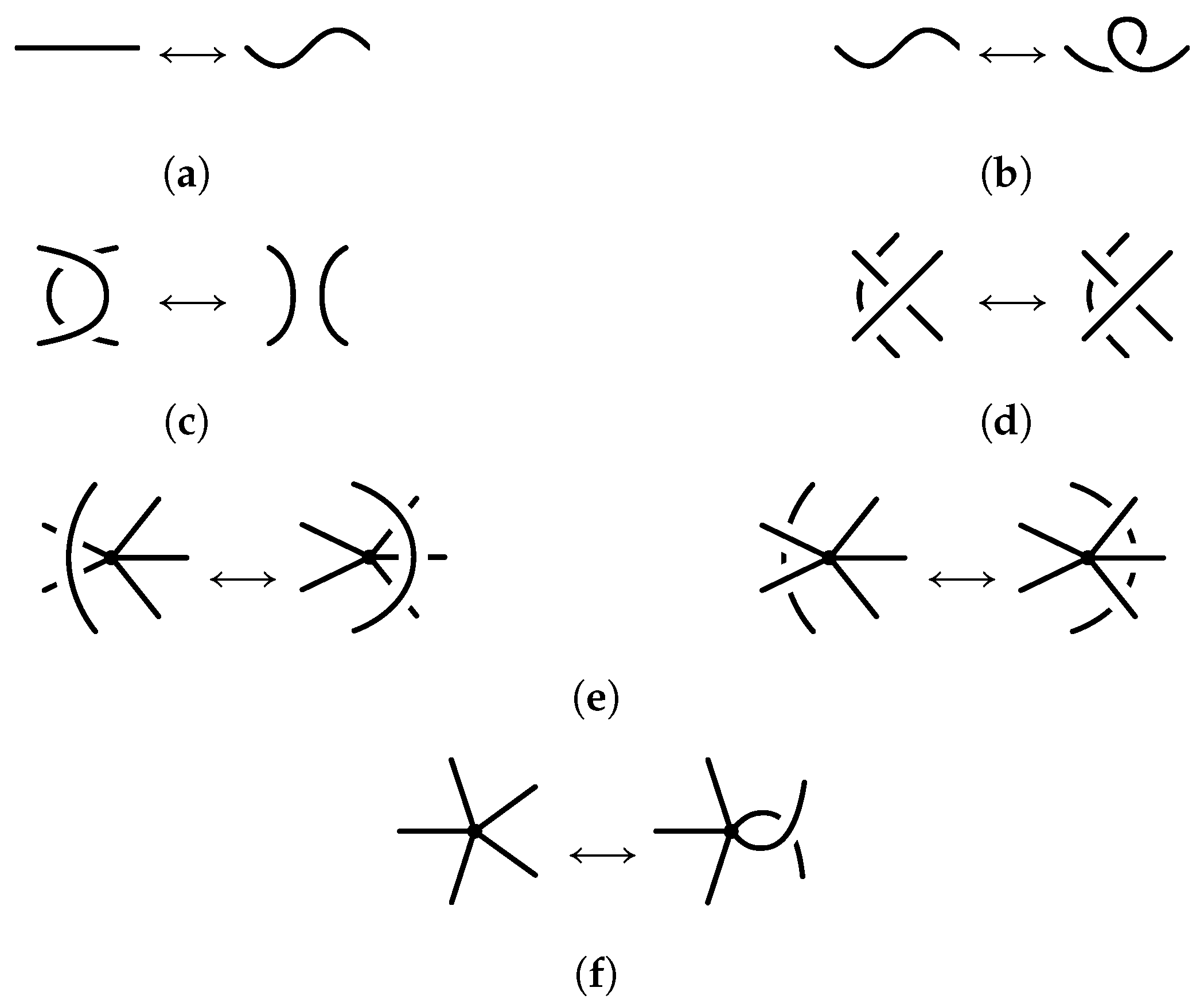
Definition 5. A contracted bond of a bonded knotoid diagram is a straight edge with two distinct trivalent vertices incident to it and without any interactions with itself or other strands of the diagram.
It is not hard to see that any bonded knotoid diagram can be transformed to a bonded knotoid diagram containing only contracted bonds. The transformations can be realized by pushing the bond vertices through intersecting strands via a sequence of bonded moves II and III. In
Figure 8, we illustrate a transformation of a bond into a contracted bond.
One can determine the tangle types to be utilized in tangle insertion according to the equivalence relation assumed for rigid bonded knotoid diagrams (
Figure 9).
Figure 10 shows that a rigid bonded type II move demands the inserted tangle to be isotopic to its horizontal reflection. A
rational tangle is a tangle that can be constructed by starting with two horizontal or two vertical strands, picking two endpoints and twisting them, then picking another pair and twisting them, and so on, for a finite number of twists [
12,
13]. Rational tangles are a good choice for tangle insertions since they are invariant under 180 degrees of vertical or horizontal rotation in the plane [
12]. With choices of rational tangles to be inserted in bonding sites, an equivalence between any two bonded knotoid diagram induces an equivalence between multi-knotoid diagrams resulting from the tangle insertion at the bonding sites of the bonded knotoid diagrams. This fact implies that a choice of tangle insertion into the nodes of a rigid vertex graph will give invariants of the graph from any invariants of the links obtained by the insertion.
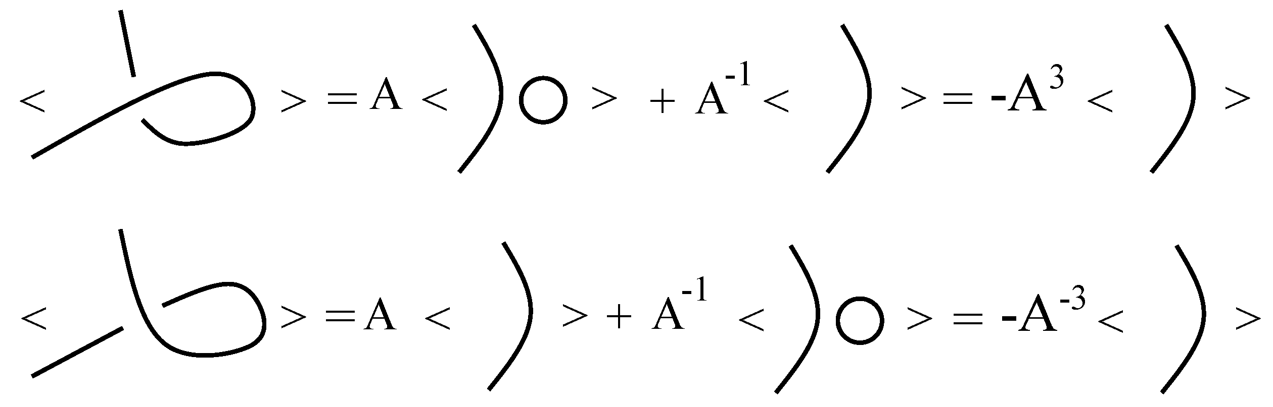
We utilize the Kauffman bracket expansion [
14] at the bonding sites to have the
double twist bracket polynomial. We do this first by inserting the
empty tangle, the
right-handed full twist tangle and the
left-handed full twist tangle at the bonding sites, where the inserted tangles are considered to be parallel to the neighboring strands of the bond. We then calculate the formal linear sum of the Kauffman bracket polynomials of the resulting knotoid diagrams, with formal coefficients
.
As we verify in
Figure 11, one crossing knotoid diagram with only one bond is non-trivial topologically, as its double twist bracket polynomial is non-trivial.
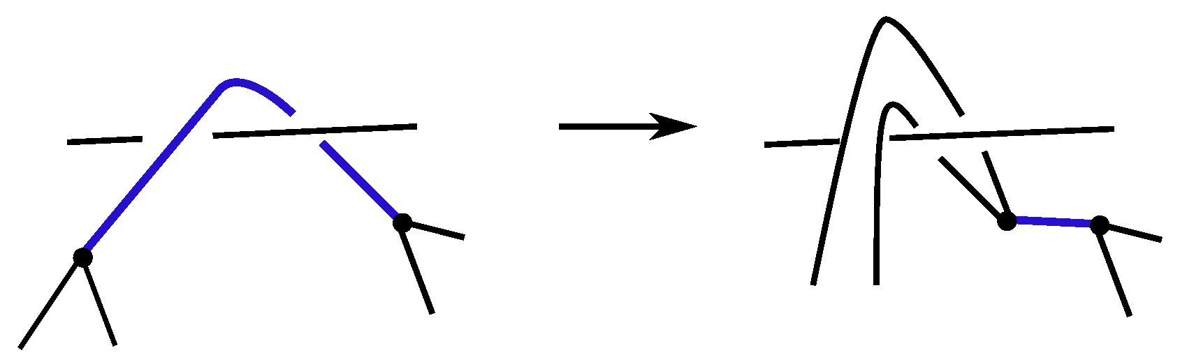
Proposition 1. The double twist bracket polynomial is a regular isotopy invariant of bonded (multi-)knotoids. That is, the double twist bracket polynomial is invariant under Reidemeister moves of type II and III but not of type I move.
Proof. In
Figure 12, we show the invariance under a rigid bond move of type II. The invariance under the other moves can be shown in a similar fashion. Adding a small curl to a bonded knotoid diagram by a type I Reidemeister move multiplies the double twist bracket polynomial of the diagram by
if the curl is right-handed and
if the curl is left-handed. See
Figure 13 for an illustration. □
Note that one can choose any rational tangle collection to be inserted at the bonding sites for the bracket expansion. In this way, we obtain an infinite collection of brackets induced by each choice of tangle insertion. None of the induced bracket polynomials is invariant under a R-I move, and this means that molecules that differ in writhe may have different invariants. One can
normalize a bracket polynomial as in [
14] to compensate for the writhe and induce a polynomial that is invariant under R-I, R-II and R-III moves.
Definition 6. The normalized double twist polynomial of an oriented (multi-)knotoid diagram K, is given as follows.
where
is the
writhe of
K, which is obtained by summing up the signs of crossings of
K.
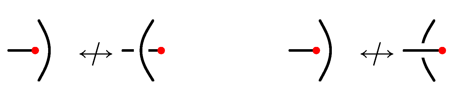
Oriented Case
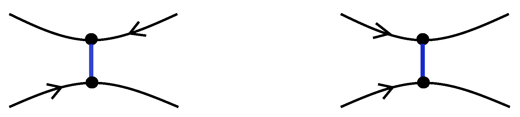
A knotoid diagram admits a natural orientation from one of its endpoints to the other one: conventionally from its tail to its head. The orientation on a bonded knotoid diagram induces two different types of oriented bonding sites, an
anti-parallel bonding site, where the orientation arrows on the local strands neighboring a bonded site are directed oppositely, and a
parallel bonding site, where the orientation arrows on the local strands neighboring a bonded site point to the same direction; see
Figure 14. Oriented bonded knotoid diagrams can be utilized to analyze open protein backbones that admit a natural orientation from one end (N-terminus) to the other end (C-terminus). Tangle insertion can be applied directly for oriented bonding sites by specific choices of rational tangles, and one can utilize knotoid invariants on the resulting oriented multi-knotoid diagram such as the arrow polynomial [
4,
7] and the affine index polynomial [
7,
15].
In [
4,
16], bonds of an oriented knot and knotoid diagram are interpreted as
rigid vertices that are graphical vertices admitting a determined cyclic order of its incident edges. This interpretation is provided by contracting an anti-parallel bonding site to a disoriented rigid vertex and a parallel bonding site to an
oriented rigid vertex with respect to the orientation on its incident edges. Then, to utilize topological invariants of knots or knotoids, each rigid vertex is replaced with certain rational tangles. We note here that our interpretation of bonds of oriented bonded knotoid diagrams coincides with the rigid vertex interpretation of bonds of an oriented bonded knotoid diagrams with a fixed collection of tangles to be used for tangle insertion; see
Figure 15. However, for unoriented bonded knotoid diagrams, the bond–rigid vertex correspondence is not one-to-one anymore, since vertical and horizontal bonds both are contracted to the same rigid vertex.
3.2. Invariants Induced by Unplugging
The unplugging invariant
T of spatial graphs was introduced in [
10], and in [
17], the invariant was extended to edge-colored spatial graphs. In this section, we extend this invariant to graphoids, edge-colored graphoids, and rail graphs. As a special case, it can be used to distinguish non-rigid bonded knotoids.
The unplugging invariant
T for graphoids is constructed as follows. At each vertex of a graphoid
G, we make a
local replacement as depicted in
Figure 16; for a vertex of degree
, there are
choices for a replacement. Note that the newly formed free ends are unmarked.
Let denote the multi-knotoid diagram formed by performing local replacements for each vertex, where we also remove all unknotted arcs, except if this arc contains both endpoints (marked vertices). We denote by the collection of multi-knotoids for all possible replacements .
Theorem 1. The set , whose elements are taken up to their multi-knotoid type, is an invariant of G.
Proof. The collection
is invariant under the Reidemeister moves, which is, as in the classical case [
10], easy to check. □
Given two graphoids,
and
, the sets
and
can be compared by any invariant of multi-knotoids, e.g., the Kauffman bracket polynomial or the Kauffman bracket skein module [
3].
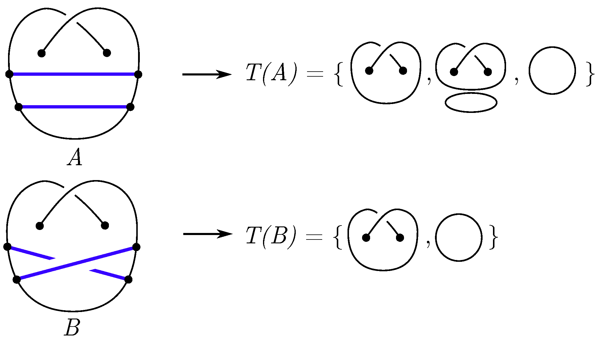
As an example, we compute the unplugging invariants for bonded knotoid diagrams
A and
B given in
Figure 17, which differ from each other by a bond swap. In [
3], it is shown that the Homflypt skein module of bonded links does not detect bond swaps; however, the unplugging invariants show that
A and
B are indeed different.
We can also consider
colored graphoids, i.e., a graphoid diagram
G together with a coloring function
where
is the set of edges of
G and
C is a set of colors; we will extend the unplugging invariant
T to a colored version, denoted by
(see also [
17] for a similar construction for generalized
-curves).
Let
a,
b, and
c be the colors of the edges incident to
v. We define a colored local replacement as a local replacement, where, in addition, we color each new arc by
, where
contains the colors of the preimage of the replacement according to the image in
Figure 18.
Similarly as before, denotes the colored multi-knotoid diagram formed by performing local replacements for each vertex, where we also remove all unknotted arcs, except if this arc contains both marked endpoints. We denote by the collection of multi-knotoids for all possible colored replacements .
Theorem 2. The set , whose elements are taken up to their multi-knotoid type, is an invariant of colored graphoids.
Proof. Again, invariance under Reidemeister moves is easy to check; see [
10,
17]. □
We can take the set of colors
and color the edges belonging to a non-rigid bonded knotoid diagram by 0 and the edges, belonging to the bonds, by 1. See
Section 4 for an example. Naturally, we can expand the coloring set if we want to distinguish different types of bonds.
3.3. Invariants Induced by Unpluggings of the Rail Closure
We associate to a bonded knotoid diagram
B a
long graphoid diagram , called the
rail closure of
B, by the following procedure: At each marked endpoint of
B, we draw a vertical line in the plane in such a way that the upper segment, starting from the endpoint, goes above the rest of the diagram, and the segment below the endpoint goes below the rest of the diagram, as depicted in
Figure 19 [
18]. The long graphoid diagram
corresponds to the diagram of the graphoid embedded in
-dimensional space
that is obtained by adding lines, perpendicular to the plane of
B, through each of the marked endpoints of
B.
Note that the equivalence between non-rigid bonded knotoid diagrams extends to the equivalence between rail closures, i.e., The unplugging invariant T is also well defined in the setting of rail closures, the resulting collection of a bonded knotoid diagram B is a set of long knots with possible multiple long arcs.
We conclude this section by giving some applications of rail closures.
In the first example, we consider the two knotoid diagrams
k and
in
Figure 20. The two non-trivial unpluggings (local replacements)
T and
of the rail closures
and
, respectively, represent mirror images of the long trefoil knot. Since the trefoil knot is chiral, we can conclude that
k and
are not equivalent.
In the second example, we demonstrate a verification that the bonded knotoid diagram
G given in
Figure 21 is not equivalent to the trivial bonded knotoid
H. If we take the rail closure of
G and perform a tangle insertion on one of the unpluggings by the horizontal empty tangle, we obtain a long link with linking number
, which we could not obtain if
G was equivalent to the trivial bonded knotoid diagram
H. It follows that
.
In the third example (
Figure 22), we show that the unplugging invariant of the rails of knotoids
k and
fails to detect they are not equivalent (see [
19], where it is shown that the parity bracket detects
). In the four-crossing unpluggings of the rail closures of the knotoids, we obtain the long figure eight knots
E and
. Since the figure eight knot is not chiral, we cannot conclude
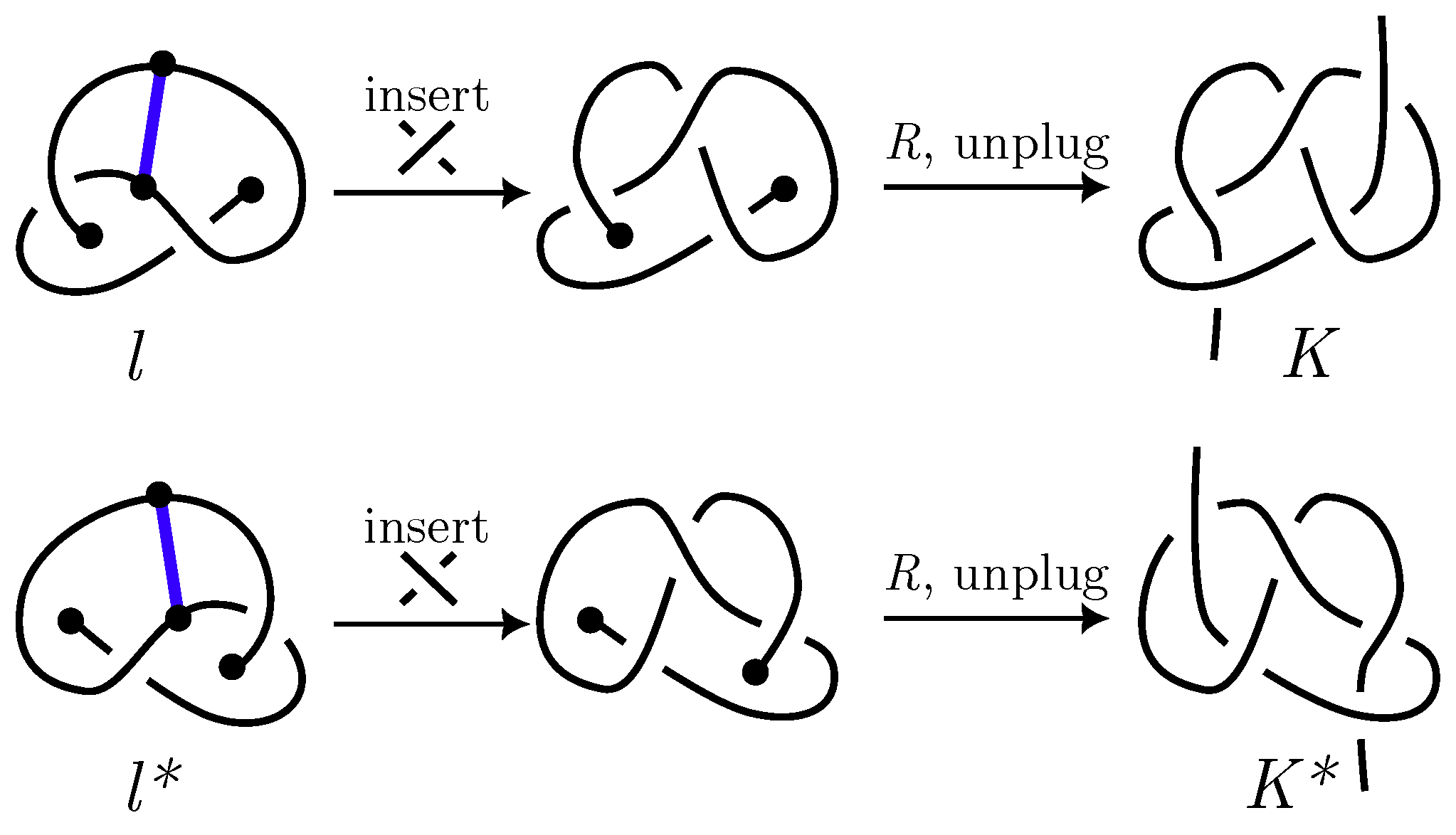
However, if we consider bonded knotoids
l and
, which correspond to knotoids
k and
after adding a bond (
Figure 23), perform a tangle insertion and consider the five-crossing unpluggings of the rail closures, we obtain two long chiral three-twist knots,
K and
, which are mirror images of each other. We can conclude
.


