Graph Mixed Random Network Based on PageRank

Abstract

In recent years, graph neural network algorithm (GNN) for graph semi-supervised classification has made great progress. However, in the task of node classification, the neighborhood size is often difficult to expand. The propagation of nodes always only considers the nearest neighbor nodes. Some algorithms usually approximately classify by message passing between direct (single-hop) neighbors. This paper proposes a simple and effective method, named Graph Mixed Random Network Based on PageRank (PMRGNN) to solve the above problems. In PMRGNN, we design a PageRank-based random propagation strategy for data augmentation. Then, two feature extractors are used in combination to supplement the mutual information between features. Finally, a graph regularization term is designed, which can find more useful information for classification results from neighbor nodes to improve the performance of the model. Experimental results on graph benchmark datasets show that the method of this paper outperforms several recently proposed GNN baselines on the semi-supervised node classification. In the research of over-smoothing and generalization, PMRGNN always maintains better performance. In classification visualization, it is more intuitive than other classification methods.

1. Introduction

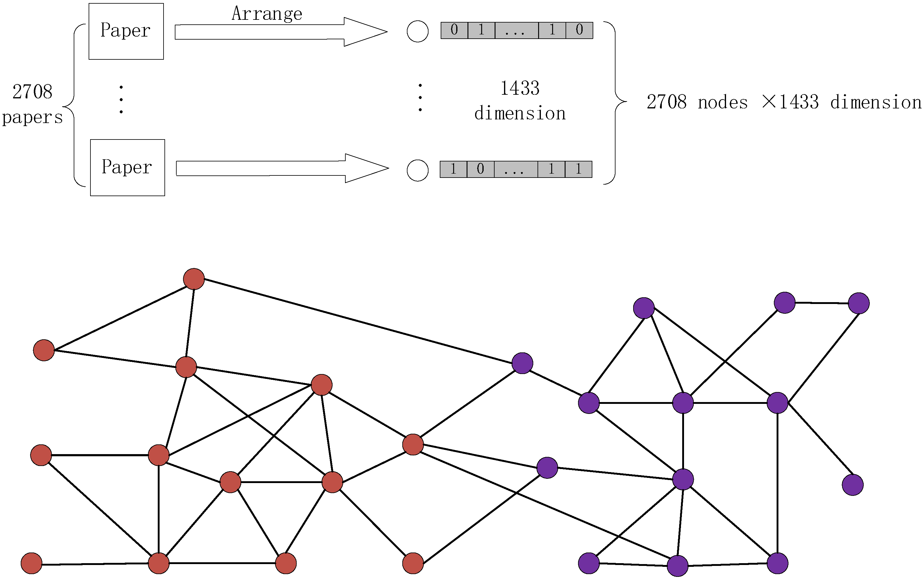
In the real world, graphs are ubiquitous and can be described in various forms. Graphs can be widely used in recommendation systems, citation networks, construction of protein structures in biochemistry, etc. Graph data is regarded as a carrier of information dissemination. As in Figure 1, the Cora dataset in the citation network is introduced. The Cora dataset consists of machine learning papers. It is a very popular dataset to use for graph deep learning in recent years. The papers are divided into a total of seven categories. In the final corpus, there are cited relationships between papers and papers. The lower part of Figure 1 shows this relationship with a graph data. There are 2708 papers in the entire corpus. After cataloging the papers, 1433 unique words are left to represent the papers. Cora dataset contains 1433 unique words, so the feature is 1433 dimensions. 0 and 1 in a single dimension describe whether each word exists in paper. In recent years, the research on learning from graph-structured data has received extensive attention in the field of machine learning and deep learning.

Semi-supervised node classification is one of the most popular and important problems in graph learning. In recent years, many effective node classification methods have been proposed by a wide range of scholars. In 2017, Kipf et al. proposed a new graph neural network structure, graph convolutional neural network (GCN) [1]. Standard GCNs learn the information of neighboring nodes, while Higher-Order Graph Convolution Architectures via Sparsified Neighborhood Mixing (MixHop) [2] can learn mixed neighbor relationships by repeatedly mixing feature representations of neighbors at different distances. Despite the great success of these algorithms, these models do not take full advantage of the relevant information about nodes and their neighbors.

The current hot topic focuses on the deformation of graph adjacency matrix. Yu Rong et al. proposed Towards Deep Graph Convolutional Networks on Node Classification (Dropedge) [3], an algorithm to randomly remove edges, and Dongsheng Luo et al. proposed Robust Graph Neural Network via Topological Denoising (PTDNet) [4] aiming to weed out task-irrelevant edges Both of the algorithms had low time complexity, but they did not benefit from added edges. Chen et al. [5] proposed to iteratively add (remove) edges among nodes with the same (different) labels while predicting. Although this approach increased the addition of edges, it depended heavily on the training size and was easy to make the error propagation. Recently Tong Zhao et al. proposed a Data Augmentation for Graph Neural Networks (GAUG) [6], a data augmentation method, which modified the structure of the graph by means of an edge predictor. It deleted unimportant edges, added possible data enhanced edges, and finally predicted the data with the modified edges.

Klicpera et al. [7] proposed a graph diffusion network (GDN), which coordinated spatial message passing and generalized graph diffusion, where diffusion acted as a denoising filter to allow messages to pass through higher-order neighborhoods. According to the different stages of diffusion, GDN can be divided into early fusion model and late fusion model. The early fusion model proposed by Xu et al. [8] and Jiang et al. [9] used graph diffusion to determine neighbors. For example, graph diffusion convolution (GDC) replaced the adjacency matrix in graph convolution with sparse diffusion matrix (Klicpera et al. [7]). The later fusion model (Tsitsulin et al. [10] and Klicpera et al. [11]) projected node features into a potential space, and then spread the learned node features.

In the aspect of the node classification task, how to fully use the large amount of unlabeled data becomes one of the important directions of research nowadays. Recently, in contrastive learning and unsupervised graph representation learning, Deep Graph Contrastive Representation Learning (GRACE) [12], Graph Contrastive Learning with Augmentations (GraphCL) [13] defined positive and negative pairs to maximize mutual information and expand data. In respect of the computer vision, Prototypical Contrastive Learning of Unsupervised Representations (PCL) [14], Exploring balanced feature spaces for representation learning (BalFeat) [15], and Unsupervised data augmentation for consistency training (UDA) [16] tried to make full use of unlabeled data for consistent regularization training to improve the generalization performance of the model. These ideas can be applied to the model to improve the performance of semi-supervised node classification.

The convolutional layers of GCN usually have only two layers, and the performance is higher when the layers are shallow, but gradually decreases as the layers become deeper. Li et al. [5] showed that the reason of over-smoothing was that by repeatedly applying the Laplacian smoothing, GCN might mix node characteristics from different clusters, making it difficult to distinguish. To solve the above problem, Jumping Knowledge Networks (JKNet) [17] alleviated the over-smoothing problem to some extent by combining the representation of each previous layer with the last layer. Wu et al. proposed Simplifying graph convolutional networks (SGC) [18], but it was still a shallow model and still had the risk of over-smoothing. Klicpera et al. proposed the Graph neural networks meet personalized pagerank (PPNP) [11] algorithm, which separated feature transformation from propagation and can aggregate multi-order neighbors without increasing the number of layers of the neural network.

By using a modified Markov diffusion kernel, Hao Zh et al. derived a variant of GCN named as Simple spectral graph convolution (SSGC) [19], which was able to balance the global and local information of each node. SSGC effectively utilized the information of the current node and its multi-order neighbors, while alleviating the over-smoothing problem.

How to effectively aggregate multi-order neighbors is still one of the current research focuses.

We propose the graph random neural network based on PageRank (PMRGNN), a simple and effective framework. Three approaches are used to solve the above problems: firstly, we design graph data augmentation for semi-supervised learning. Secondly, we extract features by combining two feature extractors. Finally, a graph regularization term is added to improve the performance of the designed model. The experimental results show that the PMRGNN can effectively improve the accuracy of node classification.

The rest of the paper is organized as follows: Section 2 presents the basic concepts of graph and semi supervised classification, and introduces the relevant models. Section 3 introduces the three modules of the proposed model and its basic theory, analyzing the algorithm and time complexity. The experimental design is presented in Section 4, and the obtained results are listed under Section 4. The conclusions and planned further work have been explained in the last section.

2. Concept and Related Work

2.1. Graph Concept

Given a simple undirected graph $G=(V,E)$, it consists of a $n$ nodes. As shown in Figure 2, for $G$, $A$ denotes the adjacency matrix, defining the interconnection between nodes, $A_{ij}=A_{ji}$. For each element of $A$, $A_{ij}=1$ indicates that there is an edge between nodes $v_i$ and $v_j$; $A_{ij}=0$ means there is no edge between the two.

2.2. Semi-Supervised Classification

The node characteristic matrix is $X$, $X\in R^{n\times d}$. $n$ is the number of nodes and $d$ is the dimension. For the node $v_i$, its feature vector is $X_i$, its label vector is $Y_i$, $Y\in R^{n\times C}$. $C$ represents the class of the node. The semi-supervised classification task is defined as follows:

Definition 1.

$m$labeled nodes $\left(0<m\le n\right)$, labeled as $Y^L$. $\left(n-m\right)$ unlabeled nodes, labeled as $Y^U$. Its purpose is to learn the prediction function $f:A,X,Y^L\to Y^U$ to infer $Y^U$ of unlabeled nodes.

In recent years, graph neural networks have become one of the most popular studies on semi-supervised node classification tasks. GNNs extend the neural networks techniques to graph, such as graph convolutional networks (GCNs). The propagation rule of a GCN is defined as:

$$H^{(l+1)}=\sigma \left(\widehat{A}{H}^{(l)}{W}^{(l)}\right).$$

(1)

where $\widehat{A}$ is the symmetric normalized adjacency matrix. $\widehat{A}={\widehat{D}}^{-1/2}\left(A+I\right){\widehat{D}}^{-1/2}$, and $\widehat{D}$ is the corresponding degree matrix of $A+I$. $\sigma$ represents the ReLU operation, $H^{\left(l\right)}$ and $W^{\left(l\right)}$ is the $l^{th}$ hidden layer node representation and weight matrix. $H^{\left(0\right)}=X$. The propagation of GCN is shown in the Figure 3. Under the semi-supervised classification task, $X_i$ gets $Z_i$ through the transformation of hidden layers, and $Z_i$ gets the prediction structure $Y_i$ through normalization.

2.3. Related Model

2.3.1. Diffusion Improves Graph Learning

Diffusion Improves Graph Learning (GDC) can be combined with any graph-based algorithm or model. GDC uses generalized graph diffusion, and the core of diffusion technology is $S={{\displaystyle {\sum }_{k=1}^{\infty }{\theta }_{k}T}}^k$, $T$ is the transfer matrix. According to different scenes, $T$ can be set as random walk transfer matrix and symmetric transfer matrix. $\theta$ of GDC can be personalized PageRank (PPR) [20] and heat kernel [21]. If $S$ represents the adjacency matrix and $D$ is the diagonal matrix of $S$, then the corresponding graph diffusion convolution is defined as $D^{-1/2}S{D}^{-1/2}x$, GDC eliminates the limitation of using only direct neighborhoods by introducing a powerful spatially localized graph convolution.

2.3.2. PPNP and APPNP

Klicpera et al. [11] proposed to use the Personalized PageRank to derive a fixed filter of order $K$. Let $f_{\theta }\left(X\right)$ represent the output of the two fully connected layers on the feature matrix $X$. PPNP is defined as:

$$H=\alpha {\left({\mathrm{I}}_n-\left(1-\alpha \right)\widehat{A}\right)}^{-1}{f}_{\theta }\left(\mathrm{X}\right).$$

(2)

To avoid computing the inverse ${\left({\mathrm{I}}_n-\left(1-\alpha \right)\widehat{A}\right)}^{-1}$, Klicpera et al. proposed the Approximate PPNP (APPNP) algorithm, which replaced the costly inverse with an approximation of truncated power iteration:

$$H^{(l+1)}=\left(1-\alpha \right)\widehat{A}{H}^{(l)}+\alpha H^{(0)}.$$

(3)

where $H^{(0)}$ = $f_{\theta }\left(x\right)$ = $ReLU\left(X\right)$ or $H^{(0)}$ = $f_{\theta }\left(x\right)$ = $\mathrm{MLP}(X)$. PPNP/APPNP separated feature transformation from propagation and aggregated information from multi-hop neighbors without increasing the number of layers in the neural network.

3. Model Analysis

3.1. PMRGNN Model

We first design a data augmentation method to achieve $S$ times graph data augmentation by a random propagation strategy (a). Then the basic framework which constitutes the network, a Mixed network structure (b), is introduced, as shown in Figure 4. In addition, a designed graph regularization term (c) is adopted, aiming to ensure the consistency between the node and its neighbor representation and improve the generalization ability under the semi-supervised setting. In this paper, the PMRGNN model is introduced in three directions: graph data random augmentation, Mixed network architecture, loss function and graph regularization term, respectively.

3.2. Random Augmentation of Graph Data

The model uses the method of masking features (MF), where the dimensions are randomly masked with zeros in the node features. Miller et al. [22] pointed out that neighbors were more likely to have similar feature representations or labels. Therefore, the information lost by the node can be compensated by its neighbors. The MF method is to randomly delete all feature elements of a single node. In other words, MF allows each node to aggregate information from a subset of its neighbors, ignoring some node properties, reducing reliance on specific neighbors while generating more random data.

As shown in Figure 5. First, we generate a binary mask ${\epsilon }_i$ for each node $v_i$. ${\epsilon }_i\sim Bernoulli(1-\delta )$. $\delta$ is the set hyperparameter. For the $i^{th}$ row vector of $X$, ${\tilde{X}}_i$=${\epsilon }_i\cdot X_i$. Then according to the generated matrix, we aggregate multi-order fields to produce multiple augmentation matrices, $\overline{X}=\tilde{A}\tilde{X},\tilde{A}={\displaystyle \sum {}_{k=0}^K}{\gamma }_k{\widehat{A}}^k$, where ${\gamma }_k=0,1,2\dots K$, ${\gamma }_k$ is the PageRank weight. ${\gamma }_k=\alpha {\left(1-\alpha \right)}^{k-1}$, $k=1,2\dots k-1$, ${\gamma }_K={\left(1-\alpha \right)}^{K-1}$, $\alpha$ is a hyperparameter. In the following experiment Section 4.4, We set ${\gamma }_k$ to learnable weight or ${\gamma }_k=1/\left(K+1\right)$. Experimental result shows the aggregation of multi-order neighbor-hood proposed in this paper is more effective. Compared with other models, the propagation rule contains more local information and is not overly parameterized while obtaining more distant information. $\tilde{A}$ is a dense matrix, which is difficult to compute in graph neural network. Therefore, by iteratively calculating the adjacency matrices ${\widehat{A}}^1$ to ${\widehat{A}}^k$$(1\le k\le K)$ with parameters ${\gamma }_k$, the enhanced feature matrix $\overline{X}$ is obtained. Repeat the above process for $S$ times to generate multiple enhanced characteristic matrices.

3.3. Mixed Network Architecture

In this paper, we use a network structure with a mixture of Multilayer Perceptron (MLP) and convolutional layers. It captures the key information between nodes, allowing the information of node and their neighbors to be used effectively. After random propagation for $S$ times, $S$ feature matrices is generated, $\left(1\le s\le S\right)$. We feed each augmented feature matrix into the designed neural network. The mixed network structure is defined as follows:

$$H_{(s)}^{(l+1)}=\sigma \left(\alpha \left(H_{(s)}^{(l)}{W}_1{}^{(l)},\widehat{A}{H}_{(s)}^{(l)}{W}_2{}^{(l)}\right)\right),$$

(4)

$${\tilde{Z}}^{\left(s\right)}=f_{PMRGNN}{}^{\left(l\right)}\left(\widehat{A},{\overline{X}}^{\left(s\right)},\theta \right).$$

(5)

Equation (4), represents a matrix of $n$ nodes and $k$-dimensional representations on the $l^{th}$ layer generated by the feature matrix ${\overline{X}}^{(s)}$$H_{(s)}^{(l)}\in {\mathrm{R}}^{n\times k}$, $H_{(s)}^{(0)}={\overline{X}}^{\left(\mathrm{s}\right)}$. $\alpha$ is an aggregation function, which can be spliced or added. Its purpose is to aggregate the hidden representation of adjacent nodes. $W_1{}^{(l)},W_2{}^{(l)}\in R^{k\times k^{\prime }}$, are linear transformation matrices. $k^{\prime }$ represents the ${\left(l+1\right)}^{th}$ dimension. $\sigma$ is a nonlinear activation function, such as the ReLU. Equation (5), ${\tilde{Z}}^{\left(s\right)}$ is the output of the mixed network layers, ${\tilde{Z}}^{\left(s\right)}\in R^{n\times C}$. $\theta$ is PMRGNN weights. ${\tilde{P}}^{(s)}$ represents the node classification probability predicted from ${\tilde{Z}}^{\left(s\right)}$. ${\tilde{P}}^{(s)}\in {[0,1]}^{n\times \mathrm{C}}$, ${\tilde{P}}^{(s)}=softmax({\tilde{Z}}^{\left(s\right)})$. A single feature extractor may not be able to fully capture the key information between nodes.

The two feature extractors are MLP and GCN for convolutional layers The method of combining two different feature extractors proposed in this paper can effectively utilize the information of node and their neighbors. The algorithm Improved Training of GNNs (GraphMix) [23] proposed by Vikas et al. is similar to us. It is trained by a fully-connected network jointly with the graph neural network via parameter sharing and interpolation-based regularization.

In Section 4.3, the case of using MLP and GCN alone is compared. Experiment shows using a combination of MLP and GCN layers has better experimental results than using them alone.

3.4. Loss Function and Regularization Term

In traditional graph semi-supervised learning, the loss function contains supervision loss on labeled nodes and graph regularization loss [24,25].

3.4.1. Supervision Loss

In this paper, the loss includes three parts: the supervised loss, the feature extractor loss to measure the prediction results between MLP and GCN layers, and the graph regularization loss.

${\tilde{P}}^{(s)}$ represents the node classification probability predicted from ${\tilde{Z}}^{\left(s\right)}$. In a graph, there are $m$ labeled nodes out of $n$ nodes. The average cross-entropy loss generated by $S$ augmented matrices is defined as:

$$L_{sup}=-{\displaystyle \sum _{s=1}^S{\displaystyle \sum _{i=0}^{m-1}{\mathrm{Y}}_i^{\mathrm{T}}}}\log {\tilde{P}}_i^{(s)}.$$

(6)

3.4.2. Feature Extractors Loss

The output result of the MLP is $Z^{(f)}$, and the output result of the GCN layers is $Z^{(g)}$. We use KL divergence to minimize the distance between the two feature extractors, making efficient use of node and its neighbor information:

$$L_{KL}={\displaystyle \sum _{i=1}^N{\displaystyle \sum _{j=1}^C{Z}_{{}_{ij}}^{(f)}}}\log \frac{Z_{ij}^{(f)}}{Z_{ij}^{(g)}}.$$

(7)

3.4.3. Graph Regularization Term

In traditional semi-supervised node classification learning, the graph Laplacian regularization term is usually used to provide the model $f(x,\theta )$ with graph structure information. With the increasing popularity of GNNs in recent years, applying adjacency matrices $A$ to the models $f\left(A,X,\theta \right)$ has become a more common method. Meiqi zhu et al. [26] pointed out that prediction function in GNN had a Laplacian regularization term. Therefore, it was unnecessary to add a traditional graph Laplacian regularization term to the existing GNN. We use a simple and effective variant of Laplacian regularization to improve the performance of existing GNN model ${\tilde{P}}_{ij}^{(s)}$ is the predicted probability of the node $i$ in the class $j$, ${\tilde{P}}_{ij}^{(s)}=\exp ({\tilde{Z}}_{ij}^{(s)})/{\displaystyle {\sum }_{k=1}^C\exp ({\tilde{Z}}_{ik}^{(s)})}$. By further propagating, ${\tilde{Z}}_{ij}^{(s){}^{\prime }}=\widehat{A}{\tilde{Z}}_{ij}^{(s)}$. we obtain the cross-entropy ${\tilde{Q}}_{ij}^{(s)}=\exp ({\tilde{Z}}_{ij}^{(s){}^{\prime }})/{\displaystyle {\sum }_{k=1}^C\exp ({\tilde{Z}}_{ik}^{(s){}^{\prime }})}$. The regularization term defined in this paper is:

$$L_{reg}=\frac{1}{N}{\displaystyle \sum _{s=1}^{\mathrm{S}}\phi \left({\tilde{Z}}^{\left(s\right)},\widehat{A}{\tilde{Z}}^{\left(s\right)}\right)},$$

(8)

$$\phi =-{\displaystyle \sum _{i=1}^N{\displaystyle \sum _{j=1}^C{\tilde{P}}_{ij}^{(s)}\log {\tilde{Q}}_{ij}^{(s)}}},$$

(9)

$$\phi =\frac{1}{2}{{\displaystyle \sum _{i=1}^N\left|\left|{\left(\widehat{A}{Z}^{(s)}\right)}_i^T-{\left(Z^{(s)}\right)}_i^T\right|\right|}}_2^2.$$

(10)

$\phi$ is a function to measure the degree of difference between two features, which can be measured by the cross-entropy (9) or the squared error (10). The purpose of adding $\phi$ is to measure the similarity of the same node in different propagation processes. At the same time, $\phi$ makes the node similar to its neighbor representation during optimization. Laplace regularization term is edge centered:

$$L_{lap}={\displaystyle \sum {}_{\left(i,j\right)\in E}}\left|\left|Z_i^T-Z_j^T\right|\right|.$$

(11)

In this paper, the regularization term is node centered:

$$\phi \left(Z,\widehat{A}Z\right)={\displaystyle \sum _{i=1}^N\phi \left(Z_i^T,{\left(AZ\right)}_i^T\right)}.$$

(12)

Han et al. [27] proposed that if the number of GCN layers approached infinity, each node can capture and represent the information of the whole graph, i.e., $\tilde{Z}=A^{\infty }Z$, ${\tilde{z}}_1=\dots ={\tilde{z}}_N$. Infinite layer convolution has a similar effect to minimizing the square error of the characteristic matrix (10). Minimizing the square error of the characteristic matrix in the training process generates the same output vector for each node, i.e., $\tilde{Z}\in \arg {\min }_Z{\left|\left|\widehat{A}Z-Z\right|\right|}_F^2$,

$${\left|\left|\widehat{A}Z-Z\right|\right|}_F^2={\left|\left|\left(D^{-1}A-I\right)Z\right|\right|}_F^2={{\displaystyle \sum _{i=1}^N\left|\left|\left(\frac{1}{d_i}{\displaystyle \sum _{j\in N(v_i)}{z}_j}\right)-z_i\right|\right|}}_2^2.$$

(13)

$d_i$ represents the degree of node $v_i$, and $N_{(i)}$ represents the neighbor of node $v_i$. If Equation (10) is minimized iteratively, then:

$$z_i^{(k+1)}=\frac{1}{d_i}{\displaystyle \sum _{j\in N(v_i)}{z}_j^{(k)}}.$$

(14)

where $k$ is the number of iteration steps, then the graph convolution of $z_i^{(k)}$ is:

$$z_i^{(k+1)}={\displaystyle \sum _{j\in N(v_i)}\frac{1}{\sqrt{d_i{d}_j}}{z}_j^{(k)}}.$$

(15)

It can be seen that (14) and Equation (15) are similar. When $k\to +\infty$, both converge to a certain point, i.e., $Z^{(k+1)}=\widehat{A}{Z}^{(k)}$. Therefore, minimizing the square error of the characteristic matrix is similar to using infinite convolution on a graph. The traditional Laplacian regularization term only shortens the distance between the target node and the neighbor node. Equation (14) is similar to using the voting results of each node’s neighbors to represent the target node, providing additional classification information for the node. In this paper, we use graph regularization term to capture more information for the model.

3.4.4. Final Loss

Final loss contains: the supervised loss (6), the feature extractors loss (7) and the graph regularization term (8). During epoch of training, the parameters are updated using the final loss. ${\lambda }_1$ and ${\lambda }_2$ are the hyperparameters controlling the balance of the loss. The hyperparameter ${\lambda }_1$ is to control the feature extractors loss (7). The hyperparameter ${\lambda }_2$ is to control the graph regularization term (8). This paper uses ${\lambda }_1$ and ${\lambda }_2$ to balance the final loss:

$$L=\frac{1}{S}{L}_{\sup }+{\lambda }_1{L}_{KL}+{\lambda }_2\frac{1}{S}{L}_{reg}.$$

(16)

In summary, the training process of the PageRank-based graph mixed random network is shown in Algorithm 1.

Algorithm 1: PMRGNN

Input: Adjacency matrix $\widehat{A}$; feature matrix $X$; propagation step $S$; mask matrix ratio $\delta$; PageRank weight $\alpha$; $f_{MLP}\left(X,\theta \right)$; $f_{GCN}\left(A,X,\theta \right)$; $f_{PMRGNN}\left(A,X,\theta \right)$.

Output: Trained PMRGNN weights $\theta$, Prediction $P$.

while the not convergence do

for $s=1:S$ do

Generate binary mask ${\epsilon }_i$ for each node $v_i$:

${\epsilon }_i\sim Bernoulli(1-\delta )$

Masking feature: ${\tilde{X}}_i^{(s)}={\epsilon }_i\cdot X_i$

Propagation based on PageRank:

${\overline{X}}^{(s)}=\tilde{A}{\tilde{X}}^{(s)}$,$\tilde{A}={\displaystyle {\sum }_{k=0}^K{\gamma }_k{\widehat{A}}^k}$

Generate node embedding:

${\tilde{Z}}^{(s)}=f_{PMRGNN}\left(\widehat{A},{\overline{X}}^{(s)},\theta \right)$

Propagation again: ${\tilde{Z}}^{(s){}^{\prime }}=\widehat{A}{\tilde{Z}}^{(s)}$

end for

Generate node embedding using MLP:

$Z^{(f)}=f_{MLP}\left(X,\theta \right)$

Generate node embedding using GCN:

$Z^{(g)}=f_{GCN}\left(A,X,\theta \right)$

Calculate Kl regularization term: (7)

Generate graph regularization term: (8)

Calculate supervision loss: (6)

Calculate total loss: (16)

Update the model weight $\theta$ according to the

gradient descent method.

end while

return PMRGNN weights $\theta$, Prediction $P$.

3.5. Time Complexity Analysis

In the random augmentation of graph data, the time complexity is $O\left(Kd\left(n+\left|E\right|\right)\right)$, where $K$ is the propagation steps, $d$ is the feature dimension of nodes, $n$ is the number of nodes, and $\left|E\right|$ is the number of edges. In this paper, we use a network structure with a mixture of Multilayer Perceptron (MLP) and convolutional layers. The time complexity of the MLP is $O\left(n{d}_h\left(d+C\right)\right)$; The time complexity of convolutional layers is $O\left(\left|E\right|d_h\left(d+C\right)\right)$, $d_h$ represents the hidden layer dimension, and $C$ represents the number of classes. When calculating the loss function, we need to consider the graph regularization term. By sparse-dense matrix multiplication or message passing framework (Glimer et al. [28]), it is proved that the time complexity of calculating $\widehat{A}{\tilde{Z}}_{ij}^{(s)}$ is $O\left(\left|E\right|C\right)$, and the time complexity of calculating $\phi$ is $O\left(nC\right)$. Finally, we come to the conclusion that the time complexity of graph regularization term is $O\left(\left|E\right|C+NC\right)$. In this paper, a total of $S$ random augmentations of graph data are made on the graph, so the total time complexity of the model is:

$$O\left(S\left(Kd\left(n+\left|E\right|\right)+\left(\left|E\right|+n\right)d_h\left(d+C\right)+\left|E\right|C+nC\right)\right).$$

(17)

4. Experiment and Analysis

In order to verify the performance of the proposed model, we conduct experiments on three general benchmark datasets and compare it with baseline models. In Section 4.1, the benchmark datasets and the baseline models are introduced. In Section 4.2, the PMRGNN is compared with the baseline models. In Section 4.3, we conduct the ablation experiment to understand the contribution of each component to functionality. In Section 4.4, We compare the weight of ${\gamma }_k$ for PageRank with other cases. In Section 4.5, the generalization performance of the model is analyzed. In Section 4.6, at low labeling rate, we analyzed the PMRGNN model and other GNN baselines. In Section 4.7, the experiments of over-smoothing are analyzed. In Section 4.8, We perform a visual analysis of the classification of two GNN baselines and PMRGNN.

4.1. Data Sets and Benchmark Algorithm(s)

In this paper, we conduct experiments on three benchmark graphs [1,29]: Cora, CiteSeer and PubMed. The specific information of the datasets is shown in

Table 1. Dataset Statistics.

Dataset	Nodes	Features	Edges	Classes	Labeling Rate
Cora	2708	1433	5429	7	0.052
CiteSeer	3327	3700	4732	6	0.036
PubMed	19,717	500	44,338	3	0.003

.

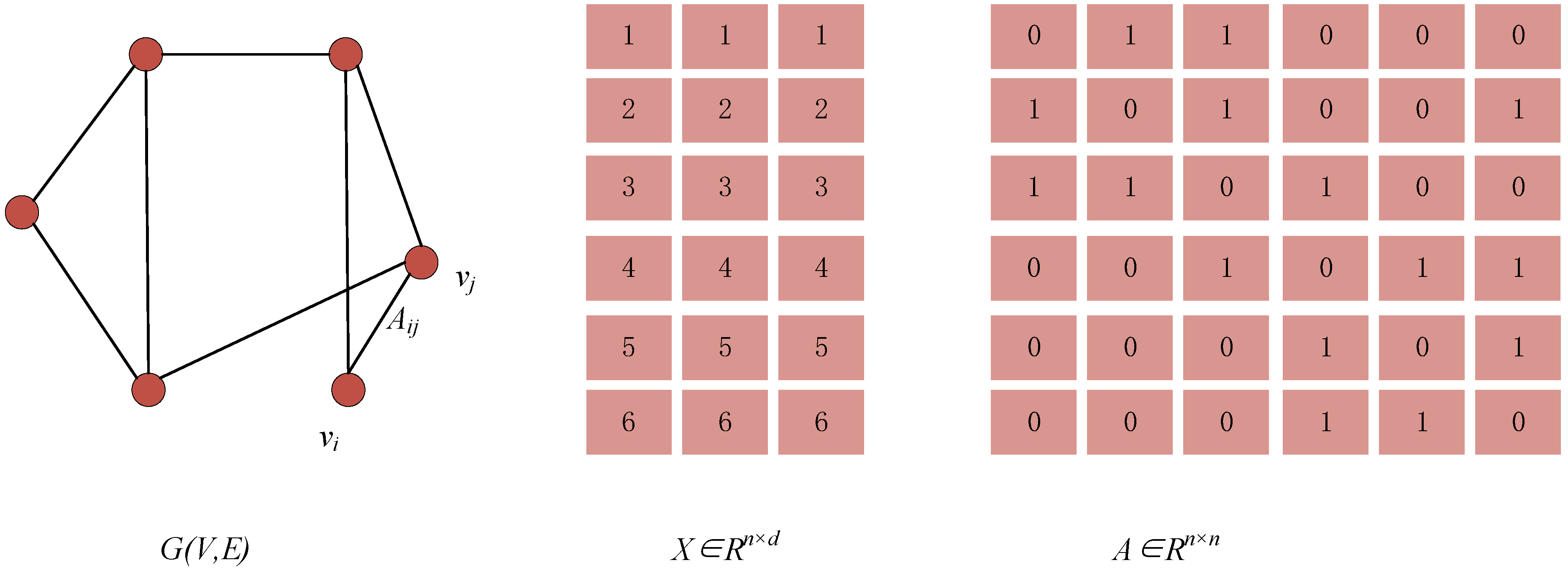
The experimental setup of Yang et al. [30] is used in the experiment. In the citation network datasets, the nodes are documents to form the feature matrix $X$. The citation links are regarded as the undirected edges and can be constructed as an adjacency matrix $A$. The training set consists of 20 nodes in each class, 500 nodes verification set and 1000 nodes test set. The labeling rate is the ratio of labelled nodes to the total nodes in the dataset. Its formula is $(classes\times 20)/nodes$. For example, the labeling rate of Cora is $\left(7\times 20\right)/2708=0.052$.

Baseline models: eight different neural networks are selected as baseline models, Graph convolutional networks (GCN) [1], Graph attention networks (GAT) [29], Simplifying graph convolutional networks (SGC) [18], Graph neural networks meet personalized pagerank (APPNP) [11], Towards Deep Graph Convolutional Networks on Node Classification (DropEdge) [3], Adaptive universal generalized PageRank graph neural network (GPRGNN) [31], Simple spectral graph convolution (SSGC) [19], Simple and deep graph convolutional networks (GCNII) [32]. A GNN based sampling method: Inductive representation learning on large graphs (GraphSAGE) [33].

4.2. Experimental Results

The prediction accuracy of node classification is summarized in

Table 2. Accuracy Rate of Standard Classification.

Method	Cora	CiteSeer	PubMed
GCN	81.5	70.3	79.0
GAT	$80.3\pm 0.7$	$72.5\pm 0.7$	$79.0\pm 0.3$
SGC	$81.0\pm 0.0$	$81.9\pm 0.1$	$78.9\pm 0.0$
DropEdge	$81.8\pm 0.8$	$71.9\pm 0.2$	$79.1\pm 0.3$
APPNP	$83.7\pm 0.5$	$71.5\pm 0.3$	$79.3\pm 0.5$
GPRGNN	$82.5\pm 0.4$	$71.1\pm 0.6$	$79.4\pm 0.8$
GraphSAGE	$81.6\pm 0.6$	$70.2\pm 0.7$	$78.3\pm 0.3$
SSGC	$82.6\pm 0.1$	$73.0\pm 0.0$	$80.0\pm 0.1$
GCNII	$84.9\pm 0.4$	$72.9\pm 0.5$	$80.2\pm 0.4$
PMRGNN	$85.2\pm 0.2$	$75.3\pm 0.3$	$80.4\pm 0.2$

. The comparison experiment methods are the baseline models used in Section 4.1. The result of PMRGNN is average value of 50 runs with random weight initialization.

In Table 2, it can be noticed that the PMRGNN proposed in this paper is superior to the compared baseline models. Specifically, compared with GCN, our strategy performance improves by 3.7%, 5.0% and 1.4% in Cora, CiteSeer and PubMed. Compared with GAT, it increases by 2.2%, 2.8% and 1.4%. Compared with GCN, SSGC raises by 1.1%, 2.7% and 1.0%. Compared with GCN, GCNII is improves by 3.4%, 2.6% and 1.2%. Our strategy is 0.3%, 2.4% and 0.2% higher than GCNII.

4.3. Ablation Experiment

We conduct an ablation experiment to understand the contributions of different components in PMRGNN.

Unshielded feature (w/o MF): remove mask matrix, just use DropNode.

Neural network structure setting MLP (net-MLP): the combination of two feature extractors is changed to use MLP alone.

Neural network structure setting GCN (net-GCN): the combination of the two feature extractors is changed to use GCN alone.

No Feature extractors loss (w/o KL loss): There is no KL loss in the final loss.

No regularization term (w/o reg): remove the graph regularization term, and set the super parameter of the graph regularization term as 0.

In

Table 3. Accuracy Rate of Ablation Experiment.

Method	Cora	CiteSeer	PubMed
w/o MF	$84.7\pm 0.2$	$74.7\pm 0.2$	$79.6\pm 0.1$
net-MLP	$84.8\pm 0.2$	$74.8\pm 0.5$	$79.9\pm 0.3$
net-GCN	$84.2\pm 0.4$	$74.5\pm 0.3$	$79.4\pm 0.6$
w/o reg	$84.2\pm 0.2$	$73.2\pm 0.5$	$79.7\pm 0.3$
w/o KL loss	$84.3\pm 0.2$	$74.7\pm 0.3$	$79.7\pm 0.2$
PMRGNN	$85.2\pm 0.2$	$75.3\pm 0.3$	$80.4\pm 0.2$

, We summarize the results of the ablation experiment. After removing some components from PMRGNN, it can be observed that the performance will be reduced comparing with the complete model, indicating that the components designed in this paper can help to improve the accuracy of the model. Table 3 shows that masking features produces random data augmentation; using one feature extractor alone is not as effective as using two feature extractors in combination; At the same time, the graph regularization can effectively improve the performance of the model.

4.4. PageRak Weight Comparison Experiment

In this paper, we design a multi-level domain with aggregation nodes: $\overline{X}=\tilde{A}\tilde{X}$,$\tilde{A}={\displaystyle {\sum }_{k=0}^K{\gamma }_k{\widehat{A}}^k}$, parameter ${\gamma }_k$ is the PageRank weight. In this section, we compare the case where ${\gamma }_k$ is the learnable weight or ${\gamma }_k=1/\left(K+1\right)$. Experimental results show that the method of aggregating multi-order neighborhoods proposed in this paper is more effective (as shown in

Table 4. Comparison of Different Weights.

Method	Cora	CiteSeer	PubMed
with learn	$83.7\pm 0.1$	$74.0\pm 0.2$	$78.2\pm 0.2$
with 1/(K + 1)	$84.8\pm 0.4$	$74.9\pm 0.2$	$79.9\pm 0.3$
with pagerank	$85.2\pm 0.2$	$75.3\pm 0.3$	$80.4\pm 0.2$

).

4.5. Generalization Performance Analysis

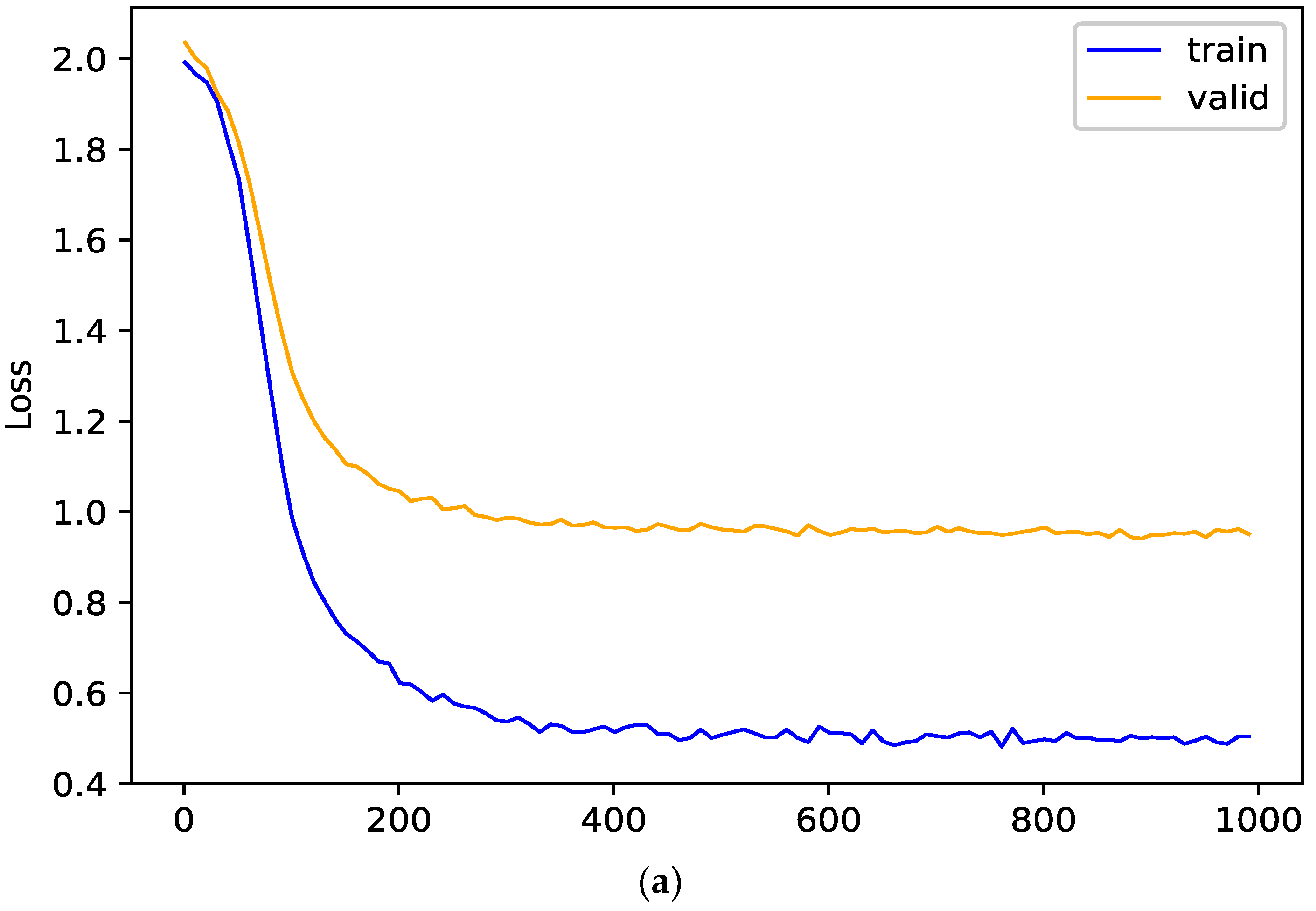
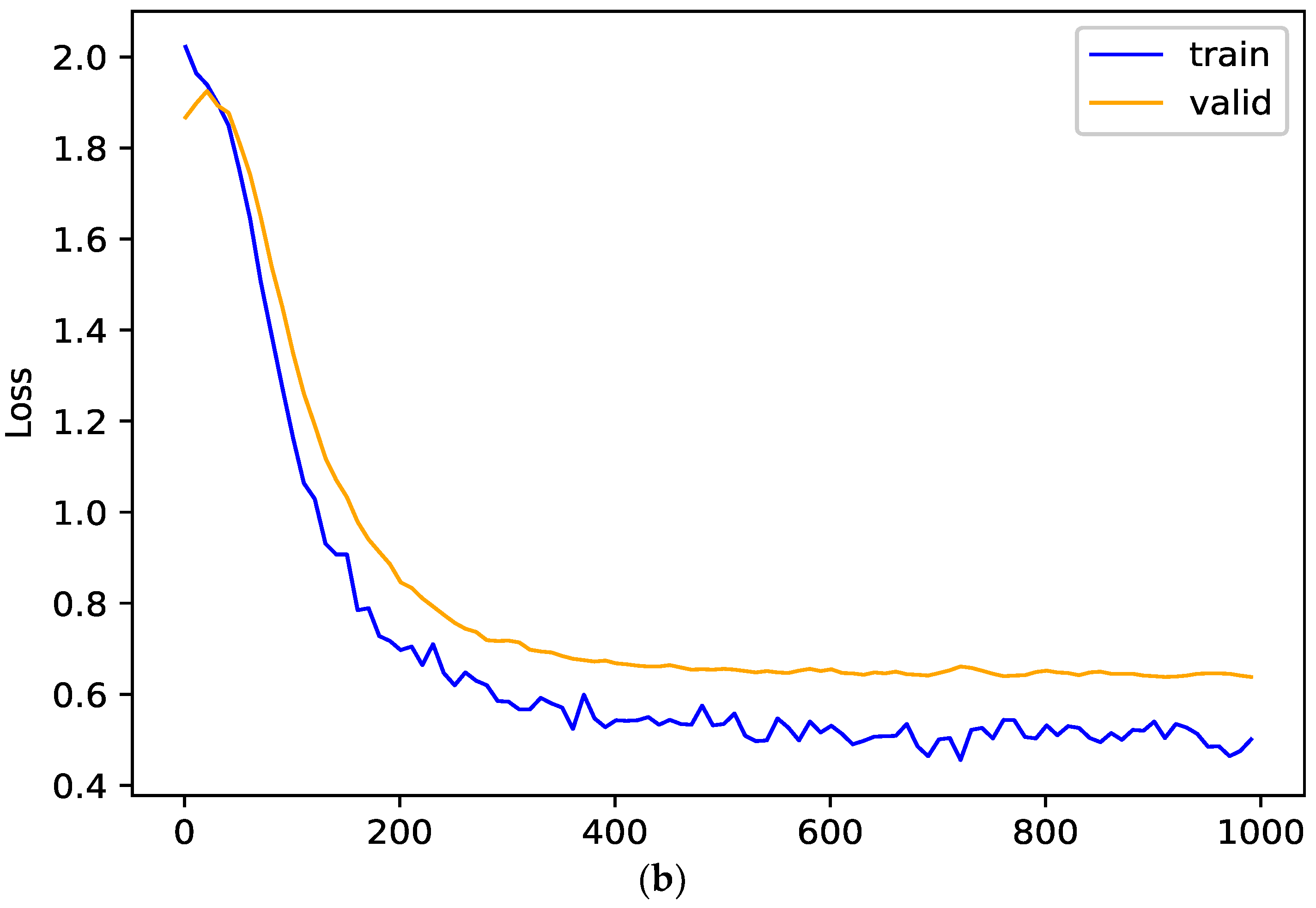
In this section, the effects of random propagation and graph regularization term on the generalization ability of the model are studied. In order to verify their effects on the model, the training loss and verification loss of the model on Cora dataset are analyzed. The smaller the gap is between the two losses, the better the generalization performance of the model is. The generalization performance of the model and its variant (w/o reg) are shown in Figure 6. When there is no graph regularization term, an obvious gap between the training loss and the verification loss can be observed in the Figure 6a; When the graph regularization term is added, the verification loss is close to the training loss in the Figure 6b. These show that the graph regularization term added in this paper can improve the generalization performance of PMRGNN.

4.6. Low Label Rate Experiment

In order to verify the performance of PMRGNN, we conduct experiments on datasets with lower label rate. The result statistics are shown in

Table 5. Accuracy Rate of Standard Classification.

Method	Cora	CiteSeer	PubMed
GCN	$73.2\pm 2.6$	$63.2\pm 2.3$	$73.0\pm 2.9$
GAT	$77.0\pm 2.1$	$66.3\pm 2.2$	$72.8\pm 2.2$
SGC	$71.3\pm 3.4$	$66.0\pm 2.3$	$73.6\pm 3.2$
DropEdge	$73.0\pm 2.9$	$64.0\pm 3.1$	$73.5\pm 2.3$
APPNP	$77.9\pm 2.4$	$66.1\pm 2.4$	$74.4\pm 3.9$
GPRGNN	$78.4\pm 1.7$	$63.7\pm 3.0$	$74.4\pm 2.8$
GraphSAGE	$75.6\pm 2.2$	$65.4\pm 2.2$	$73.6\pm 4.0$
SSGC	$78.1\pm 1.8$	$66.0\pm 2.6$	$73.1\pm 3.0$
GCNII	$75.6\pm 1.2$	$68.3\pm 1.1$	$73.2\pm 2.2$
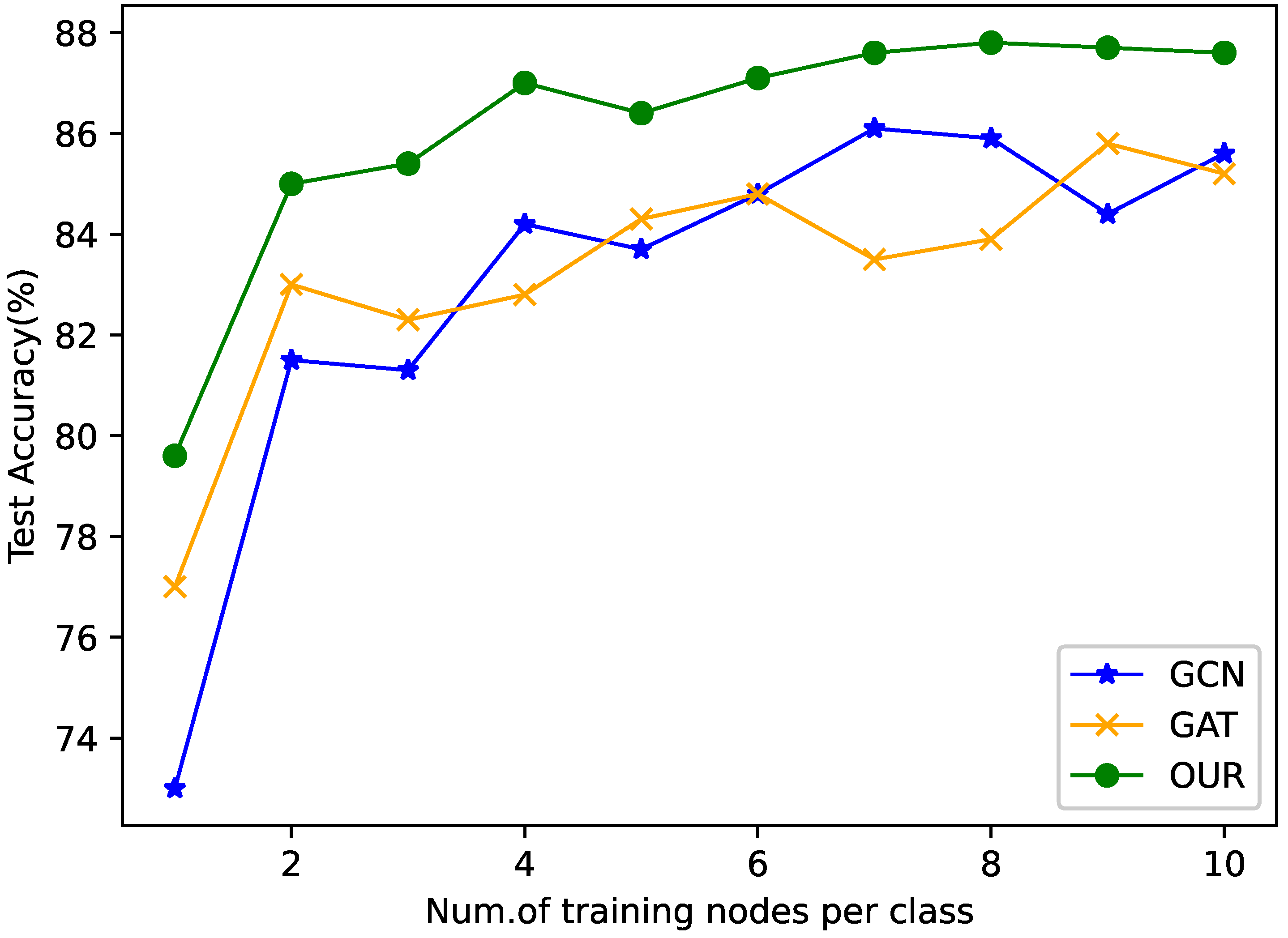
PMRGNN	$79.6\pm 1.4$	$68.6\pm 3.1$	$74.7\pm 3.1$

. The training set contains 10 nodes of each class, the validation set contains 500 nodes, and the test set contains 1000 nodes. On the datasets with lower label rate, the performance of our strategy is still at a higher level than other models. Specifically, the model has improved by 6.4%, 5.4% and 1.7% compareing with GCN on Cora, CiteSeer and PubMed datasets. Compared with GAT, it increases by 2.6%, 2.3% and 1.9%. PMRGNN is 1.2%, 0.3% and 0.3% higher than the best algorithm on each dataset.

Figure 7 shows the comparison of the accuracy of Cora dataset on different training sets (each type of trained nodes ranges from 10 to 100). It can be observed that the algorithm designed in this paper is generally higher than GCN and GAT in all partitions.

4.7. Over-Smoothing Experiment

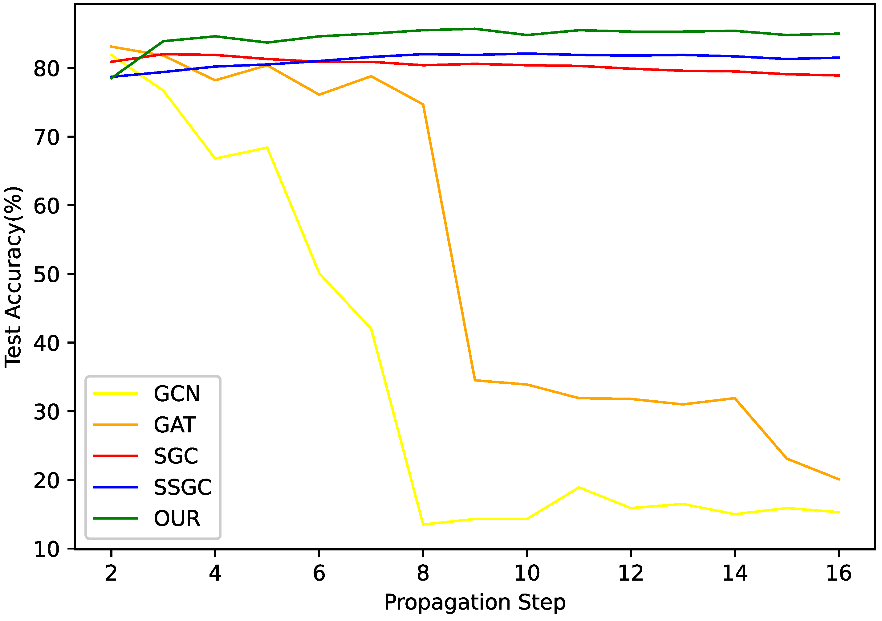
Many GNNs are faced with the problem of over-smoothing when the step size of feature propagation is enlarged. When the propagation step size increases, the nodes with different labels will become difficult to distinguish. In order to verify the ability of PMRGNN to alleviate the problem of over-smoothing, we conduct an experiment on the Cora dataset with different propagation steps.

Figure 8 shows the experimental results on the Cora dataset. The propagation step length in PMRGNN is controlled by the super parameter $k$. The hyperparameter $k$,$k\in \left\{0,\dots 14\right\}$ is the number of propagation steps of the adjacency matrix in augmentation of graph data. In Section 3.2, the hyperparameter $k$ is reflected in $\tilde{A}={\displaystyle \sum {}_{k=0}^K}{\gamma }_k{\widehat{A}}^k$. For GCN and GAT, they are adjusted by superimposing different hidden layers. For SGC and SSGC, the propagation depth of data preprocessing is adjusted. The experimental results show that with the increase of propagation step length, the indexes of GCN and GAT decrease significantly. Due to the problem of over-smoothing, the accuracy of GCN decreases from 81.5% to 15%, the accuracy of GAT reduces from 83% to 20%. PMRGNN, SGC and SSGC can alleviate the problem of over-smoothing. They can be stabilized within a certain range. But our method performs better. Compared with other algorithms, the accuracy of PMRGNN is always the highest, maintained at 85%.

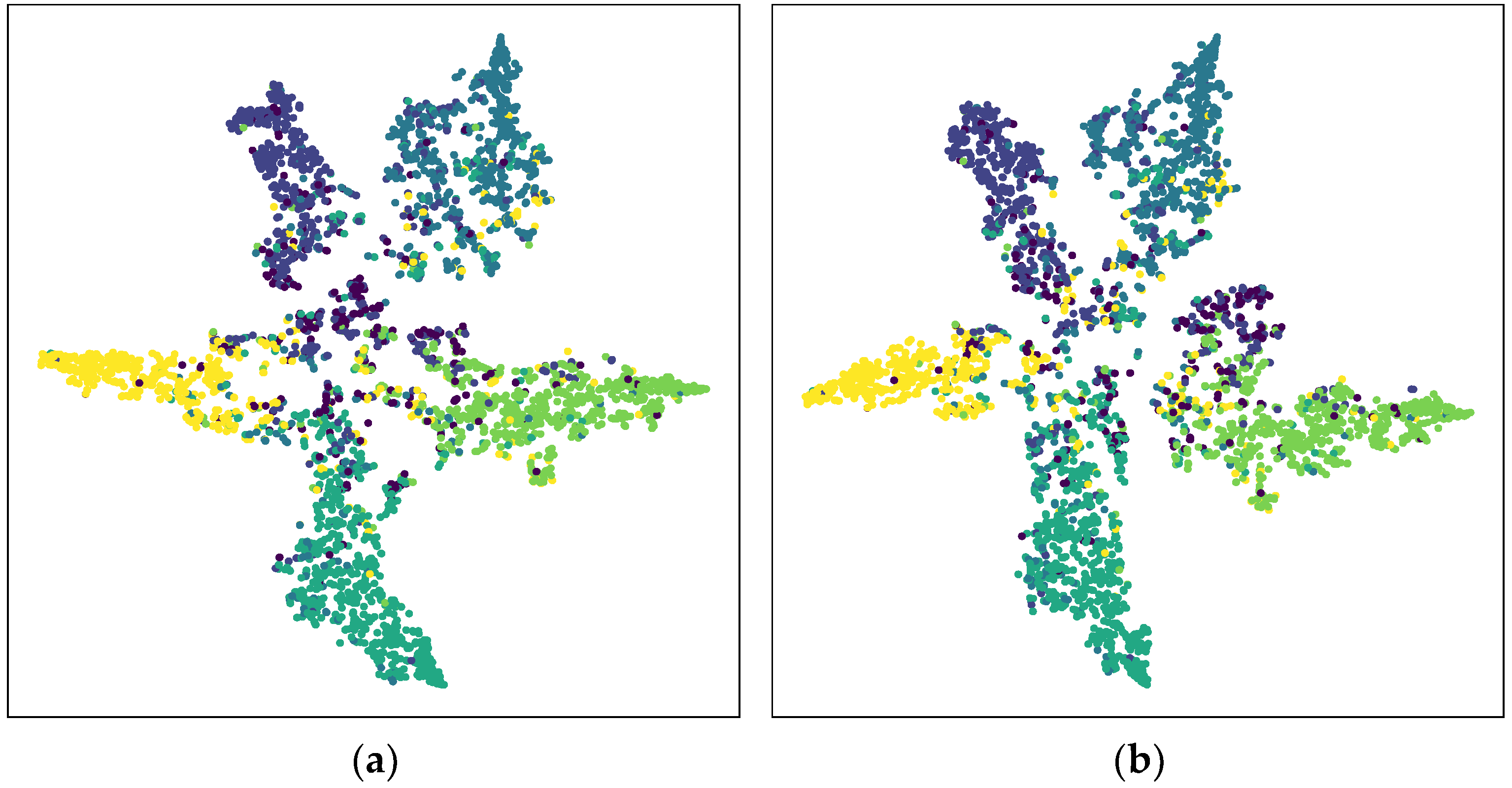
4.8. Classification Visualization

Figure 9 and Figure 10 shows the visualization of the results of the standard classification of the CiteSeer. The Figure 9a is GCN, the Figure 9b is Simple and deep graph convolutional networks (GCNII) [32], the Figure 10a is the feature extractor of PMRGNN model using the convolution layers without KL divergence, and the Figure 10b is the model proposed in this paper. It can be observed that the distribution of the Figure 9a is diffused and not clear. The Figure 9b shows that the GCNII model is more distributed than the traditional model GCN. However, according to the illustration, the node classification of GCN and GCNII is still not clear enough. The Figure 10 correspond to our model. Compared with GCNII, the node aggregation in PMRGNN is more compact, and similar nodes tend to move in one direction. In the Figure 10a, five kinds of nodes are classified obviously, and the classification of the central nodes is relatively fuzzy. In the ablation experiment of Section 4.3, we also proved that without KL divergence, the accuracy of the model will decline. We use two feature extractors to make clusters more compact and node classification clearer.

5. Conclusions

In the research of graph semi-supervised classification, this paper proposes a new model, Graph Mixed Random Network Based on PageRank (PMRGNN). Frist of all, we randomly mask the dimension with zero in the node features, and then aggregate the multi-order fields of the nodes to randomly generate new feature matrices. Secondly, we propose a method that combines two feature extractors. It enables the key information between features complement each other. Finally, we propose two losses of processing feature extractors loss and graph regularization loss to improve the performance of the model. In the experiment, we prove that our model has superior performance comparing with other neural networks. Specifically, PMRGNN is 0.3%, 2.4%, 0.2% higher than other best algorithms respectively on three data sets. Under the lower label rate, model still maintains 1.2%, 0.3% and 0.3% higher than other algorithms on three data sets. Ablation experiments show that each component of this algorithm has a corresponding role. At the same time, the component can make the verification loss close to the training loss, and make them more stable. About the selection of ${\gamma }_k$, PageRank weight has more advantages than other options. In the research of over-smoothing, with the increase of the number of layers, the accuracy of our model does not decline, and it is stable at 85%. It is proved that the algorithm can effectively alleviate the over-smoothing problem. In terms of classification visualization, PMRGNN is more intuitive than other classifications.

All in all, the idea of PMRGNN is feasible. In semi-supervised learning, the model may have a profound impact on other work. In future research, we hope to expand the strength of PMRGNN to collect effective information. At the same time, we want to improve the sampling method and enhance the scalability of proposed strategy.

References

1. Kipf, T.N.; Welling, M. Semi-supervised classification with graph convolutional networks. In Proceedings of the 5th International Conference on Learning Representations (ICLR), Toulon, France, 24–26 April 2017; pp. 1–14. [Google Scholar]
2. Abu-El-Haija, S.; Perozzi, B.; Kapoor, A.; Alipourfard, N.; Lerman, K.; Harutyunyan, H.; Steeg, G.V.; Galstyan, A. Mixhop: Higher-order graph convolutional architectures via sparsified neighborhood mixing. In Proceedings of the 36th International Conference on Machine Learning, Long Beach, CA, USA, 9–15 June 2019; pp. 21–29. [Google Scholar]
3. Rong, Y.; Huang, W.; Xu, T.; Huang, J. DropEdge: Towards Deep Graph Convolutional Networks on Node Classification. In Proceedings of the 7th International Conference on Learning Representations, New Orleans, LA, USA, 6–9 May 2019; pp. 1–18. [Google Scholar]
4. Luo, D.; Cheng, W.; Yu, W.; Zong, B.; Ni, J.; Chen, H. Learning to Drop: Robust Graph Neural Network via Topological Denoising. In Proceedings of the 14th ACM International Conference on Web Search and Data Mining, Online, 8–12 March 2021; pp. 779–787. [Google Scholar]
5. Chen, D.; Lin, Y.; Li, W.; Li, P.; Zhou, J.; Sun, X. Measuring and Relieving the Over-Smoothing Problem for Graph Neural Networks from the Topological View. In Proceedings of the 34th AAAI Conference on Artificial Intelligence, New York, NY, USA, 7 February 2020; pp. 3438–3445. [Google Scholar]
6. Zhao, T.; Liu, Y.; Neves, L.; Woodford, O.; Jiang, M.; Shah, N. Data Augmentation for Graph Neural Networks. In Proceedings of the 34th AAAI Conference on Artificial Intelligence, New York, NY, USA, 7 February 2020; pp. 1–9. [Google Scholar]
7. Klicpera, J.; Weienberger, S.; Günnemann, S. Diffusion Improves Graph Learning. In Proceedings of the 2019 Conference and Workshop on Neural Information Processing Systems, Vancouver, BC, Canada, 8–14 December 2019; pp. 1–22. [Google Scholar]
8. Xu, B.; Shen, H.; Cao, Q.; Cen, K.; Cheng, X. Graph Convolutional Networks using Heat Kernel for Semi-supervised Learning. In Proceedings of the 33th International Joint Conference on Artificial Intelligence, Macao, China, 10–16 August 2019; pp. 1–7. [Google Scholar]
9. Jiang, B.; Lin, D.; Tang, J.; Luo, B. Data Representation and Learning with Graph Diffusion-Embedding Networks. In Proceedings of the 2019 IEEE Conference on Computer Vision and Pattern Recognition, Long Beach, CA, USA, 16 June 2019; pp. 10414–10423. [Google Scholar]
10. Tsitsulin, A.; Mottin, D.; Karras, P.; Müller, E. VERSE: Versatile Graph Embeddings from Similarity Measures. In Proceedings of the 2018 World Wide Web Conference, Lyon, France, 23–27 April 2018; pp. 539–548. [Google Scholar]
11. Klicpera, J.; Bojchevski, A.; Günnemann, S. Combining Neural Networks with Personalized PageRank for Classification on Graphs. In Proceedings of the 7th International Conference on Learning Representations, New Orleans, LA, USA, 6–9 May 2019; pp. 1–14. [Google Scholar]
12. Zhu, Y.; Xu, Y.; Yu, F.; Liu, Q.; Wu, S.; Wang, L. Deep Graph Contrastive Representation Learning. In Proceedings of the 2020 International Conference on Machine Learning, Dublin, Ireland, 8–11 June 2020; pp. 1–17. [Google Scholar]
13. You, Y.; Chen, T.; Sui, Y.; Chen, T.; Wang, Z.; Shen, Y. Graph Contrastive Learning with Augmentations. In Proceedings of the 2020 Conference and Workshop on Neural Information Processing Systems, Online, 6 December 2020; pp. 5812–5823. [Google Scholar]
14. Li, J.; Zhou, P.; Xiong, C.; Hoi, S.C. Prototypical Contrastive Learning of Unsupervised Representations. In Proceedings of the 9th International Conference on Learning Representations, Online, 3–7 May 2021; pp. 1–16. [Google Scholar]
15. Kang, B.; Li, Y.; Xie, S.; Yuan, Z.; Feng, J. Exploring balanced feature spaces for representation learning. In Proceedings of the 9th International Conference on Learning Representations, Online, 3–7 May 2021; pp. 1–15. [Google Scholar]
16. Xie, Q.; Dai, Z.; Hovy, E.; Luong, T.; Le, Q. Unsupervised data augmentation for consistency training. In Proceedings of the 2020 Conference and Workshop on Neural Information Processing Systems, Online, 6 December 2020; pp. 6256–6268. [Google Scholar]
17. Xu, K.; Li, C.; Tian, Y.; Sonobe, T.; Kawarabayashi, K.; Jegelka, S. Representation Learning on Graphs with Jumping Knowledge Networks. In Proceedings of the 6th International Conference on Learning Representations, Vancouver, BC, Canada, 30 April–3 May 2018; pp. 5453–5462. [Google Scholar]
18. Wu, F.; Souza, A.; Zhang, T.; Fifty, C.; Yu, T.; Weinberger, K. Simplifying graph convolutional networks. In Proceedings of the 2019 International Conference on Machine Learning, Long Beach, CA, USA, 12 June 2019; pp. 6861–6871. [Google Scholar]
19. Zhu, H.; Koniusz, P. Simple spectral graph convolution. In Proceedings of the 9th International Conference on Learning Representations, Online, 3–7 May 2021; pp. 1–15. [Google Scholar]
20. Page, L.; Brin, S.; Motwani, R.; Winograd, T. The pagErank Citation Ranking: Bringing Order to the Web; Stanford Digital Libraries Working Paper; Stanford InfoLab: Stanford, CA, USA, 1999; pp. 1–17. Available online: http://ilpubs.stanford.edu:8090/422/1/1999-66.pdf (accessed on 1 January 2022).
21. Kondor, R.; Lafferty, J. Diffusion Kernels on Graphs and Other Discrete Structures. In Proceedings of the 2002 International Conference on Machine Learning, Sydney, Australia, 13 June 2002; pp. 315–322. [Google Scholar]
22. McPherson, M.; Smith-Lovin, L.; Cook, J. Birds of a feather: Homophily in social networks. Annu. Rev. Sociol. 2001, 27, 415–444. [Google Scholar] [CrossRef]
23. Verma, V.; Qu, M.; Kawaguchi, K.; Lemb, A.; Bengio, Y.; Kannala, J.; Tang, J. GraphMix: Improved Training of GNNs for Semi-Supervised Learning. In Proceedings of the 35th AAAI Conference on Artificial Intelligence, Online, 2 February 2021; pp. 1–21. [Google Scholar]
24. Weston, J.; Ratle, F.; Mobahi, H.; Collobert, R. Deep learning via semi-supervised embedding. Neural Netw. Tricks Trade 2012, 7700, 639–655. [Google Scholar]
25. Zhu, X.; Ghahramani, Z.; Lafferty, J.D. Semi-supervised learning using gaussian fields and harmonic functions. In Proceedings of the 20th International Conference on Machine Learning, Washington, DC, USA, 1–24 August 2003; pp. 912–919. [Google Scholar]
26. Zhu, M.; Wang, X.; Shi, C.; Ji, H.; Cui, P. Interpreting and unifying graph neural networks with an optimization framework. In Proceedings of the 30th Web Conference, Ljubljana, Slovenia, 12–23 April 2021; pp. 1215–1226. [Google Scholar]
27. Yang, H.; Ma, K.; Cheng, J. Rethinking Graph Regularization for Graph Neural Networks. In Proceedings of the 35th AAAI Conference on Artificial Intelligence, Online, 2 February 2021; pp. 4573–4581. [Google Scholar]
28. Gilmer, J.; Schoenholz, S.S.; Riley, P.F.; Vinyals, O.; Dahl, G.E. Neural message passing for quantum chemistry. In Proceedings of the the 34th International Conference on Machine Learning, Sydney, NSW, Australia, 6–11 August 2017; pp. 1263–1272. [Google Scholar]
29. Veličković, P.; Cucurull, G.; Casanova, A.; Romero, A.; Lio, P.; Bengio, Y. Graph attention networks. In Proceedings of the 6th International Conference on Learning Representations, Vancouver, BC, Canada, 30 April–3 May 2018; pp. 1–12. [Google Scholar]
30. Yang, Z.; Cohen, W.; Salakhudinov, R. Revisiting semi-supervised learning with graph embeddings. In Proceedings of the 2016 International Conference on Machine Learning, New York, NY, USA, 19–24 June 2016; pp. 40–48. [Google Scholar]
31. Chien, E.; Peng, J.; Li, P.; Milenkovic, O. Adaptive universal generalized PageRank graph neural network. In Proceedings of the 8th International Conference on Learning Representations, Addis Ababa, Ethiopia, 26 April 2020; pp. 1–24. [Google Scholar]
32. Chen, M.; Wei, Z.; Huang, Z.; Ding, B.; Li, Y. Simple and deep graph convolutional networks. In Proceedings of the 37th International Conference on Machine Learning, New Orleans, LA, USA, 13–18 July 2020; pp. 1725–1735. [Google Scholar]
33. Hamilton, W.L.; Ying, R.; Leskovec, J. Inductive representation learning on large graphs. In Proceedings of the 31st Conference on Neural Information Processing Systems, Long Beach, CA, USA, 8–14 December 2017; pp. 1025–1035. [Google Scholar]
Figure 1. Citation network and its graph structure (red is class A nodes, purple is class B nodes).
Symmetry 14 01678 g001
Figure 2. Concept of graph.
Symmetry 14 01678 g002
Figure 3. Graph convolution network under semi-supervised task.
Symmetry 14 01678 g003
Figure 4. PMRGNN model structure (red is marked nodes, purple is unmarked nodes).
Symmetry 14 01678 g004
Figure 5. Graph data augmentation.
Symmetry 14 01678 g005
Figure 6. Generalization performance on Cora (the (a) is without regularization term, the (b) is full PMRGNN model).
Symmetry 14 01678 g006aSymmetry 14 01678 g006b
Figure 7. Accuracy of different number of labels.
Symmetry 14 01678 g007
Figure 8. Over-smoothing analysis.
Symmetry 14 01678 g008
Figure 9. The t-SNE visualization of output on CiteSeer dataset. The left is GCN (a), the right is GCNII (b).
Symmetry 14 01678 g009
Figure 10. The t-SNE visualization of output on CiteSeer dataset. The left is PMRGNN without KL divergence (a), the right is full PMRGNN (b).
Symmetry 14 01678 g010