Multi-Channel Data Aggregation Scheduling Based on the Chaotic Firework Algorithm for the Battery-Free Wireless Sensor Network

Abstract

The emergence of battery-free wireless sensor networks (benefiting from the ability to collect energy from the surroundings) has broken through the energy and lifetime limitations of traditional wireless sensor network systems, but also brings challenges to the sharing of network resources. In the multi-channel wireless communication environment, in particular, how to coordinate the communication time and occupied channels of a large number of sensor nodes from the perspective of optimizing the global network has become a research problem that must be solved. To reduce the transmission delay and the usage of wireless channels, a new multi-channel data aggregation scheduling method based on the chaotic firework algorithm is proposed in this paper. With the help of the generation function of feasible solutions, one scheduling set and a firework individual can be rapidly converted to each other. By the operations of firework explosions, the Gaussian mutation, and chaotic exploration, a sub-optimal scheduling set could be found during an acceptable time period. Finally, simulation results show that the new scheduling method has advantages in aggregation delay and occupied channels when compared with existing methods.

1. Introduction

Since the energy of traditional wireless sensor nodes is limited, and it is difficult to replace the battery in many application scenarios, this directly leads to a great limitation on the life of wireless sensor networks (WSNs) [1]. The emergence of battery-free wireless sensor networks can effectively solve the above-mentioned energy limitation problem [2,3]. Battery-free sensor nodes are equipped with energy harvesting devices, which can obtain energy from the surrounding environment for power supply, such as wind energy [4], solar energy [5], radio frequency signals [6], etc., while eliminating the demand to replace batteries. The potential application fields of battery-free WSNs are very wide, such as agricultural environmental monitoring [7], natural disaster prevention [8], smart manufacturing [9], and so on, especially in the application scenarios where the batteries of sensors are not easy to replace. However, the characteristics of energy harvesting and storage also bring greater challenges to wireless communication in battery-free WSNs.

Data aggregation, as a common data processing technology in WSNs, can effectively reduce the amount of data and the number of data packets that need to be transmitted [10], and finally decrease the communication load and energy consumption. It is mainly achieved by combining data information from multiple sources into one output [11]. In addition, the application of multi-channel technology can effectively reduce communication conflicts, in which nodes just only need to switch channels under certain conditions, so that network performance can be further improved [12].

How to control the wireless communication time and achieve the goal of reducing the latency of data aggregation is an important and typical research problem in WSNs. Time Division Multiple Access (TDMA) technology is one of the most popular ways to implement the control of communication time in WSNs [13]. Inspired by the principle of TDMA, the time and channel can be viewed as scheduling resources to be allocated for sensor nodes in the multi-channel mode [14]. The communication period (or data collection period) is divided into a certain number of time slots with the exact same time lengths, where the specified nodes are permitted to perform wireless communication. The research problem of this paper involves how to efficiently allocate the respective time slot and wireless channel for each node, and construct a conflict-free multi-channel data aggregation scheduling in battery-free WSNs to maximize the network performance. The main contribution of this paper can be summarized as follows:

• Multi-channel technology was added into the data aggregation scheduling in battery-free WSNs for the first time. None of the existing data aggregation scheduling methods in WSNs considered the same network scenarios before. In this case, the scheduling task allocates both the time slot and channel for each node, rather than only the time slot.
• The problems surrounding multi-channel data aggregation scheduling for battery-free WSNs were analyzed and formulated. The optimization objective was evaluated by the fitness function, and the constraints for the feasible scheduling set were expressed in the corresponding mathematical model.
• The chaotic firework algorithm was implemented into the multi-channel data aggregation scheduling method for battery-free WSNs. Scheduling sets are represented by the firework individuals; the firework population continuously evolves to discover better solutions. A chaotic map function was integrated into the solution optimization process, thereby enhancing the global search capability.

The employment of Internet of Things (IoT) technology is an essential part of Agriculture 4.0, where sensors replace the human monitoring of the objective and environment [15,16]. This characteristic makes Agriculture 4.0 one of the most possible application fields in the proposed scheduling method. The existing research studies on Agriculture 4.0 have focused on the application of energy harvesting technology in recent years [17,18], such as using solar energy [19], but the problem of how to realize conflict-free wireless communication with low transmission latency has not been adequately discussed until now. However, with the help of the proposed scheduling method, WSNs can simultaneously utilize energy harvesting and multi-channel technology without considering communication conflict problems, thereby the capability of the Agriculture 4.0 system is enhanced, and more application scenarios could be supported.

The rest of the paper is organized as follows: Section 2 discusses the existing research studies related to the topic of this paper. Section 3 introduces the target system model and illustrates the problem to be solved. Section 4 illustrates the principle and components of the proposed multi-channel data aggregation scheduling method. Section 5 presents the theoretical analysis for the complexity and the convergence of the proposed method. Section 6 presents the simulation platform and analyzes the simulation result in order to prove the performance advantages of the proposed method. Finally, Section 7 concludes the current works.

2. Related Works

The vast majority of existing research studies on data aggregation scheduling focus on traditional WSNs with a single wireless channel [13,20]. Few researchers pay attention to the multi-channel mode and battery-free sensor nodes. Until now, none of these research studies have put both conditions into the network environment for data aggregation scheduling.

Multi-channel TDMA scheduling algorithms—aimed at minimizing the total energy consumption in a network—were proposed by S. Kumar et al. [21]. Multiple RF channels were utilized to alleviate collisions and support concurrent communications in this work. Even though only sub-optimal schedules for data gathering could be obtained, this heuristic algorithm offers computationally efficient scheduling operations. Bagaa et al. developed a cross-layer trusted data aggregation scheduling method for multi-channel WSN [22]. K-disjoint paths were constructed for each source node to the sink node according to the aggregation tree in this method (a conflict-free communication schedule could then be generated). Jiao et al. utilized the candidate activity conflict and feasible activity conflict graph to describe the node scheduling relationship [23], and proposed the graph coloring method to achieve efficient scheduling. Ren M. et al. proposed a cluster-based distributed data aggregation scheduling algorithm with multi-power and multi-channels [24], where the network nodes were put into multiple clusters; different power levels were used for inner cluster communications and the communications among cluster heads separately. A conflict-free TDMA link scheduling method [25] was proposed by Lee et al. to minimize the time slot lengths of multi-channel wireless multi-hop wireless sensor networks, where the min–max method is used to optimize the time slot length, and the sorting algorithm is used to minimize the end-to-end delay.

T. Zhu et al. proposed a data aggregation scheduling method in battery-free WSNs [26]; the minimum latency aggregation scheduling (MLAS) problem in battery-free WSNs were investigated and proved as non-deterministic polynomial (NP)-hard; they finally constructed the scheduling set according to an aggregation tree. The distributed energy-adaptive aggregation scheduling method with a coverage guarantee was proposed by K. Chen et al. [27] for battery-free WSNs. This algorithm selects the nodes adaptively according to their energy conditions and then allocates time slots for the selected nodes to achieve the minimum latency. The structure-free general data aggregation scheduling method proposed by Q. Chen et al. [28] involves the computation of a conflict-free schedule simultaneously, relying on non-predetermined structures. Two latency and energy-efficient algorithms were developed for both the single query and the multiple-query MLAS problem.

Y. Cai et al. applied the chaotic fireworks algorithm to solve the TSP problem [29], where the logistic map function was utilized to generate a chaotic sequence to improve the search capability in the discrete solution space. In [30], Luo W. et al. used two hybrid chaotic systems to generate more uniform fireworks, meanwhile, they developed a new chaotic perturbation operator to accelerate the algorithm convergence and help the algorithm jump out of the local optimum.

In general, there is no existing work on the research data aggregation scheduling method for battery-free WSNs with multi-channel modes—until now. The chaotic firework algorithm is a feasible option to realize the scheduling method in battery-free WSNs.

3. System Model and Problem Statement

3.1. System Model

A battery-free WSN can be abstracted as a graph $G\left(V,\overrightarrow{L}\right)$ where V and $\overrightarrow{L}$ denote the set of sensor nodes and the set of communication links (edges), respectively. Sensor nodes use a half-duplex transmission mode, where one node cannot perform data transmission and data reception at the same time. The symmetric communication environment was adopted in this paper, where if any pair of the nodes $v_i\in V$ and $v_j\in V$ is located within the wireless communication range of each other, both links ${\overrightarrow{l}}_{i,j}$ and ${\overrightarrow{l}}_{j,i}$ exist in the network. To achieve further symmetry, each node has the same data transmission rate and data reception rate. In addition, the communication radius $r_{com}$ and the interference radius $r_{int}$ of one sensor node are the same. An example of symmetric communication is depicted in Figure 1. The nodes located in the wireless communication range of $v_i$ are called neighbors $ngh\left(v_i\right)$. In a data collection period, sensing data are generated on source nodes $v_{src}$ and are supposed to be transmitted to a unique destination, which is called the sink node S. Data packets are delivered from sources to the sink. Intermediate nodes between source and sink nodes perform data aggregation and forward the processed result. The set of available wireless channels is represented by C; $c_k\in C$ denotes the $k_{th}$ channel.

The data collection period is defined as a frame $T_c$ that consists of a fixed number of time slots. In each time slot, the links without communication conflict and sufficient energy could be concurrently scheduled to perform wireless communication. The time slot sets (of reception and transmission) are respectively denoted by $T_{rx}$ and $T_{tx}$. The battery-free sensor node is able to absorb energy from the surrounding environment. To facilitate modeling, the charging rate $e^{chr}\left(t\right)$ of a node for timestep t was predictable in our research. Meanwhile, the unit of energy is expressed in percent, the energy capacity is $e^{cap}$ for one node, $e^{ini}$ denotes the initial energy level, and the energy consumption for time transmission and reception is represented by $e^{rx}$ and $e^{tx}$. Based on the above definitions, the residual energy level $e_i^{rsd}$ of a node $v_i$ can be predicted at the end of one time slot t, and it can be expressed as follows:

$$e_i^{rsd}\left(t\right)=\left\{\begin{array}{c}min(e_i^{rsd}(t-1)+e_i^{chr}\left(t\right)-e^{rx},e^{cap}),t\in T_{rx}\hfill \\ min(e_i^{rsd}(t-1)+e_i^{chr}\left(t\right)-e^{tx},e^{cap}),t\in T_{tx}\hfill \\ min(e_i^{rsd}(t-1)+e_i^{chr}\left(t\right),e^{cap}),otherwise\hfill \end{array}\right.$$

(1)

In Figure 2, an example of the energy level change on the sensor node can be found, where $e^{ini}=0,e^{tx}=40,e^{rx}=30$, and the charging rate is set as a constant $e^{chr}=20$. At the beginning of a frame, the current node with empty residual energy starts to harvest energy. In $T_{rx}$, two reception operations occur and energy levels are slightly reduced to 20. After $T_{tx}$, the current node harvests energy until reaching its capacity.

The routing protocol is not the focus of this research. By adopting a typical data aggregation routing method in [31], the routing structure toward many-to-one communication can be constructed before communication scheduling. Due to the operation of data aggregation, multiple data packets from the upstream nodes $Up\left(v_i\right)$ are combined as one outgoing data packet on any node $v_i$, and this packet will be transmitted to the downstream node $Dn\left(v_i\right)$.

3.2. Problem Statement

The fundamental task of the multi-channel data aggregation scheduling method for battery-free WSNs involves allocating the time slot and wireless channel for each node without communication conflict and energy insufficiency in order to maximize the network performance. According to the adopted system model, if the allocation of the time slot and channel are unreasonable, two types of communication conflicts and one type of energy insufficiency possibly appear in the network. When the terminal is denoted as the reception or transmission node of any communication links, these situations can be described as follows:

• Direct communication conflict: When two or more links that possess at least one exact same terminal are allocated for the same time slot, then this overlapping terminal has a communication conflict. One node cannot concurrently handle two or more communication tasks at the same time slot. $C{C}_{dt}({\overrightarrow{l}}_{i,j})$ denotes the set of the links with the direct communication conflict for ${\overrightarrow{l}}_{i,j}$; this set can be obtained after constructing the routing structure.
• Indirect communication conflict: When the receiving terminal of one link is located in the interfering range of the transmitting terminal of another link, and both links are allocated the same time slot and channel, then the indirect communication conflict appears. $C{C}_{id}({\overrightarrow{l}}_{i,j})$ denotes the set of links with indirect communication conflict for ${\overrightarrow{l}}_{i,j}$; this set can be obtained after constructing a routing structure as well.
• Energy insufficiency: When the residual energy level of any node $e_i^{rsd}$ drops below 0 percent, this node is assumed to be no longer functional; no operation can be executed on this node anymore.

An example of direct and indirect communication conflicts is depicted in Figure 3, where the solid lines denote that the links belong to $RS$, and the dotted lines denote the links that do not belong to $RS$. In a direct communication conflict, $v_5$ cannot receive data packets from $v_2$ and $v_3$ in the same time slot $t_3$. Even though different channels are adopted, one node can only receive one packet per time slot. In the indirect communication conflict, $v_5$ is located in the interfering range of $v_1$, when ${\overrightarrow{l}}_{1,4}$ is performed in $t_3$ and $c_1$, $v_5$ cannot successfully receive the data packet from $v_2$.

From the viewpoint of a global network, multi-channel data aggregation scheduling involves a set of three-tuple; each three-tuple contains the information of the time slot and channel for one link in the routing structure $RS$. A scheduling set can be expressed as $DS=\{\cdots ,{\overrightarrow{ds}}_{i,j},\cdots \}$, where the length of the frame is $\left|DS\right|$ and equal to $\left|RS\right|$. ${\overrightarrow{ds}}_{i,j}=({\overrightarrow{l}}_{i,j},t^{i,j},c^{i,j})$ denotes the allocated time slot $t^{i,j}$ and channel $c^{i,j}$ for the link ${\overrightarrow{l}}_{i,j}$; an example can be found in Figure 4, where $d{s}_{1,4}=({\overrightarrow{l}}_{1,4},t_3,c_1)$, $t^{1,4}=t{s}_3$ and $c^{1,4}=c{h}_1$.

Time and channel are considered the most important resources of wireless communication in this paper. Since both resources are limited in a realistic environment, the overall optimization objective of multi-channel data aggregation scheduling is to minimize their occupations. Even so, the optimization objectives can be alternated according to the specific application demand. Let $v_t$ and $v_c$ represent the objective functions of the time slot and channel, the scheduling problem is expressed as $\underset{DS}{argmin}\left\{f(v_t\left(DS\right),v_c\left(DS\right))\right\}$, where f denotes the fitness function, and the solution should be subject to the following constraints:

• $(DS-d{s}_{i,j})\cap d{s}_{i,j}=⌀,\forall {\overrightarrow{l}}_{i,j}\in RS$
• If ${\overrightarrow{l}}_{i,j}\in RS$, $\forall {\overrightarrow{l}}_{i,m}\in RS$ or ${\overrightarrow{l}}_{n,j}\in RS$, then $d{s}_{i,m}·t^{i,m}\ne d{s}_{i,j}·t^{i,j}$ or $d{s}_{n,j}·t^{n,j}\ne d{s}_{i,j}·t^{i,j}$
• If ${\overrightarrow{l}}_{i,j}\in RS$, $\forall d{s}_{i,m}\in \overrightarrow{L}$ and $\notin RS$, ${\overrightarrow{l}}_{n,m}\in \overrightarrow{L}$, then $d{s}_{i,j}·t^{i,j}\ne d{s}_{n,m}·t^{n,m}$ or $d{s}_{i,j}·c^{i,j}\ne d{s}_{n,m}·c^{n,m}$
• $T_{rx}\left(v_i\right).end<T_{tx}\left(v_i\right),\forall v_i\in V$
• $T_{tx}\left(Up\left(v_i\right)\right)<T_{tx}\left(v_i\right)<T_{tx}\left(Dn\left(v_i\right)\right),\forall v_i\in V$
• $\forall t\in T_{rx}$, $\exists e_i^{rsd}(t-1)\ge e^{rx}$
• $\forall t\in T_{tx}$, $\exists e_i^{rsd}(t-1)\ge e^{tx}$

The first constraint is that the communication on each link can only be performed once, so the allocation of the slot and channel $d{s}_{i,j}$ for a link ${\overrightarrow{l}}_{i,j}$ is unique. The second constraint indicates the avoidance of direct communication interference, when a certain link ${\overrightarrow{l}}_{i,j}$ performs communication, then any link with the overlapping terminals cannot perform communication at the same time slot. The third constraint indicates the avoidance of indirect communication interference; the links with interference cannot occupy the same time slot or the same channel. The fourth constraint is generated from the principle of data aggregation, where an aggregated result is supposed to be transmitted after receiving all expected data from upstream nodes. The fifth constraint explains that the transmission operation of the current node should locate between its downstream node and its upstream node. The last two constraints denote that the residual energy levels have to be larger than the required amount for wireless reception or transmission.

The essence of the scheduling problem is to find the best allocation set of time slots and channels for links that satisfy the optimization goals and constraints. An example of multi-channel data aggregation scheduling for battery-free WSNs can be found in Figure 4. The routing structure is expressed as $RS=\{{\overrightarrow{l}}_{1,4},{\overrightarrow{l}}_{2,5},{\overrightarrow{l}}_{3,5},{\overrightarrow{l}}_{4,S},{\overrightarrow{l}}_{5,S}\}$. A feasible solution is successfully constructed by avoiding communication conflicts and energy insufficiency; this solution allocates the time slots and channels for each link, respectively. This scheduling is expressed as $DS=\{({\overrightarrow{l}}_{1,4},t_3,c_1),({\overrightarrow{l}}_{2,5},t_3,c_2),({\overrightarrow{l}}_{3,5},t_4,c_2),({\overrightarrow{l}}_{4,S},t_4,c_1),({\overrightarrow{l}}_{5,S},t_6,c_1)\}$, each three-tuple corresponds to a link of $RS$ in order, for example, $d{s}_{1,4}=({\overrightarrow{l}}_{1,4},t_3,c_1)$.

Theorem 1.

Multi-channel data aggregation scheduling for battery-free WSNs (MDSB) is a NP-hard problem.

Proof. 

Let the number of available channels be 1 $\left|C\right|=1$, then the network becomes the traditional single-channel network. Let the charging rate of each battery-free sensor be 0, where $e_i^{chr}=0,\forall v_i\in V$. Meanwhile, let the energy capacity $e_i^{cap},\forall v_i\in V$ of each battery-free sensor be the battery capacity of traditional battery-powered WSNs, and set the initial energy level to the full energy capacity $e_i^{ini}=e_i^{cap}$. In this case, the MDSB problem transforms to the minimum latency aggregation scheduling (MLAS) problem in WSNs, and the latter problem becomes a special case of the former problem. The MLAS problem has already been proved as NP-hard in the existing research [32,33]; therefore, MDSB is also NP-hard.    □

4. Scheduling Method Based on the Chaotic Firework Algorithm

The theory of the firework algorithm comes from the explosion phenomenon of fireworks [34]. Each firework individual is regarded as a feasible solution in the solution space. Then the process of generating a certain number of sparks in the firework explosion is actually the process of the neighborhood search for a feasible solution. By filtering the firework and spark with poor quality in multiple iterations, the optimal solution to the set problem can be discovered quickly. The explosion radius and the number of explosion sparks of each firework are different. The firework with poor fitness value has a larger explosion radius, which makes it have global search ability. Correspondingly, the firework with a good fitness value has a small explosion radius, which makes it have local search ability. Fireworks perform resource allocation and information exchange according to their fitness values so that the entire population can achieve a balance between the global search ability and local search ability [35]. The chaotic fireworks algorithm implants chaotic sequences into the original version, which further improves the search ability of the algorithm [30]. The chaotic fireworks algorithm consists of five parts: firework encoding, explosion detection, Gaussian mutation, chaotic replacement, and selection strategy.

4.1. Firework Encoding

To directly encode the scheduling set, $DS$ as a firework individual cannot ensure its feasibility during the process of explosion detection, Gaussian mutation, and chaotic replacement, because these evolution operations have different levels of randomness. The newly generated scheduling set has a high probability of violating the defined constraints for the MDSB problem; therefore, it is not a feasible solution. To avoid generating meaningless solutions, the priority set is applied as the encoding scheme for the firework individual.

Any link ${\overrightarrow{l}}_{i,j}$ in the routing structure $RS$ is assigned a priority (weight) $w_{i,j}$ within the range of $\{w^{min},w^{max}\}$. Then a routing structure $RS$ corresponds to a priority set $WS$, which can be used as input for the function of generating a feasible solution $\phi \left(WS\right)$. The generation of the scheduling set is based on the iteration of the timestep. At each timestep, the links in the ready state are possibly added to the scheduling set according to priority and communication conflicts. Assume the completed scheduling set as $DS\left(t\right)$ at timestep t, where the corresponding links in $DS\left(t\right)$ have already been allocated to the time slot and channel. Then the definition of the ready state of any link ${\overrightarrow{l}}_{i,j}$ is expressed as follows:

• $\forall v_k\in Up\left(v_i\right)$ and ${\overrightarrow{l}}_{k,i}\in RS,\exists d{s}_{k,i}\in DS\left(t\right)$
• $e_i^{rsd}(t-1)\ge e^{tx}$
• $e_j^{rsd}(t-1)\ge e^{rx}$

The detailed procedure is described in Algorithm 1. If the scheduling task is not complete for all links in $RS$, the generating iteration continues. In each timestep t, the current candidate link set $CL\left(t\right)$ and the set of links in the ready state $RD\left(t\right)$ are initialized first. In lines 4–8, we find all links in the ready state and put them into $RD\left(t\right)$. After sorting $RD\left(t\right)$ into $R{D}_s\left(t\right)$, the algorithm circularly detects each link ${\overrightarrow{l}}_{i,j}$ in $R{D}_s\left(t\right)$ according to its priority. In lines 10–20, the links with communication conflicts are handled appropriately. If there is a direct communication conflict, we stop scheduling the current link and jump to the next. If there is an indirect communication conflict, and the available channel is not empty, then a new channel is allocated to the current link. In lines 21–22, the scheduling tuple is complete for ${\overrightarrow{l}}_{i,j}$, and update $DS\left(t\right)$ and $CL\left(t\right)$. Once the allocation of the current timestep is complete, then the priority set removes $CL\left(t\right)$ and moves to the next timestep in lines 24–25. An example of the function to generate a feasible solution is depicted in Figure 5. The priority is set among $\{0,1\}$ in this case, and after generation, a feasible scheduling set $DS=\{({\overrightarrow{l}}_{1,4},t_3,c_1),({\overrightarrow{l}}_{2,5},t_3,c_2),({\overrightarrow{l}}_{3,5},t_4,c_1),({\overrightarrow{l}}_{5,S},t_6,c_1),({\overrightarrow{l}}_{4,S},t_7,c_1)\}$ is obtained as the output of Algorithm 1.

Algorithm 1 Function of generating a feasible solution

1: $t=1,DS\left(t\right)=⌀$; 2: while $\left|DS\left(t\right)\right|<\left|RS\right|$ do 3:    $CL\left(t\right),RD\left(t\right)=⌀$; 4:    for ${\overrightarrow{l}}_{i,j}$ in $WS$.link do 5:      if ${\overrightarrow{l}}_{i,j}$.state == ready then 6:         $RD\left(t\right)=RD\left(t\right)\cup {\overrightarrow{l}}_{i,j}$ 7:      end if 8:    end for 9:    $R{D}_s\left(t\right)=RD\left(t\right).sort\left(\right)$; 10:    for ${\overrightarrow{l}}_{i,j}$ in $R{D}_s\left(t\right)$ do 11:      if $C{C}_{dt}({\overrightarrow{l}}_{i,j})\cap CL\left(t\right)\ne ⌀$ then 12:         continue; 13:      end if 14:      if $C{C}_{id}({\overrightarrow{l}}_{i,j})\cap CL\left(t\right)\ne ⌀$ then 15:         if $c<c_{max}$ then 16:           c++; 17:         else 18:           continue; 19:         end if 20:      end if 21:      $d{s}_{i,j}=({\overrightarrow{l}}_{i,j},t,c),DS\left(t\right)=DS\left(t\right)\cup d{s}_{i,j}$; 22:      $CL\left(t\right)=CL\left(t\right)\cup {\overrightarrow{l}}_{i,j}$; 23:    end for 24:    $WS$.remove($CL\left(t\right)$); 25:    t++; 26: end while

4.2. Explosion Detection

The primary task of explosion detection is to search the sparks with better quality in the vicinity of the original fireworks. Fireworks with better quality generate more sparks in a smaller range of their neighborhoods, while fireworks with poor quality produce fewer sparks in a larger range of their neighborhoods. The firework or spark quality is represented by the fitness value. Assume that the algorithm has N initial fireworks for solving the problem. The number of explosion sparks $M_i$ and the radius $R_i$ of the explosion for one firework $W{S}_i$ can be calculated by the following equations:

$$M_i=M_{def}·\frac{f_{max}-f_i+ϵ}{{\sum }_{i=1}^N(f_{max}-f_i+ϵ)}$$

(2)

$$R_i=R_{def}·\frac{f_i-f_{min}+ϵ}{{\sum }_{i=1}^N(f_i-f_{min}+ϵ)}$$

(3)

In Equations (2) and (3), $M_{def}$ and $R_{def}$, respectively, denote the default spark number and explosion radius. $f_i$ is the fitness value for the firework $W{S}_i$, meanwhile, $f^{max}$ and $f^{min}$ are the maximum and minimum fitness values in the current firework population. $ϵ$ is the machine minimum value that is used to avoid the division by zero. In order to further ensure that the spark number of high-quality fireworks is not too much, and the spark number of low-quality fireworks is not too small, the number of sparks should be controlled within the range of $M_{min},M_{max}$, where $M_{min}$ and $M_{max}$ are the predefined maximum and minimum number of sparks.

$$M_i=\left\{\begin{array}{c}{M}_{min},M_i<M_{min}\in T_{rx}\hfill \\ M_i,M_{min}\ge M_i\ge M_{max}\hfill \\ M_{max},M_i>M_{max}\hfill \end{array}\right.$$

(4)

When the explosion occurs, the firework $W{S}_i$ randomly selects a certain number of dimensions for the position offset, thereby generating new sparks. The position update equation for the dimension k is expressed as follows:

$$w_k^i=w_k^i+R_i·U(-1,1)$$

(5)

where $w_k^i$ is the priority of the $k^{th}$ dimension of the firework $W{S}_i$, and $U(-1,1)$ denotes uniform distribution.

4.3. Gaussian Mutation

Gaussian mutation has the effect of increasing the diversity of firework populations. This mutation randomly selects a certain number of fireworks and dimensions for each firework to perform the Gaussian mutation operation. To perform a Gaussian mutation operation on a dimension k of fireworks, $W{S}_i$ can be expressed as:

$$w_k^i=w_k^i·N(1,1)$$

(6)

where $N(1,1)$ represents a Gaussian distribution with a mean of 1 and a variance of 1.

4.4. Chaotic Replacement

Chaos is a non-periodic phenomenon peculiar to nonlinear systems [36]. The ergodicity and randomness of the chaotic search are beneficial to enhancing the global search ability of the firework algorithm and to jumping out of the local optimal solution in the search process [37]. The chaos replacement is used in the application of the firework algorithm.

The main task is to firstly find the firework individuals whose fitness value is in the bottom $\sigma$ percentage of the current firework population $FS$ and to generate a candidate replacement set. Subsequently, the algorithm generates the same number of the chaotic sequences with the replacement set through chaotic ergodic search and converts the chaotic sequences into firework individuals in the solution space. A replacement occurs only if the quality of the new solution is better than any individual in the current replacement set. Finally, for the candidate set of firework individuals, $F{S}_i$, $Q_i$ denotes the real number of individuals replaced by new chaotic sequences.

The discrete memristor-based model, compared with the original chaotic map functions, has a memory effect and stronger nonlinearity; these features can make the map function obtain a better chaotic effect and further improve the ergodicity and randomness. The discrete memristor-based Hénon map [38] was adopted to generate a firework individual $W{S}_i$ in this research and the corresponding three-dimensional map equations are described in Equation (7). In these equations, $x_{st}$ is the generated chaotic number at the cumulative step $st$; $a,b$ are the system parameters.

$$\left\{\begin{array}{c}{x}_{st}=1+(R_1-R_2·z_{st-1})·y_{st}-a·x_{st-1}^2\hfill \\ y_{st}=b·x_{st-1}\hfill \\ z_{st}=z_{st-1}+k·y_{st}\hfill \end{array}\right.$$

(7)

where $z_0=q_0+k·y_0$, when $n>l,z_{n+1}$ changes to $z_{n+1}=z_n+k·(y_{n+1}-y_{n-l})$. The memory of this discrete memristor is defined to the past l states, and l is set as 100 in this paper.

$$q_{st}=\left\{\begin{array}{c}mod(x_{st},1),if{x}_{st}>1\hfill \\ mod(x_{st},-1),if{x}_{st}<-1\hfill \end{array}\right.$$

(8)

Equation (8) ensures the generated value of this mapping function is located among the range of $[-1,1]$. If the value ranges of the firework individual and chaotic sequence are the same, then $q_{st}$ is directly equal to the individual $w{s}_i$. Otherwise, the chaotic sequence should convert to the individual by the following function:

$$w_k^i=0.5·q_{st}·(w_{max}-w_{min})+w_{mean}$$

(9)

where the chaotic number $q_{st}$ can convert to the $k^{th}$ dimension of the priority $w_k^i$ of a firework individual. In addition to the chaotic replacement, the chaotic sequence is exploited to initialize the firework individuals at the beginning of the scheduling method as well.

4.5. Selection Strategy

The original fireworks, explosion sparks, and Gaussian mutation jointly generate the candidate set $FS$ of the firework population, and chaotic replacement updates this set. From this set, N firework individuals should be selected as the next generation of firework population. The individual with the current optimal fitness value is retained unconditionally, and on this basis, the remaining $N-1$ firework individuals are selected according to the roulette rules. The probability that each firework in the set k is selected is:

$$p_i=\frac{{\sum }_{j=1}^{\left|FS\right|}{d}_{ij}}{{\sum }_{i=1}^{\left|FS\right|}{\sum }_{j=1}^{\left|FS\right|}{d}_{ij}}$$

(10)

$$d_{ij}=|w^i-w^j|$$

(11)

where $d_{ij}$ is the euclidean distance between two firework individuals. Under the action of Equation (3), the deviation of an individual from other individuals is larger; consequently, its selection probability is higher as well. This mechanism avoids the selection probability of the group in dense locations being too large, potentially falling into a local optimum, but it does not necessarily guide the group to evolve in a good direction.

4.6. Description of Scheduling Procedure

At the beginning of scheduling, N firework individuals are initialized by a chaotic search and put into the set $WS$. When the iteration of the chaotic firework algorithm starts, the primary task is to construct the candidate firework set $FS$ for the next round of evolution in lines 4–8. In this process, a firework individual converts to a feasible solution $x_i$ through Algorithm 1. In lines 6–7, explosion detection and Gaussian mutation are performed on $x_i$, and then construct the current firework set $F{S}_i$. Chaotic exploration attempts to optimize further the individuals in $F{S}_i$ by a chaotic search. The best N individuals in $FS$ are selected as $WS$ in line 11. Through the continuous iteration of the above steps, the solutions with better quality will be found, and finally, converge to an approximate optimal solution.

5. Theoretical Analysis

5.1. Complexity Analysis

As a scheduling algorithm based on centralized computing, the proposed method targets the searching for a sub-optimal solution inside an acceptable time period without occupying too much memory space. For the function of generating a feasible solution in Algorithm 1, the construction of each involving data structure is based on the routing structure $RS$, so the space complexity of this part can be expressed as $O\left(\left|RS\right|\right)$. The time complexity of the outer while loop can be expressed as $O\left(\left|RS\right|\right)$. As for the inner while loop, the set construction of the links in the ready state costs $O\left(\left|RS\right|\right)$ time complexity as well. The time complexity of the sorting operation is denoted as $O(\left|RS\right|+\left|RS\right|·\log \left|RS\right|)$, and the time complexity of handling the links with conflicts is denoted as $O\left(\left|RS\right|\right)$. In this case, the time complexity $O_{fs}$ of this function can be expressed as follows:

$$\begin{array}{cc}\hfill O_{fs}& =O(\left|RS\right|·(\left|RS\right|+\left|RS\right|·\log \left|RS\right|+\left|RS\right|))\hfill \\ \hfill & =O({\left|RS\right|}^2·\log \left|RS\right|)\hfill \end{array}$$

(12)

For the scheduling process in Algorithm 2, the space complexity involving the data structure can be described as $O(\left|FS\right|·\left|RS\right|)$, which is affected by both the current firework population $FS$ and the routing structure $RS$. The time complexity of initializing the firework population is $O\left(N\right)$, and the iteration loop cost $O\left(It\right)$. For each firework individual, it has to be converted to a feasible solution at first and the time complexity is $O({\left|RS\right|}^2·\log \left|RS\right|)$, according to Equation (11). The operations of explosion detection, Gaussian mutation, and chaotic replacement cost $O\left(M_{max}\right)$ complexity at most. The selection strategy for the next generation of the firework population has the time complexity of $O(N·M_{max})$. Finally, the time complexity $O_{ds}$ of the entire scheduling method based on the chaotic firework algorithm can be expressed as follows:

Algorithm 2 Procedure of multi-channel data aggregation scheduling

1: Initialize N firework individuals as $WS$; 2: while iteration condition is not met do 3:    for each $W{S}_i\in WS$ do 4:      $x_i.DS=\phi \left(W{S}_i\right)$; 5:      $x_i.fitness=f(x_i.DS)$; 6:      $F{S}_i=explosion(x_i,M_i,R_i)$; based on Equations (2)–(5); 7:      $F{S}_i=mutation\left(F{S}_i\right)$ based on Equation (6); 8:      $F{S}_i=replacement(F{S}_i,\sigma )$ based on Equations (7) and (8); 9:      $FS=FS\cup F{S}_i$ 10:    end for 11:    $WS=select(FS,N)$ based on Equations (9)–(10); 12: end while

$$\begin{array}{cc}\hfill O_{ds}=& O(N+It·(N·({\left|RS\right|}^2·\log \left|RS\right|\hfill \\ \hfill & +M_{max})+N·M_{max}))\hfill \\ \hfill =& O(It·(N·({\left|RS\right|}^2·\log \left|RS\right|+M_{max})))\hfill \end{array}$$

(13)

5.2. Convergence Verification

The convergence feature of the original firework algorithm has already been studied from a theoretical level in [39]. Based on the model and conclusion of this study, the convergence feature of our scheduling method can be verified as well.

Definition 1.

The stochastic process of the chaotic firework algorithm is denoted as ${\left\{\psi \left(t\right)\right\}}_{t=0}^{\infty }$, where ${\left\{\psi \left(t\right)\right\}}_{t=0}^{\infty }=\{WS\left(t\right),M\left(t\right),R\left(t\right),Q\left(t\right)\}$, and $WS\left(t\right)=\{W{S}_1,\cdots ,W{S}_N\}$ denote the firework population at iteration t, $M\left(t\right)=\{M_1,\cdots ,M_N\}$ and $R\left(t\right)=\{R_1,\cdots ,R_N\}$ denote the explosion number and radius, respectively; finally, $Q\left(t\right)=\{Q_1,\cdots Q_N\}$ represents the number of new individuals generated by the chaotic exploration.

Definition 2.

The optimal area of the fitness function $f\left(\phi \right(WS\left)\right)$ is denoted as $R_{opt}=\{y\in WS\left|f\left(y\right)-f\left(y^{*}\right)<ϵ,ϵ>0\right\}$, where y and $y^{*}$ denote a solution and an optimal solution, respectively.

Definition 3.

The optimal state of the chaotic firework algorithm is expressed as ${\psi }^{*}\left(t\right)=\{W{S}^{*}\left(t\right),$$M\left(t\right),R\left(t\right),Q\left(t\right)\}$, if $W{S}_i\left(t\right)\in R_{opt}$ then $W{S}_i\left(t\right)\in W{S}^{*}\left(t\right)$. It means that the firework individual in ${\psi }^{*}\left(t\right)$ locates in the optimal area $R_{opt}$.

Definition 4.

The state space of the chaotic firework algorithm is represented as Ψ, and the optimal state space is represented as ${\Psi }^{*}$, where there is an optimal solution $y^{*}\in W{S}^{*}$ and $y^{*}\in R_{opt}$ for any state ${\psi }^{*}\left(t\right)=\{W{S}^{*}\left(t\right),M\left(t\right),R\left(t\right),Q\left(t\right)\}\in Psi$.

Lemma 1.

${\left\{\psi \left(t\right)\right\}}_{t=0}^{\infty }$ is an absorbing Markov stochastic process.

Proof. 

The state $\psi \left(t\right)=\left\{WS\right(t),M(t),R(t),Q(t\left)\right\}$ depends on $\left\{WS\right(t-1),M(t-1),R(t-1),Q(t-1\left)\right\}$, and the probability $P\{\psi \left(t\right)\left|\psi \left(1\right),\psi \left(2\right),\cdots \psi (t-1)\right\}=P\{\psi \left(t\right)\left|\psi (t-1)\right\}$, then ${\left\{\psi \left(t\right)\right\}}_{t=0}^{\infty }$ is a Markov stochastic process. If a solution $W{S}^k\left(t\right)\in WS\left(t\right)$ locates in the optimal area of $R_{opt}$, and the state $\psi \left(t\right)$ also stays in the optimal state space ${\Psi }^{*}$. The reason is that $W{S}^k\left(t\right)$ is the best location for all fireworks, according to the selection strategy, the solution $W{S}^k(t+1)$ for the timestep $t+1$ will be no worse than $W{S}^k\left(t\right)$, and the state $\psi (t+1)$ belongs to the optimal state space $\Psi$ as well. In this case, $P\{\psi \left(t\right)\notin \Psi \left|\psi (t-1)\in \Psi \right\}=0$; therefore, ${\left\{\psi \left(t\right)\right\}}_{t=0}^{\infty }$ is an absorbing Markov stochastic process. □

Definition 5.

For an absorbing Markov process ${\left\{\psi \left(t\right)\right\}}_{t=0}^{\infty }=\{WS\left(t\right),M\left(t\right),R\left(t\right),Q\left(t\right)\}$ and an optimal state space ${\Psi }^{*}$, if $\lambda \left(t\right)=P\psi \left(t\right)\in {\Psi }^{*}$ represents the probability that the stochastic state arrives at the optimal state at timestep t, and then ${lim}_{t\to \infty }\lambda \left(t\right)=1$ or ${lim}_{t\to \infty }P\psi \left(t\right)\in {\Psi }^{*}=1$, then ${\left\{\psi \left(t\right)\right\}}_{t=0}^{\infty }$ is called the convergence of the chaotic firework algorithm.

Theorem 2.

For an absorbing Markov process ${\left\{\psi \left(t\right)\right\}}_{t=0}^{\infty }=\{WS\left(t\right),M\left(t\right),R\left(t\right),Q\left(t\right)\}$ of the chaotic firework algorithm and an optimal state space ${\Psi }^{*}$, if $P\{\psi \left(t\right)\in {\Psi }^{*}\left|\psi (t-1)\notin {\Psi }^{*}\right\}\ge P_{min}\ge 0$ for any timestep t, and $P\{\psi \left(t\right)\in {\Psi }^{*}\left|\psi (t-1)\in {\Psi }^{*}\right\}=1$, then $P\{\psi \left(t\right)\in {\Psi }^{*}\}\ge 1-{(1-P_{min})}^t$

Proof. 

When $t=1$,

$$\begin{array}{c}P\{\psi \left(1\right)\in {\Psi }^{*}\}\hfill \\ =P\{\psi \left(1\right)\in {\Psi }^{*}\left|\psi \left(0\right)\in {\Psi }^{*}\right\}·P\{\psi \left(0\right)\in {\Psi }^{*}\}\hfill \\ +P\{\psi \left(1\right)\in {\Psi }^{*}\left|\psi \left(0\right)\notin {\Psi }^{*}\right\}·P\{\psi \left(0\right)\notin {\Psi }^{*}\}\hfill \\ \ge P\{\psi \left(0\right)\in {\Psi }^{*}\}+P_{min}·P\{\psi \left(0\right)\notin {\Psi }^{*}\}\hfill \\ =P\{\psi \left(0\right)\in {\Psi }^{*}\}+P_{min}·(1-P\{\psi \left(0\right)\in {\Psi }^{*}\})\hfill \\ =P_{min}+(1-P_{min})·P\{\psi \left(0\right)\in {\Psi }^{*}\}\ge d,\hfill \\ where0\ge P_{min}\ge 1\hfill \\ =1+{(1-d)}^1\hfill \end{array}$$

(14)

By using mathematical induction, let us assume that $P\{\psi (t-1)\in {\Psi }^{*}\}\ge 1-{(1-d)}^{t-1}$ for any timestep $t-1$, and then for the next timestep $t+1$,

$$\begin{array}{c}P\{\psi \left(t\right)\in {\Psi }^{*}\}\hfill \\ =P\{\psi \left(t\right)\in {\Psi }^{*}\left|\psi (t-1)\in {\Psi }^{*}\right\}·P\{\psi (t-1)\in {\Psi }^{*}\}\hfill \\ +P\{\psi \left(t\right)\in {\Psi }^{*}\left|\psi (t-1)\notin {\Psi }^{*}\right\}·P\{\psi (t-1)\notin {\Psi }^{*}\}\hfill \\ =P\{\psi (t-1)\in {\Psi }^{*}\}\hfill \\ +P\{\psi \left(t\right)\in {\Psi }^{*}\left|\psi (t-1)\notin {\Psi }^{*}\right\}·P\{\psi (t-1)\notin {\Psi }^{*}\}\hfill \\ \ge P\{\psi (t-1)\in {\Psi }^{*}\}\hfill \\ +P_{min}·(1-P\{\psi (t-1)\in {\Psi }^{*}\})\hfill \\ =P_{min}+(1-P_{min})·P\{\psi (t-1)\notin {\Psi }^{*}\}\hfill \\ \ge P_{min}+(1-P_{min})·(P_{min}+{(1-P_{min})}_{t-1})\hfill \\ =1-{(1-P_{min})}^t\hfill \end{array}$$

(15)

In this case, the conclusion $P\{\psi \left(t\right)\in {\Psi }^{*}\}\ge 1-{(1-P_{min})}^t$ also holds for timestep t. □

Theorem 3.

For an absorbing Markov process ${\left\{\psi \left(t\right)\right\}}_{t=0}^{\infty }=\{WS\left(t\right),M\left(t\right),R\left(t\right),Q\left(t\right)\}$ and an optimal state space ${\Psi }^{*}$, the conclusion ${lim}_{t\to \infty }\lambda \left(t\right)=1$ means that ${\left\{\psi \left(t\right)\right\}}_{t=0}^{\infty }$ will converge to ${\Psi }^{*}$.

Proof. 

According to the principle of the chaotic firework algorithm, the Gaussian mutation and chaotic exploration can modify the position of the firework individual in the solution space by changing the coordinates of some dimensions of the firework individual. Both operations can make firework individuals jump from the non-optimal area to the optimal area $R_{opt}$ and their corresponding probability is denoted as $P_{gc}\left(t\right)$ for timestep t; it can be expressed as follows:

$$P_{gc}\left(t\right)=\frac{\nu \left(R_{opt}\right)·N}{\nu \left(WS\right)}$$

(16)

where $\nu \left(WS\right)$ represents the Lebesgue measure value of the whole problem space, $\nu \left(R_{opt}\right)$ represents the Lebesgue measure value of the optimal area, and N is the number of firework individuals.

Let us assume $P_{ex}\left(t\right)$ as the probability of explosion detection to make fireworks enter the optimal area $R_{opt}$, based on Theorem 2, the probability of the stochastic state arriving at the optimal state $\lambda \left(t\right)$ can be expressed as follows:

$$\lambda \left(t\right)=P\{\psi \left(t\right)\in {\Psi }^{*}\left|\psi (t-1)\notin {\Psi }^{*}\right\}=P_{gc}\left(t\right)+P_{ex}\left(t\right)$$

(17)

According to the above equation, the following conclusion is obtained.

$$P\{\psi \left(t\right)\in {\Psi }^{*}\left|\psi (t-1)\notin {\Psi }^{*}\right\}\ge P_{gc}\left(t\right)+P_{ex}\left(t\right)$$

(18)

Since the chaotic firework algorithm is an absorbing Markov process, and the condition of Theorem 2 is satisfied, then $P\{\psi \left(t\right)\in {\Psi }^{*}\}$ can be expressed as follows:

$$P\{\psi \left(t\right)\in {\Psi }^{*}\}=1-{(1-P_{gc}\left(t\right))}^t$$

(19)

therefore, the conclusion is obtained.

$$\underset{t\to \infty }{lim}P\{\psi \left(t\right)\in {\Psi }^{*}\}=\underset{t\to \infty }{lim}1-{(1-P_{gc}\left(t\right))}^t=1$$

(20)

This means that the stochastic Markov process ${\left\{\psi \left(t\right)\right\}}_{t=0}^{\infty }$ of the chaotic firework algorithm will converge to the optimal state, while the timestep t is long enough. □

6. Simulation Results and Performance Evaluation

By testing the different application scenarios and comparing them with the existing methods, the performance of the proposed scheduling methods is comprehensively evaluated in this section. The routing structure is constructed before starting the data aggregation scheduling, and the relevant routing information becomes available for the sink node, which is responsible for computing the optimal scheduling set. OMNeT++ is used as the simulation platform, and the proposed and existing algorithms are implemented on this platform.

In the simulations, battery-free sensor nodes are randomly deployed in a 500 m × 500 m area and the sink node is located at the center of this area. To facilitate implementations, the transmission range and interference range are set as the same, and this range is located in $[50,100]$. The energy consumption is denoted by a percentage of the energy capacity of the sensor nodes, where $e_{tx}=40,e_{rx}=30$. The charging rate is set as a constant in $e_{chr}\in \{5,30\}$ for simplicity. The data collection period $T_c$ is set as 120 s. The proposed method is called multi-channel data aggregation scheduling based on the chaotic firework algorithm for the battery-free wireless sensor network (MDAS-CF). There is no existing data aggregation scheduling method that can be directly applied for multi-channel battery-free WSNs. Two functionally closed existing methods were modified and selected as the comparison methods. The first one is data aggregation scheduling in battery-free wireless sensor networks (DASB) in [26]. It is a centralized computing method using the global network information. By utilizing the principle of avoiding an indirect communication conflict, DASB was improved to support the multi-channel transmission mode. Another method is distributed data aggregation scheduling in multi-channel and multi-power wireless sensor networks (DDASM) [24], which is a distributed computing method with a multi-channel transmission mode. By modifying the energy module of the sensor node, this method can work normally under battery-free WSNs.

The average aggregation delay of the scheduling method is one of the most important metrics. This metric directly reflects how long the scheduling method will take to transmit a packet to the destination node. Figure 6 depicts an example of the aggregation delay with different numbers of nodes, where the average charging rate is 15%. The network size becomes larger as the number of nodes increases, so the scheduling problem becomes more complex. DDASM performs the worst among the three methods; as it lacks a global perspective, each node makes scheduling decisions only based on one hop information. DASB and MSAS-CF have approximate performances because both methods treat aggregation delay as the primary optimization objective. The aggregation delay of MSAS-CF is less affected by the increased size of the network. When the number of nodes is 60, the aggregation delay of MSAS-CF is only 86% and 62% of DASB and DDASM. In Figure 7, the influence of the average charging rate on the aggregation delay is present, and the number of nodes is 40. Generally speaking, the increase in the charging rate could help reduce the aggregation delay. However, when the charging rate is more than 15% at each time slot, this effect gradually disappears for DASB and DDASM. MDAS-CF still obtains the lowest delay. In the best case, the aggregation delay of DASB is about 1.6 times higher than the aggregation delay of MDAS-CF.

Reducing the number of occupied wireless channels was another important optimization objective of this research. In Figure 8, an example of the occupied channels with different numbers of nodes is depicted. DASB always occupied the largest number of wireless channels when compared with other methods. If there were more nodes, more indirect communication conflicts possibly occurred, and the demand for wireless channels increased as well. This phenomenon is more obvious in DDASM. The number of occupied channels for MDAS-CF remained at the lowest level.

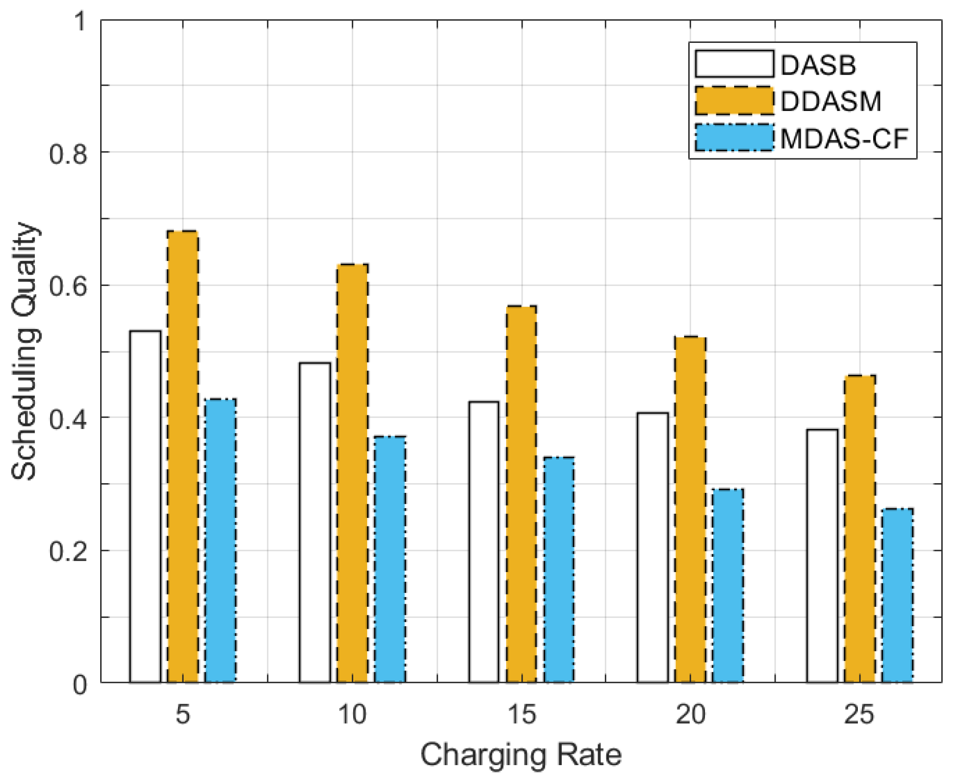
To evaluate the comprehensive performance on multiple objectives, the weighted sum with normalized objective value was adopted as the overall fitness function. The value of the weighted sum is called the scheduling quality, which denotes the quality of optimized scheduling results, and the comparison results on this metric with different charging rates are depicted in Figure 9, where the number of nodes is 40. The lower value of fitness means better quality. When the charging rate reached 25, all scheduling methods obtained were of the best quality, and MDAS-CF was only 57% of DDASM.

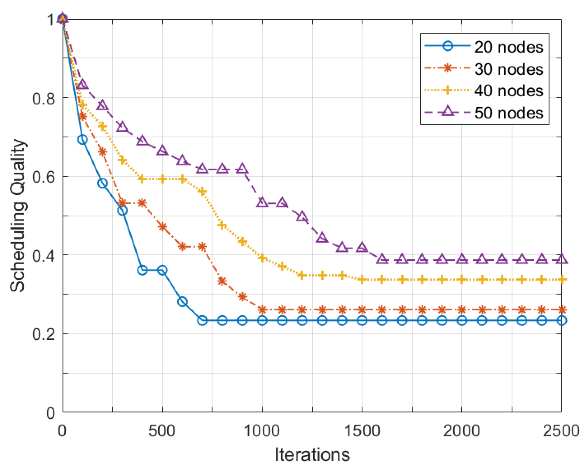
The convergence of scheduling result is an indispensable feature for the scheduling methods based on the chaotic firework algorithm. The stabilization of scheduling quality denotes the convergence state of the proposed method, and the related results can be found in Figure 10. With more nodes in the network, the exploration of the optimal scheduling becomes more complicated, the aggregation delay may increase, and more wireless channels may be occupied. In this case, the convergence time of the scheduling method becomes longer, and the scheduling quality increases as well. When the involved nodes are 50, the method takes about 1600 iterations to reach convergence at about 0.39. Correspondingly, it just takes about 700 iterations to reach convergence at about 0.23 when there are 20 nodes in the network. Even though the exploration of the algorithm may temporarily fall into a local optimal solution during a short period of time, it will rapidly jump out to discover better solutions. For example, when there are 30 nodes in the network, the quality value remains unchanged for the iteration intervals of 400 to 600, but a better solution with a lower quality value is found after 700 iterations.

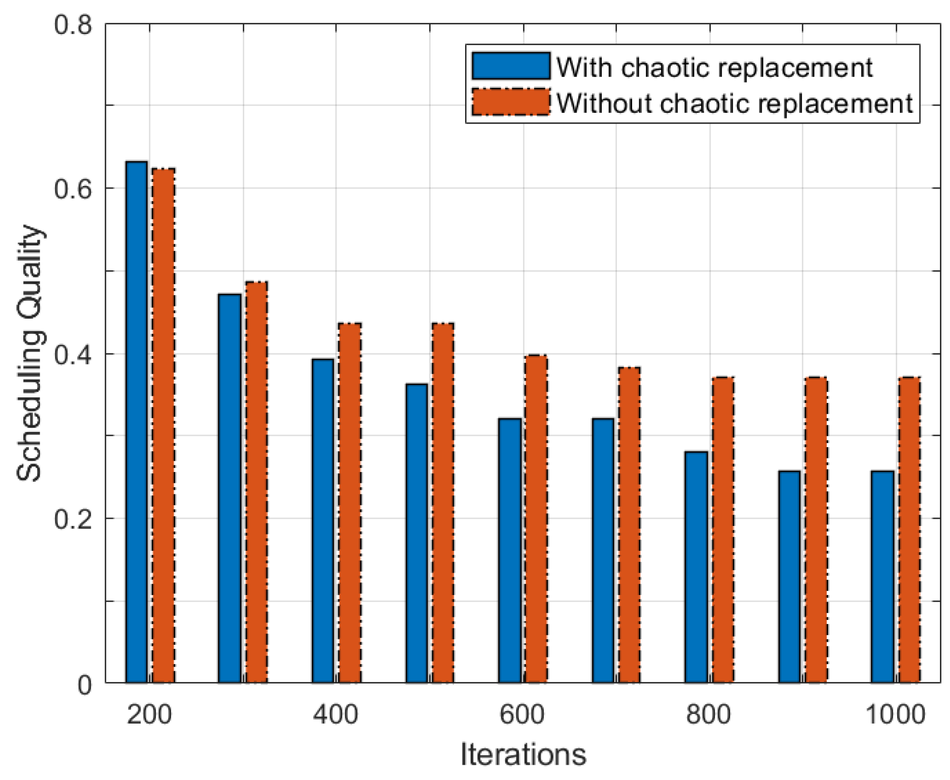
To reflect the role of the chaotic exploration, it is necessary to conduct comparative experiments to verify the improving effect; the results can be found in Figure 11. When the iterations are less than 400, the difference in scheduling quality is not obvious (regarding whether to use chaotic exploration or not). However, the advantage of the chaotic exploration is enhanced along with the increase of the iteration. When the iteration is equal to 1000, the quality without chaotic exploration is about 1.4 times larger than the quality with chaotic exploration.

The chaotic value was generated by the chaotic map function in this research. The chaotic sequence has good ergodicity and randomness, which is beneficial for firework algorithms to get rid of the constraints of local optimal values. An example of the chaotic map function adopted in this paper is depicted in Figure 12, where Figure 12a presents the change of the chaotic value in the range of $[-1,1]$ with parameters $a=1.4,b=2.7$; Figure 12b,c depicts the corresponding results of the Lyapunov exponents and frequency spectrum, respectively.

The parameter $\sigma$ controls the number of firework individuals potentially replaced by the chaotic sequence. In

Table 1. Impact of the parameter $\sigma$ on the scheduling quality.

Periods	$\mathit{\sigma }$ = 0.05	$\mathit{\sigma }$ = 0.1	$\mathit{\sigma }$ = 0.15	$\mathit{\sigma }$ = 0.2
400	0.54	0.48	0.41	0.39
600	0.47	0.39	0.35	0.32
800	0.43	0.39	0.32	0.27

, when $\sigma$ increases to 0.2, the better solution can be discovered. After 800 iterations, the solution quality of the smallest $\sigma$ can drop to about 63% of the solution quality of the largest $\sigma$. However, the larger value of $\sigma$ also indicates much more computation costs, because more chaotic sequences have to be generated and converted to feasible solutions.

MDAS-CF basically obtains better performance on the main optimization objectives, as the simulation results show above. Even though the improved DASB has good performance on the aggregation delay, it takes up excessive channel resources. According to the predefined principle, DDASM distributes the construction task of the scheduling set to each sensor node. Without considering the performance of the overall network, the cooperation of nodes cannot ensure good results on the main performance metrics.

7. Conclusions

To handle the multi-channel data aggregation scheduling problems in battery-free WSNs, the chaotic firework algorithm-based scheduling method was studied in this paper. The target network scenarios and the optimization objectives of scheduling were first analyzed. To solve the scheduling problem, the principle of the chaotic firework algorithm was implemented to the exploration of the optimal scheduling set. The scheduling set was indirectly encoded as the firework individual. With the help of explosion, mutation, and chaotic operations, a sub-optimal scheduling set can be discovered during an acceptable time period. The contrasted experiments were conducted via a network simulation; the simulation results validate the advantage of the proposed method on aggregation delay and occupied channels. In future work, the proposed method will be implemented on real sensor devices and its performance and impact will be evaluated further.

References

1. Shi, T.; Li, J.Z.; Gao, H.; Cai, Z.P. Coverage in battery-free wireless sensor networks. In Proceedings of the IEEE Conference on Computer Communications (IEEE INFOCOM), Honolulu, HI, USA, 16–19 April 2018; pp. 108–116. [Google Scholar]
2. Shi, T.; Li, J.; Gao, H.; Cai, Z. A Novel Framework for the Coverage Problem in Battery-Free Wireless Sensor Networks. IEEE Trans. Mob. Comput. 2022, 21, 783–798. [Google Scholar] [CrossRef]
3. Yao, B.; Gao, H.; Li, J. Multicast Scheduling Algorithms for Battery-Free Wireless Sensor Networks. In Proceedings of the 2019 IEEE 16th International Conference on Mobile Ad Hoc and Sensor Systems (MASS), Monterey, CA, USA, 4–7 November 2019; pp. 398–406. [Google Scholar]
4. Porcarelli, D.; Spenza, D.; Brunelli, D.; Cammarano, A.; Petrioli, C.; Benini, L. Adaptive Rectifier Driven by Power Intake Predictors for Wind Energy Harvesting Sensor Networks. IEEE J. Emerg. Sel. Top. Power Electron. 2015, 3, 471–482. [Google Scholar] [CrossRef]
5. Yi, J.M.; Kang, M.J.; Noh, D.K. Solar Energy Harvesting Wireless Sensor Network Simulator. Int. J. Distrib. Sens. Netw. 2015, 11, 477–485. [Google Scholar] [CrossRef]
6. Lu, X.; Wang, P.; Niyato, D.; Kim, D.I.; Han, Z. Wireless Networks With RF Energy Harvesting: A Contemporary Survey. IEEE Commun. Surv. Tutor. 2015, 17, 757–789. [Google Scholar] [CrossRef]
7. Yahya, N. Agricultural 4.0: Its Implementation Toward Future Sustainability. In Green Urea; Green Energy and Technology; Springer: Berlin/Heidelberg, Germany, 2018. [Google Scholar]
8. Demin, G.; Haifeng, L.; Anna, J.; Guoxin, W. A forest fire prediction system based on rechargeable wireless sensor networks. In Proceedings of the 4th IEEE International Conference on Network Infrastructure and Digital Content, Beijing, China, 19–21 September 2014; pp. 405–408. [Google Scholar]
9. Zalbide, I.; D’Entremont, E.; Jiménez, A.; Solar, H.; Beriain, A.; Berenguer, R. Battery-free wireless sensors for industrial applications based on UHF RFID technology. In Proceedings of the SENSORS, IEEE, Valencia, Spain, 2–5 November 2014; pp. 1499–1502. [Google Scholar]
10. Boubiche, S.; Boubiche, D.E.; Bilami, A.; Toral-Cruz, H. Big Data Challenges and Data Aggregation Strategies in Wireless Sensor Networks. IEEE Access 2018, 6, 20558–20571. [Google Scholar] [CrossRef]
11. Kang, B.; Nguyen, P.K.H.; Zalyubovskiy, V.; Choo, H. A Distributed Delay-Efficient Data Aggregation Scheduling for Duty-Cycled WSNs. IEEE Sensors J. 2017, 17, 3422–3437. [Google Scholar] [CrossRef]
12. Phung, K.H.; Lemmens, B.; Goossens, M.; Nowe, A.; Tran, L.; Steenhaut, K. Schedule-based multi-channel communication in wireless sensor networks: A complete design and performance evaluation. Ad Hoc Netw. 2015, 26, 88–102. [Google Scholar] [CrossRef]
13. Sato, K.; Sakata, S. A Power-Efficient Distributed TDMA Scheduling Algorithm with Distance-Measurement for Wireless Sensor Networks. Wirel. Pers. Commun. 2014, 75, 1511–1528. [Google Scholar] [CrossRef]
14. Ghods, F.; Yousefi, H.; Hemmatyar, A.M.A.; Movaghar, A. MC-MLAS: Multi-channel Minimum Latency Aggregation Scheduling in Wireless Sensor Networks. Comput. Netw. 2013, 57, 3812–3825. [Google Scholar] [CrossRef]
15. Pisanu, T.; Garau, S.; Ortu, P.; Schirru, L.; Macciò, C. Prototype of a Low-Cost Electronic Platform for Real Time Greenhouse Environment Monitoring: An Agriculture 4.0 Perspective. Electronics 2020, 9, 726. [Google Scholar] [CrossRef]
16. Sott, M.K.; Furstenau, L.B.; Kipper, L.M.; Giraldo, F.D.; Lopez-Robles, J.R.; Cobo, M.J.; Zahid, A.; Abbasi, Q.H.; Imran, M.A. Precision Techniques and Agriculture 4.0 Technologies to Promote Sustainability in the Coffee Sector: State of the Art, Challenges and Future Trends. IEEE Access 2020, 8, 149854–149867. [Google Scholar] [CrossRef]
17. Barik, S.; Naz, S. Smart Agriculture Using Wireless Sensor Monitoring Network Powered By Solar Energy. In Proceedings of the International Conference on Computing, Communication, and Intelligent Systems (ICCCIS), Delhi, India, 17–19 February 2021; pp. 983–988. [Google Scholar]
18. Gill, R.; Chawla, P. Energy Harvesting Sensors based Internet of Things System for Precision Agriculture. In Proceedings of the 2nd International Conference on Innovative Practices in Technology and Management (ICIPTM), Gautam Buddha Nagar, India, 18–19 December 2022; pp. 270–273. [Google Scholar]
19. Gulec, O.; Haytaoglu, E.; Tokat, S. A Novel Distributed CDS Algorithm for Extending Lifetime of WSNs With Solar Energy Harvester Nodes for Smart Agriculture Applications. IEEE Access 2020, 8, 58859–58873. [Google Scholar] [CrossRef]
20. Liu, D.; Wu, X.; Cao, Z.; Liu, M.; Li, Y.; Hou, M. CD-MAC: A contention detectable MAC for low duty-cycled wireless sensor networks. In Proceedings of the 12th Annual IEEE International Conference on Sensing, Communication, and Networking (SECON), Seattle, WA, USA, 22–25 June 2015; pp. 37–45. [Google Scholar]
21. Kumar, S.; Kim, H. Energy Efficient Scheduling in Wireless Sensor Networks for Periodic Data Gathering. IEEE Access 2019, 7, 11410–11426. [Google Scholar] [CrossRef]
22. Bagaaa, M.; Younisb, M.; Ksentinic, A.; Badache, N. Reliable Multi-channel Scheduling for timely dissemination of Aggregated data in Wireless Sensor Networks. J. Netw. Comput. Appl. 2014, 46, 293–304. [Google Scholar] [CrossRef]
23. Jiao, X.; Lou, W.; Feng, X.; Wang, X.; Yang, L.; Chen, G. Delay Efficient Data Aggregation Scheduling in Multi-channel Duty-Cycled WSNs. In Proceedings of the IEEE 15th International Conference on Mobile Ad Hoc and Sensor Systems (MASS), Chengdu, China, 9–12 October 2018; pp. 326–334. [Google Scholar]
24. Ren, M.; Li, J.; Guo, L.; Cai, Z. Distributed Data Aggregation Scheduling in Multi-channel and Multi-power Wireless Sensor Networks. IEEE Access 2017, 5, 27887–27896. [Google Scholar] [CrossRef]
25. Lee, J.; Jeong, W. Multi-channel TDMA link scheduling for wireless multi-hop sensor networks. In Proceedings of the International Conference on Information and Communication Technology Convergence (ICTC), Jeju, Korea, 28–30 October 2015; pp. 630–635. [Google Scholar]
26. Zhu, T.; Li, J.; Gao, H.; Li, Y. Data Aggregation Scheduling in Battery-Free Wireless Sensor Networks. IEEE Trans. Mob. Comput. 2022, 21, 1972–1984. [Google Scholar] [CrossRef]
27. Chen, K.; Gao, H.; Cai, Z.; Chen, Q.; Li, J. Distributed Energy-Adaptive Aggregation Scheduling with Coverage Guarantee For Battery-Free Wireless Sensor Networks. In Proceedings of the IEEE Conference on Computer Communications (IEEE INFOCOM), Paris, France, 29 April–2 May 2019; pp. 1018–1026. [Google Scholar]
28. Chen, Q.; Cai, Z.; Cheng, L.; Gao, H. Structure-Free General Data Aggregation Scheduling for Multihop Battery-Free Wireless Networks. IEEE Trans. Mob. Comput. 2021. [Google Scholar] [CrossRef]
29. Cai, Y.; Chen, H.; Qi, Y. Chaotic Fireworks Algorithm for Solving Travelling Salesman Problem. Comput. Sci. 2019, 46, 85–88. [Google Scholar]
30. Luo, W.; Jin, H.; Li, H.; Fang, X.; Zhou, R. Optimal Performance and Application for Firework Algorithm Using a Novel Chaotic Approach. IEEE Access 2020, 8, 120798–120817. [Google Scholar] [CrossRef]
31. Wan, S.; Zhang, Y.; Chen, J. On the Construction of Data Aggregation Tree With Maximizing Lifetime in Large-Scale Wireless Sensor Networks. IEEE Sensors J. 2016, 16, 7433–7440. [Google Scholar] [CrossRef]
32. Chen, X.; Hu, X.; Zhu, J. Minimum data aggregation time problem in wireless sensor networks. In Proceedings of the in Mobile Ad-hoc and Sensor Networks (MSN), First International Conference, Wuhan, China, 13–15 December 2005; pp. 133–142. [Google Scholar]
33. Yu, B.; Li, J.Z. Minimum-Time Aggregation Scheduling in Duty-Cycled Wireless Sensor Networks. J. Comput. Sci. Technol. 2011, 26, 962–970. [Google Scholar] [CrossRef]
34. Zhang, B.; Zheng, Y.J.; Zhang, M.X.; Chen, S.Y. Fireworks Algorithm with Enhanced Fireworks Interaction. IEEE/ACM Trans. Comput. Biol. Bioinform. 2017, 14, 42–55. [Google Scholar] [CrossRef]
35. Zheng, S.; Li, J.; Janecek, A.; Tan, Y. A Cooperative Framework for Fireworks Algorithm. IEEE/ACM Biol. Bioinform. 2017, 14, 27–41. [Google Scholar] [CrossRef] [PubMed]
36. Wang, C.; Liu, X.; Hu, H.; Han, Y.; Yao, M. Energy-Efficient and Load-Balanced Clustering Routing Protocol for Wireless Sensor Networks Using a Chaotic Genetic Algorithm. IEEE Access 2020, 8, 158082–158096. [Google Scholar] [CrossRef]
37. Guillermo, F.; Manuel, V.; Miguel, A. Chaotic genetic algorithm and the effects of entropy in performance optimization. Chaos 2019, 29, 1–7. [Google Scholar]
38. Peng, Y.; Sun, K.; He, S. A discrete memristor model and its application in Hénon map. Chaos Solitons Fractals 2020, 137, 1–6. [Google Scholar] [CrossRef]
39. Liu, J.; Zheng, S.; Tan, Y. Analysis on global convergence and time complexity of fireworks algorithm. In Proceedings of the IEEE Congress on Evolutionary Computation (CEC), Beijing, China, 6–11 July 2014; pp. 3207–3213. [Google Scholar]
Figure 1. Example of symmetric communication.
Symmetry 14 01571 g001
Figure 2. Example of the energy level change on the sensor node.
Symmetry 14 01571 g002
Figure 3. Example of direct and indirect communication conflicts.
Symmetry 14 01571 g003
Figure 4. Example of multi-channel data aggregation scheduling for battery-free WSNs.
Symmetry 14 01571 g004
Figure 5. Example of generating a feasible solution from a priority set.
Symmetry 14 01571 g005
Figure 6. Aggregation delay with different numbers of nodes.
Symmetry 14 01571 g006
Figure 7. Aggregation delay with different charging rates.
Symmetry 14 01571 g007
Figure 8. Occupied channels with different numbers of nodes.
Symmetry 14 01571 g008
Figure 9. Scheduling quality with different charging rates.
Symmetry 14 01571 g009
Figure 10. The convergence of the scheduling method with different numbers of nodes.
Symmetry 14 01571 g010
Figure 11. Comparison between chaotic replacement and non-chaotic replacement.
Symmetry 14 01571 g011
Figure 12. Chaotic waveform, Lyapunov exponents, and frequency spectrum of the chaotic map function.
Symmetry 14 01571 g012