Article

Few-Shot Learning for Fault Diagnosis: Semi-Supervised Prototypical Network with Pseudo-Labels

1
The College of Mechanical Engineering and Automation, Foshan University, Foshan 528011, China
2
The School of Automation, Central South University, Changsha410017, China
*
Author to whom correspondence should be addressed.
Symmetry 2022, 14(7), 1489; https://doi.org/10.3390/sym14071489
Submission received: 30 June 2022 / Revised: 15 July 2022 / Accepted: 19 July 2022 / Published: 21 July 2022

Abstract

:
Achieving deep learning-based bearing fault diagnosis heavily relies on large labeled training samples. However, in real industry applications, labeled data are scarce or even impossible to obtain. In this study, we addressed a challenging few-shot bearing fault diagnosis problem with few or no training labeled samples of novel categories. To tackle this problem, we considered a semi-supervised prototype network based on few-shot bearing fault diagnosis with pseudo-labels. The existing prototypical networks with pseudo-label methods train a pseudo label model to label unlabeled samples using high-dimensional labeled data, which cannot eliminate the instability of the pseudo-label model caused by dimensional labeled features. To mitigate this issue, we used kernel principal component analysis to reduce the dimensions of and remove redundant information from high-dimensional data. Specifically, we used the pseudo-label prediction algorithm with probability distance to label unlabeled samples, aiming to improve the labeling accuracy. We applied two well-known bearing data sets for the validation experiments with symmetry parameters. The findings illustrated that the classification accuracy of the proposed method is higher than that of other existing methods.

1. Introduction

Rotating machinery is an important component of smart manufactory, and its healthy and stability operation are required to guarantee production. However, due to bearings operating long term in harsh environments, then can easily fail, leading to disastrous consequences [1,2]. To ensure the safety and efficiency of smart manufacturing, rolling bearing fault diagnosis needs to be further studied, which has increasingly attracted research attention [3,4].
Benefitting from the rapid development of computer and sensing technologies, industry has entered the era of big data. Due to its big data learning ability, deep learning has replaced shallow models and has been successfully applied in various fields [5,6,7]. With continuous development and improvement, deep-learning models have been widely applied in the field of fault diagnosis. Gong et al. [8] use dan improved convolutional neural network support vector machine (CNN-SVM) method to effectively identify incipient faults in rotation machinery. Jiang et al. [9] explored a deep recurrent neural network (DRNN) to automatically extract the features from input spectrum sequences. Cui et al. [10] proposed a feature distance stack autoencoder (FD-SAE) for rolling bearing fault diagnosis to improve the feature extraction ability and the convergence speed of the network. Zhang et al. [11] combined an ensemble deep belief network and variation mode decomposition to improve the accuracy and stability of the diagnosis of the health status of rotating machinery. These existing methods, which are based on deep learning, can produce accurate results; however, a large amount of labeled data are required to obtain an effective deep model. However, obtaining enough labeled samples in actual industrial applications is difficult and time-consuming. Therefore, more effort is needed to apply few-shot learning to solving the problems encountered in the practical application of deep-learning methods.
Few-shot learning, a technique of learning from a few labeled samples for automatically classifying massive amounts unlabeled samples, has recently attracted attention. Zhang et al. [12] proposed a few-shot learning approach for fault diagnosis under limited data conditions based on CNNs and Siamese neural networks. Jiang et al. [13] embedded a two-branch network into the prototype network, building a two-branch prototype network fault diagnosis method to mitigate the few-shot samples classification issue. Xu et al. [14] combined K-nearest neighbor with cosine distance to build a distribution discrepancy metric and developed a deep convolutional nearest neighbor matching network for few-shot learning. Wang et al. [15] developed a feature space metric-based meta-learning model to overcome the challenge produced by few-shot learning problem under limited labeled samples by adopting both individual sample information and similarity sample group information. Xu et al. [16], based on approximation space and belief functions, design edan few-shot learning method for fault diagnosis. They used the basic probability assignment calculation to build belief functions for diagnosis within sufficient information. Although these existing few-shot learning fault diagnosis methods achieve encouraging fault diagnosis performance in the conditions with few labeled samples, these existing few-shot methods ignore the massive unlabeled data that exist in practical industrial applications, which may be used aspseudo-labels in combination with the few labeled samples to effectively train deep-learning models.
Semi-supervised few-shot learning, as a promising method for labeled samples, is increasingly receiving research attention. Tao et al. [17] designed a bearing defect diagnosis model using pseudo-labels, which obtained representative features for classification from unlabeled samples. Zhang et al. [18] used a Monte Carlo uncertainty threshold selection strategy to increase the confidence of the pseudo-labels, then used a momentum prototype network to obtain the feature space mapping using few labeled samples. Yong et al. [19] used an encoder to extract features for training prototypes, then semi-supervised meta-learning, which they optimized by a combinatorial learning optimizer to refine original prototypes from unlabeled samples. Kai et al. [20] explored a pseudo-loss confidence metric for task-unified confidence estimation through mapping the different pseudo-labels to the same metric space using of the pseudo-loss. Di et al. [21] combined learner of latent representations with cluster structures, and proposed a pseudo-label-guided collective matrix factorization method for multi-view clustering. More recently, these semi-supervised few-shot learning methods have been widely studied, and encouraging results have been obtained. However, most of these existing methods focus on the confidence estimation inference of pseudo-label learning, which suffers when samples in a single task are insufficient, and ignore the redundant information embedded into feature space, which can cause errors in pseudo-label learning models, considerably decreasing the generalization capability of a model.
In an effort to achieve the semi-supervised few-shot learning, and motivated by the aforementioned analysis, and considering the influence of the redundant information in high-dimensional feature space, we designed a kernel principal component analysis method based on a semi-supervised prototypical network for fault diagnosis with pseudo-labels. We used kernel principal component analysis to reduce the dimensions of the feature space, which mitigates the effects of redundant information and results in a lightweight training model. We used the pretrained model, whose parameters we obtained by training model with these features through dimension reduction, to predict the labels of unlabeled data, and we selected the reliable labels as the pseudo-labels. We sent the pseudo-labeled data to the pretrained prototype networks to further fine tune the parameters to produce prototype networks with strong generalization ability. Finally, we conducted comparison experiments based on two well-known bearing datasets (Case Western Reserve University, CWRU) to prove the effectiveness of our method.
The main highlights of the study are as follows:
(1)
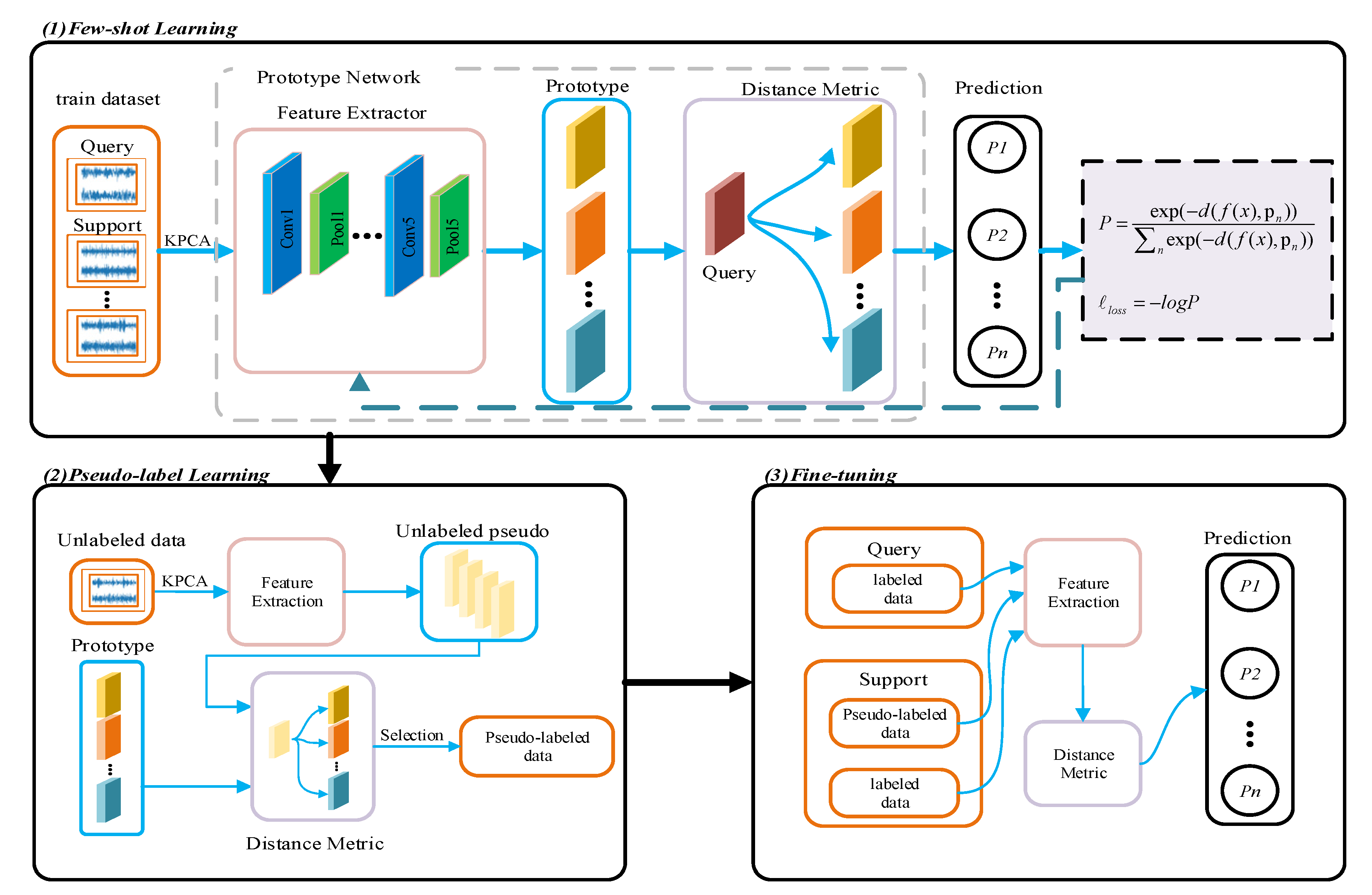
We used kernel principal component analysis to reduce the dimension of the feature space, which avoid redundant information embedded in the feature space reducing the generalization ability of the model;
(2)
We used apseudo-label-prediction algorithm to generate labeled samples, aiming to increase the labeled samples, which fully uses the unlabeled samples for training the prototype networks to avoid overfitting;
(3)
We adopted predicted pseudo-label data to fine tune the prototype network parameters, which can reduce the time required for adjusting the model parameters and improves diagnostic accuracy.

2. Theoretical Background

2.1. Few-Shot Learning

Few-shot learning [22], which aims to learn about a new category from a small amount of labeled data, has aroused increased interest in the pattern recognition community. This technique has been extensively applied in artificial intelligence.
In the few-shot learning problem, all datasets are divided into three parts: the support set S = { ( x i s , y i s ) } i = 1 n s ( n s = C × N , x i R D ) , query set Q = { ( x i q , y i q ) } i = 1 n q ( n q = 1 × N , x i R D ) , and test set T = { ( x i t , y i t ) } i = 1 n t , where the data of support and query sets are from the same class, and the samples in the two sets are different. The sample categories of the test set differ from those of the support set. x i R D denote the feature vector extracted from a raw vibration signal; y i { 1 , 2 , , C } denotes the label of the dataset samples. In the traditional method, the dataset is only divided into a training and a test set. Compared with the traditional method, the support set S and query set Q are used to train the network, and the test set T   is   used   to evaluate the performance of the network, which improves the stability and generalization of the model. If the support set contains N classes and K samples, it can be described as an N-way K-shot problem. The process of few-shot learning is illustrated in Figure 1.

2.2. Prototypical Network

Prototypical networks [23,24] generalize new classes not included in the training set given only a small number of examples of each new class. Metric-based few-shot learning has been widely used in few-shot learning, producing impressive results. An embedding function is obtained by a neural network through prototypical network learning; then, samples are extracted into feature vectors. The mean vectors in each class are the prototype. During classification, query samples are first transformed into feature vectors; the distance from the vector to the prototypes represents the similarity to the class. Figure 2 describes the working of the prototype networks.
In few-shot learning, a support set of N labeled samples S = { ( x 1 , y 1 ) , ( x n , y n ) } is given, where each x i R D is the dimensional feature vector D, and y i { 1 , , K } is the label of x i . S k denotes k classes in the support set. Through an embedding function f ϕ R D R M , prototype p k is computed as follows:
p k = 1 | S k | ( x i , y i ) S k f ϕ ( x i )
During the classification, distance is calculated by the distance function d ( · ) ; the probability that query point X belongs to class K can be expressed as:
P ϕ ( y = k | x ) = log ( exp ( d ( f ϕ ( x ) , p k ) ) k exp ( d ( f ϕ ( x ) , p k ) ) )

3. Proposed Method

3.1. KPAC

KPCA is a non-linear derivative of PCA that can be solved as an eigenvalue problem of its kernel matrix [25]. Samples are non-linearly mapped into higher-dimensional feature space F , and PCA is performed there.
Let sample x 1 , , x   N R D be mapped into Φ ( x 1 ) , , Φ ( x n ) F . The covariance matrix C in the feature space F is given by:
C = 1 N k = 1 N Φ ( x k ) Φ ( x k ) T
where k = 1 N Φ ( x k ) = 0 . Non-zero eigenvalues λ of te covariance matrix C can be calculated as:
λ v = C v
where v denotes the corresponding eigenvector of F , which can also be written as:
v = k = 1 N α k Φ ( x k )
The problem is simplified to find the coefficient l k , which can be formulated as the following eigenvalue problem by substituting Equations (3) and (5) into (4), which is written as:
K α = N λ α
where K is a kernel matrix with size N × N , which can calculated as follows:
K i j = ( Φ ( x i ) · Φ ( x j ) ) = k ( x i , x j )
k ( · ) denotes the kernel function, which is used to calculate the inner product of Φ ( x i ) and Φ ( x j ) . In this study, we used the RBF kernel function:
k ( x i , x j ) = exp ( x i x j 2 2 σ 2 )
where σ is set to 1 / N . Let λ l be the l th largest eigenvalue of K , and α l = [ α 1 l , ,   α 1 N ] be the corresponding eigenvector. An input sample x   can be mapped onto the l   th dimension of KPCA space with coordinate value:
v l , Φ ( x ) = i = 1 N α i l k ( x i , x )
The advantage of kernel principal component analysis is that only the kernel function needs to be calculated in the original space; the nonlinear mapping function Φ ( x ) does not need to be known.

3.2. Metric and Query

In this study, we used the Euclidean distance to calculate the similarity of samples through the feature vectors extracted from these samples. The distance can be represented as:
d f ( p n , x i q ) = f ( p n ) f ( x i q )
where p n denotes the prototype of class n, x i q denotes the ith sample in query set, and f ( · ) is the feature vector extracted from the raw vibration signal. The smaller the distance d f , the more similar the query data to this class. The probability of the sample from query set   x i q   belonging to class k can be described as:
P ( y = k | x i q ) = exp ( d ( f ( x ) , p n ) ) n exp ( d ( f ( x ) , p n ) )
In the process of pseudo-label learning, to retain samples with good classification performance, we used the experimental data to verify that, after SoftMax function screening, the samples whose probability value was greater than 0.7 had high classification accuracy. The detailed experiment of probability P is illustrated in Figure 3.
Then, the loss function of the samples selected for the query set was designed as:
l o s s = log P ( y = k | x i q )

3.3. Description of Proposed Method

In this study, we designed a kernel principal analysis based semi-supervised prototypical network (PSSPN). The whole algorithm is described in Algorithm 1.
Algorithm 1: PSSPNlearning strategy
Input: Labeled dataset D L , unlabeled dataset D U , number of fault classes N , support set S e with K samples query set Q e with Q samples, feature extractor f φ episode, and epoch.
Output: learnable parameter φ
  • Preprocess the raw data with KPCA
  • For each epoch, do:
  • Randomly sample N classes in dataset D L ; each class has K samples THAT consist of support set S e . Similarly, randomly sample Q samples to create query set Q e .
  • Obtain samples x i S and x i Q from support set S e and query set Q e , respectively, and generate support feature set f φ ( x i S ) and query feature set f φ ( x i Q ) .
  • Generate prototype P k by Equation (1).
  • Calculate the classification probability P ( y = k | x i q ) by Equation (2).
  • Calculate the loss, and update parameter φ .
  • Use the model pretrained in steps 2–8 to predict the label of D U ; after selection, we obtain the pseudo-labeled dataset D p s e u d o .
  • Fine-tune parameter φ with datasets D p s e u d o and D L .
  • End
Step (1)—Few-shot learning: the dimensions of the labeled data feature space are reduced by KPCA. Then, feed this reduced-dimension feature space into the prototypical network. Calculate the distance between samples in the query set and prototype. Then, convert the similar distances into probability values using a SoftMax classifier. Calculate the loss and update the parameters of the network. After iterating, the pretrained model is obtained.
Step (2)—Unlabeled samples data are preprocessed by KPCA: through the pretrained model, obtain the predicted label of the unlabeled data. After selection, retain part of the label, and then obtain the pseudo-labeled data.
Step (3)—Input the predicted pseudo-label samples to the labeled sample set to train and fine-tune the relevant parameters of the prototypical network.
A detailed description of the workflow of the proposed method is provided in Figure 4.

4. Results and Discussion

We used three methods, CNN, ProtoNet [24], and improved prototype network(IPN) [26], for a comparison experiment to verify the validity of the proposed method. The feature extractors of CNN and ProtoNet have the same network structure. IPN uses L2 regularization and a dropout layer, which help to address model overfitting problem. The architecture of PSSPN is described in detail in Table 1. We use leaky ReLU as the activation function, and α is 0.3. The network is optimized by the Adam optimizer, whose learning rate is 0.001. We repeated the experiment 20 times to obtain the final accuracy. We used Tensorflow 2.0 to conduct the experiment.

4.1. Case Study on CWRU

4.1.1. Description of CWRU

In this study, we used the Case Western Reserve University (CWRU) bearing datasets [27], which were collected under four different working conditions and loads (0, 1, 2, and 3 hp); the motor worked at speeds of 1979, 1772, 1750, and 1730 rpm, respectively. Each working condition had four bearing fault conditions: normal, ball fault, inner race fault, and outer race fault. Each fault type contained three fault sizes: 0.007, 0.014, and 0.021 inches. We provide details about the dataset in Table 2, which shows that there were 10 types in total. For the detailed experimental platform, please refer to the related references.
We generated all the training and testing samples using a sliding window. We set the sliding window to 1024, and step length of the framing to 80. The detailed information about the dataset used in the experiment is provided in Table 3.

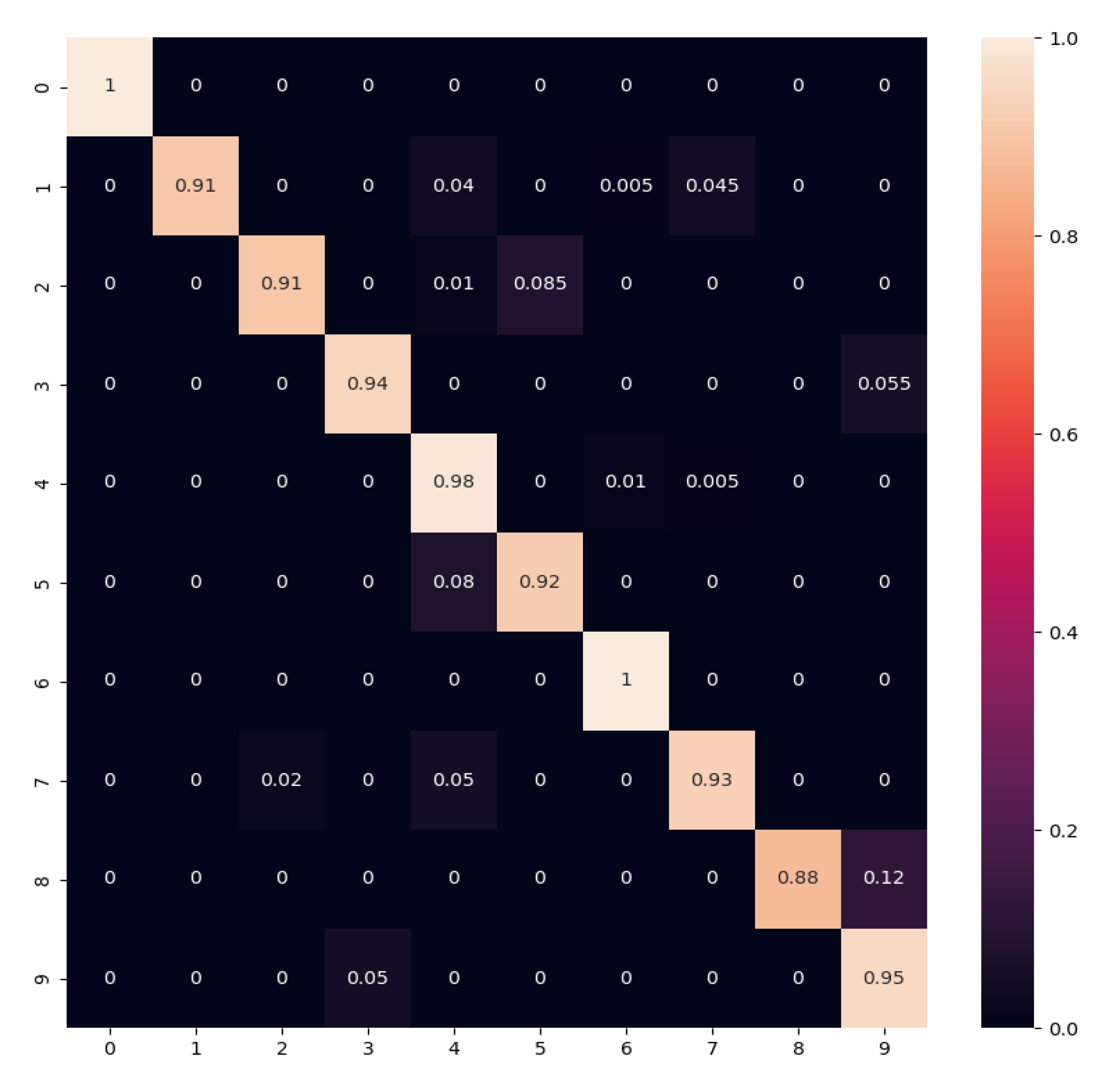
4.1.2. Results Analysis

In this case, study, 1-shot and 5-shot experiment is conducted on the dataset descripted as Table 3, all parameters of compared methods are mentioned above, and the experiment result is listed in Table 4
Table 4 shows that the classification accuracies of the few-shot learning methods are much higher than that of conventional CNN. For 1-, 5-, and 10-shot learning, the PSSPN achieved 89.72%, 94.65%, and 97.05% accuracies, respectively, which are higher than those of the other considered methods. The classification accuracy of ProtoNet with KPCA is higher than that of ProtoNet. This finding showed that KPCA helps remove redundant information, which cause errors in the model during training.
Figure 5 shows the confusion matrix for the five-shot classification accuracy result of PSSPN. We found that the We generated accuracy of PSSPN was high for various bearing fault types. However, for label 8, the classification accuracy was relatively low, and several samples were categorized into label 9. The most probable reason for this is that the difference between these two samples is small, which lead to misclassification. With the increase in the number of training samples, the classification accuracy of the various methods also increased, especially that of ProtoNet and IPN. The classification accuracy of PSSPN was higher when the number of labeled training samples was small.
Figure 6 illustrates the feature visualization produced for t-SNE. In CNN, the difference in some classes was clear, but several features were indivisible. In ProtoNet and IPN, different samples were successfully distinguished, but the result was messy. The results produced by PSSPN were more clearly divided than that of the other considered methods, though the boundaries of some samples were ambiguous. Possible reasons for this include the amount of data being relatively small, and the model could not be further improved; or the difference between the samples being small, and our model could not distinguish this gap.

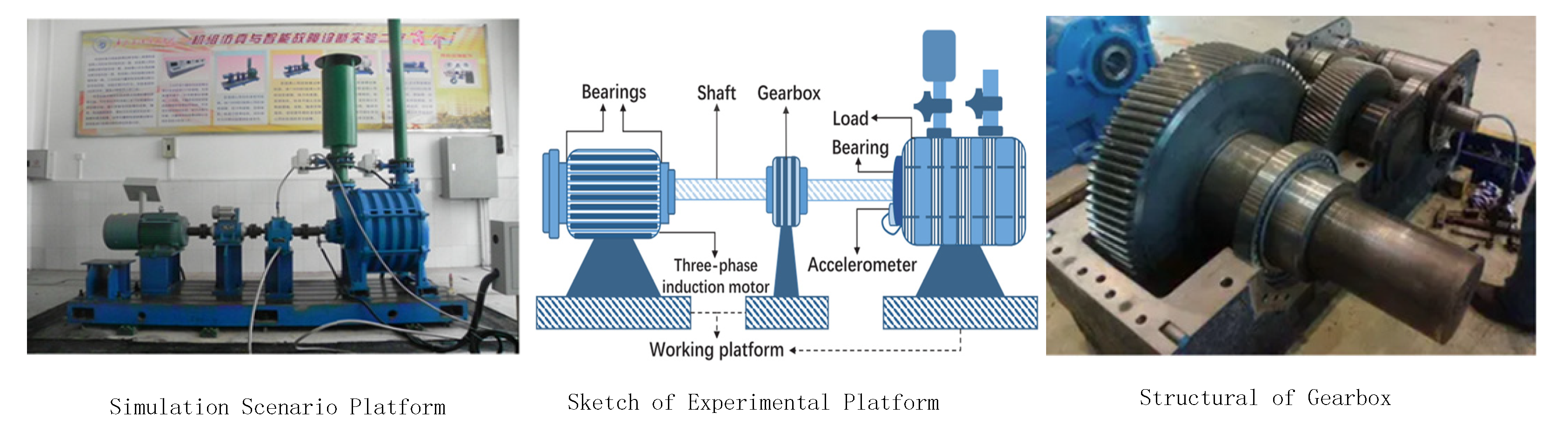
4.2. Case Study on Petrochemical Dataset

4.2.1. Petrochemical Dataset Introduction

The petrochemical dataset(Guangdong Provincial Key Laboratory of Petrochemical Equipment Fault Diagnosis, Guangdong University of Petrochemical Technology, Maoming, China) [29,30] contains more noise and is related to industrial environments. We established a simulation platform to simulate the actual working environment of a petrochemical refinery and the power load of rotating machinery. The detailed information of the platform used for data collection from the machinery is provided in Figure 7. For more detailed information, please refer to the provided references.
The fault types in the petrochemical dataset are as follows: (1) F0: gearwheels are missing teeth; (2) F1: gearwheels are missing teeth and the outer ring of the left-side bearing is worn; (3) F2: gearwheels are missing teeth and inner ring of the left-side bearing is worn; (4) F3: gearwheels are missing teeth and the balls on the left-side bearing are missing; (5) F4: pinion and gearwheels are missing teeth; and (6) F5: object is in a normal state. The detailed information about the dataset we used in our experiments are provided in Table 5.

4.2.2. Six-Way Fault Classification

The petrochemical dataset has six fault classes, and each sample has 1024 sampling points. In this case, study experiment, we chose 500 samples for training, and 1000 unlabeled samples and 200 labeled samples for evaluation. Detailed dataset information is listed in Table 5. The parameters of the model were the same as used for CWRU dataset. We determined the classification accuracy of all considered methods, as provided in Table 6.
As shown in Table 6, compared with the other few-shot learning strategies, the lowest classification accuracy was obtained by CNN. However, both ProtoNet and IPN achieved accurate classification. In 10- and 30-shot, IPN reached 100% classification accuracy. Adding KPCA, the accuracy of slightly ProtoNet improved. For of one- and five-shot learning, PSSPN performed the best, showing that the model can deal with the situations when data are scarce.
The confusion matrix of five-shot classification accuracy is shown in Figure 8. Many samples were correctly classified, and the average classification accuracy was 96.2%.
Figure 9 shows feature visualization via t-SNE, showing that CNN could not clearly distinguish different fault classes. ProtoNet and IPN performed better thanCNN: the distance between features of different classes was as large as possible and the features in the same classes were close to each other. However, some features from different classes were still close to each other. Our proposed method is relatively more accurate than the others in t-SNE. In our method, different classes have well-defined boundaries.

5. Conclusions

We presented a kernel principal component analysis method with a semi-supervised prototype network (PSSPN) for few-shot bearing fault diagnosis. This method can be used when few labeled samples are available and makes full use of the unlabeled data to train the model. KPCA is used for avoiding the dimensionality problem to improve the accuracy of the classification results. We used pseudo-labeled data to fine-tune the pretrained model to avoid the problem of model overfitting. We used two datasets to evaluate the performance of the proposed method, and the results showed that compared with two other methods, the classification accuracy of our proposed method is higher when few labeled samples are available. In the future, we will improve the model to deal with data that are difficult to distinguish and increase the accuracy of the classification result.

Author Contributions

Methodology and Writing—Original draft preparation, J.H.; software and validation, Z.Z.; funding acquisition and supervision, X.F.; formal analysis, Y.C.; investigation and writing—review and editing, D.C.; resources and data curation, S.L. All authors have read and agreed to the published version of the manuscript.

Funding

This research was funded by the National Natural Science Foundation of China with grants 61703104 and 62173349; Key Laboratory of High Performance Complex Manufacturing with grant ZZYJKT2020-14; and Hunan Provincial Key Laboratory with grant 2017TP1002.

Institutional Review Board Statement

Not applicable.

Informed Consent Statement

Not applicable.

Data Availability Statement

MDPI Research Data Policies.

Conflicts of Interest

The authors declare no conflict of interest.

References

  1. Liu, R.; Yang, B.; Zio, E.; Chen, X. Artificial intelligence for fault diagnosis of rotating machinery: A review. Mech. Syst. Signal Process. 2018, 108, 33–47. [Google Scholar] [CrossRef]
  2. Zhou, D.H.; Zhao, Y.H.; Wang, Z.D.; He, X.; Gao, M. Review on Diagnosis Techniques for Intermittent Faults in Dynamic Systems. IEEE Trans. Ind. Electron. 2020, 67, 2337–2347. [Google Scholar] [CrossRef]
  3. Rai, A.; Upadhyay, S.H. A review on signal processing techniques utilized in the fault diagnosis of rolling element bearings. Tribol. Int. 2016, 96, 289–306. [Google Scholar] [CrossRef]
  4. He, J.; Ouyang, M.; Chen, Z.; Chen, D.; Liu, S. A Deep Transfer Learning Fault Diagnosis Method Based on WGAN and Minimum Singular Value for Non-Homologous Bearing. IEEE Trans. Instrum. Meas. 2022, 71, 1–9. [Google Scholar] [CrossRef]
  5. Qin, S.; Jiang, T. Improved Wasserstein conditional generative adversarial network speech enhancement. EURASIP J. Wirel. Commun. Netw. 2018, 2018, 181. [Google Scholar] [CrossRef]
  6. Zhu, L.; Chen, Y.; Ghamisi, P.; Benediktsson, J.A. Generative Adversarial Networks for Hyperspectral Image Classification. IEEE Trans. Geosci. Remote Sens. 2018, 56, 5046–5063. [Google Scholar] [CrossRef]
  7. Yin, H.; Li, Z.; Zuo, J.; Liu, H.; Yang, K.; Li, F. Wasserstein Generative Adversarial Network and Convolutional Neural Network (WG-CNN) for Bearing Fault Diagnosis. Math. Probl. Eng. 2020, 2020, 2604191. [Google Scholar] [CrossRef]
  8. Gong, W.; Chen, H.; Zhang, Z.; Zhang, M.; Wang, R.; Guan, C.; Wang, Q. A novel deep learning method for intelligent fault diagnosis of rotating machinery based on improved CNN-SVM and multichannel data fusion. Sensors 2019, 19, 1693. [Google Scholar] [CrossRef] [Green Version]
  9. Jiang, H.; Li, X.; Shao, H.; Zhao, K. Intelligent fault diagnosis of rolling bearings using an improved deep recurrent neural network. Meas. Sci. Technol. 2018, 29, 065107. [Google Scholar] [CrossRef]
  10. Cui, M.; Wang, Y.; Lin, X.; Zhong, M. Fault diagnosis of rolling bearings based on an improved stack autoencoder and support vector machine. IEEE Sens. J. 2020, 21, 4927–4937. [Google Scholar] [CrossRef]
  11. Zhang, C.; Zhang, Y.; Hu, C.; Liu, Z.; Cheng, L.; Zhou, Y. A novel intelligent fault diagnosis method based on variational mode decomposition and ensemble deep belief network. IEEE Access 2020, 8, 36293–36312. [Google Scholar] [CrossRef]
  12. Zhang, A.; Li, S.; Cui, Y.; Yang, W.; Dong, R.; Hu, J. Limited data rolling bearing fault diagnosis with few-shot learning. IEEE Access 2019, 7, 110895–110904. [Google Scholar] [CrossRef]
  13. Jiang, C.; Chen, H.; Xu, Q.; Wang, X. Few-shot fault diagnosis of rotating machinery with two-branch prototypical networks. J. Intell. Manuf. 2022. [Google Scholar] [CrossRef]
  14. Xu, J.; Xu, P.; Wei, Z.; Ding, X.; Shi, L. DC-NNMN: Across Components Fault Diagnosis Based on Deep Few-Shot Learning. Shock. Vib. 2020, 2020, 3152174. [Google Scholar] [CrossRef]
  15. Wang, D.; Zhang, M.; Xu, Y.; Lu, W.; Yang, J.; Zhang, T. Metric-based meta-learning model for few-shot fault diagnosis under multiple limited data conditions. Mech. Syst. Signal Process. 2021, 155, 107510. [Google Scholar] [CrossRef]
  16. Xu, Y.; Li, Y.; Wang, Y.; Zhong, D.; Zhang, G. Improved few-shot learning method for transformer fault diagnosis based on approximation space and belief functions. Expert Syst. Appl. 2021, 167, 114105. [Google Scholar] [CrossRef]
  17. Tao, X.; Ren, C.; Li, Q.; Guo, W.; Liu, R.; He, Q.; Zou, J. Bearing defect diagnosis based on semi-supervised kernel Local Fisher Discriminant Analysis using pseudo labels. ISA Trans. 2021, 110, 394–412. [Google Scholar] [CrossRef]
  18. Zhang, X.; Su, Z.; Hu, X.; Han, Y.; Wang, S. Semi-supervised momentum prototype network for gearbox fault diagnosis under limited labeled samples. IEEE Trans. Ind. Inform. 2022, 18, 6203–6213. [Google Scholar] [CrossRef]
  19. Feng, Y.; Chen, J.; Zhang, T.; He, S.; Xu, E.; Zhou, Z. Semi-supervised meta-learning networks with squeeze-and-excitation attention for few-shot fault diagnosis. ISA Trans. 2021, 120, 383–401. [Google Scholar] [CrossRef]
  20. Huang, K.; Geng, J.; Jiang, W.; Deng, X.; Xu, Z. Pseudo-loss Confidence Metric for Semi-supervised Few-shot Learning. In Proceedings of the 18th IEEE/CVF International Conference on Computer Vision (ICCV), Montreal, BC, Canada, 11–17 October 2021; pp. 8651–8660. [Google Scholar]
  21. Wang, D.; Han, S.; Wang, Q.; He, L.; Tian, Y.; Gao, X. Pseudo-Label Guided Collective Matrix Factorization for Multiview Clustering. IEEE Trans. Cybern. 2021. [Google Scholar] [CrossRef]
  22. Sung, F.; Yang, Y.; Zhang, L.; Xiang, T.; Torr, P.H.S.; Hospedales, T.M. Learning to Compare: Relation Network for Few-Shot Learning. In Proceedings of the 31st IEEE/CVF Conference on Computer Vision and Pattern Recognition (CVPR), Salt Lake City, UT, USA, 18–23 June 2018; pp. 1199–1208. [Google Scholar]
  23. Pan, Y.; Yao, T.; Li, Y.; Wang, Y.; Ngo, C.-W.; Mei, T.; Soc, I.C. Transferrable Prototypical Networks for Unsupervised Domain Adaptation. In Proceedings of the 32nd IEEE/CVF Conference on Computer Vision and Pattern Recognition (CVPR), Long Beach, CA, USA, 16–20 June 2019; pp. 2234–2242. [Google Scholar]
  24. Snell, J.; Swersky, K.; Zemel, R. Prototypical Networks for Few-shot Learning. In Proceedings of the 31st Annual Conference on Neural Information Processing Systems (NIPS), Long Beach, CA, USA, 4–9 December 2017. [Google Scholar]
  25. Varon, C.; Alzate, C.; Suykens, J.A.K. Noise Level Estimation for Model Selection in Kernel PCA Denoising. IEEE Trans. Neural Netw. Learn. Syst. 2015, 26, 2650–2663. [Google Scholar] [CrossRef] [PubMed]
  26. Ji, Z.; Chai, X.; Yu, Y.; Pang, Y.; Zhang, Z. Improved prototypical networks for few-Shot learninge. Pattern Recognit. Lett. 2020, 140, 81–87. [Google Scholar] [CrossRef]
  27. Smith, W.A.; Randall, R.B. Rolling element bearing diagnostics using the Case Western Reserve University data: A benchmark study. Mech. Syst. Signal Process. 2015, 64–65, 100–131. [Google Scholar] [CrossRef]
  28. Tian, X.; Chen, L.; Zhang, X.; Chen, E. Improved prototypical network model for forest species classification in complex stand. Remote Sens. 2020, 12, 3839. [Google Scholar] [CrossRef]
  29. Zhang, J.; Zhang, Q.; He, X.; Sun, G.; Zhou, D. Compound-Fault Diagnosis of Rotating Machinery: A Fused Imbalance Learning Method. IEEE Trans. Control Syst. Technol. 2021, 29, 1462–1474. [Google Scholar] [CrossRef]
  30. Hu, Q.; Qin, A.; Zhang, Q.; He, J.; Sun, G. Fault Diagnosis Based on Weighted Extreme Learning Machine with Wavelet Packet Decomposition and KPCA. IEEE Sens. J. 2018, 18, 8472–8483. [Google Scholar] [CrossRef]
Figure 1. N-way K-shot learning problem description.
Symmetry 14 01489 g001
Figure 2. Schematic diagram of prototype network.
Symmetry 14 01489 g002
Figure 3. Probability P vs. the classification accuracy.
Symmetry 14 01489 g003
Figure 4. Fault diagnosis framework of the proposed method.
Symmetry 14 01489 g004
Figure 5. Confusion matrix for 5-shot classification result produced by PSSPN in this case study.
Symmetry 14 01489 g005
Figure 6. t-SNE visualization produced by different methods in this case study.
Symmetry 14 01489 g006
Figure 7. Platform of petrochemical motor.
Symmetry 14 01489 g007
Figure 8. Confusion matrix results for 5-shot classification.
Symmetry 14 01489 g008
Figure 9. T-SNE visualization of different methods.
Symmetry 14 01489 g009
Table 1. Feature extractor network description.
No.Layer TypeKernel
Size/Stride
Kernel
Number
Output Size
(Width × Depth)
Padding
1Conv13 × 1/1 × 116256 × 16same
2Pool12 × 1/1 × 116128 × 16valid
3Conv23 × 1/1 × 132128 × 32same
4Pool22 × 1/1 × 13264 × 64valid
5Conv33 × 1/1 × 16432 × 64same
6Pool32 × 1/1 × 16416 × 64valid
7Conv43 × 1/1 × 16416 × 64same
8Pool42 × 1/1 × 1646 × 64valid
9Conv53 × 1/1 × 1646 × 64same
10Pool52 × 1/1 × 1643 × 64valid
Table 2. Bearing health states in CWRU dataset.
StateDescriptionFault Size (Inches)
NNormal condition
RFFault on roller0.007, 0.014, 0.021
IFFault on inner race0.007, 0.014, 0.021
OFFault on te out race0.007, 0.014, 0.021
Table 3. Information about dataset used in our experiments.
Fault LocationNoneBallInner RaceOuter RaceLoad
Fault Diameter (Inches)
Fault Labels
00.0070.0140.0210.0070.0140.0210.0070.0140.024
12345678910
DatasetPretrain5005005005005005005005005005001
Unlabeled1000100010001000100010001000100010001000
Test200200200200200200200200200200
Table 4. The classification accuracy of methods based on CWRU.
MethodsCWRU
1-Shot5-Shot10-Shot15-Shot30-Shot
CNN18.88 ± 0.2380.58 ± 0.3880.36 ± 0.5480.09 ± 0.0780.32 ± 0.17
ProtoNet [24]83.06 ± 0.7789.80 ± 0.3292.27 ± 0.2399.81 ± 0.0299.85 ± 0.01
IPN [28]85.97 ± 0.4389.97 ± 0.2393.36 ± 0.3199.59 ± 0.0399.28 ± 0.05
ProtoNet+KPCA85.12 ± 0.5892.03 ± 0.2395.88 ± 0.1096.30 ± 0.1396.26 ± 0.09
PSSPN (ours)89.72 ± 0.3894.65 ± 0.1697.05 ± 0.0795.92 ± 0.1096.59 ± 0.07
Table 5. Description of petrochemical dataset.
Fault LocationF0F1F2F3F4
Fault Label012345
DatasetPretrain500500500500500500
Unlabeled100010001000100010001000
Test200200200200200200
Table 6. Classification accuracy of all considered methods.
MethodPetrochemical Dataset
1-Shot5-Shot10-Shot15-Shot30-Shot
CNN41.46 ± 0.1676.63 ± 0.4192.84 ± 0.0182.79 ± 0.1491.78 ± 0.24
ProtoNet [24]86.79 ± 0.5394.07 ± 0.1897.04 ± 0.0697.56 ± 0.1497.71 ± 0.29
IPN [28]88.86 ± 2.2089.12 ± 1.91100100100
ProtoNet+KPCA88.70 ± 0.3895.35 ± 0.0798.38 ± 0.0798.30 ± 0.0499.17 ± 0.20
PSSPN89.61 ± 0.3096.23 ± 0.0697.77 ± 0.0898.57 ± 0.0497.30 ± 0.03
Publisher’s Note: MDPI stays neutral with regard to jurisdictional claims in published maps and institutional affiliations.

