Exact Traveling Wave Solutions in a Generalized Harry Dym Type Equation

Abstract

The traveling wave solutions of a generalized HD type equation are investigated in this study. The traveling wave system is a singular system of the first class with given parameter conditions. From the standpoint of dynamical systems, the bifurcations of traveling wave solutions in parameter space are examined. It is demonstrated that solitary wave solutions, periodic peakons, pseudo-peakons, and compacton solutions exist. All conceivable exact explicit parametric representations of various solutions are presented.

1. Introduction

In 1993, Camassa and Holm found that CH-equation [1] $m_t+u{m}_x+2u_{x}m=0,$$m=u-u_{xx}$ has a peakon solution $u(x,t)=c{e}^{-|x-ct|},c\in R.$ In the past thirty years, for the studies of peakon solutions in nonlinear wave equations, a lot of papers have been published (see [2,3,4] and references therein). Peakon is a special traveling wave solution. In [5], Li and Qiao defined a concept of pseudo-peakon. Li and Chen in [4,6] generally considered a class of singular traveling systems. They demonstrated that periodic peakon is a smooth classical solution of a solitary traveling system with two time-scales. Under two classes of limit senses, a peakon is a limit solution of a family of periodic peakons or a limit solution of a family of pseudo-peakons (see [7]). The compacton family is a singular system solution family in which all solutions have finite sets of support, i.e., the defined region of each solution with respect to the variable is finite and the wave function’s value region is bounded. In [4,6,8], a categorization for different wave profiles of solutions was offered, corresponding to different types of phase orbits.

In 2015, as a nonlinear generalization of the equation with pseudo-peakon solutions, ref. [9] proposed a hierarchy of a generalized Harry Dym type ($gHD$ type) equations (see [10,11]). A typical member in the hierarchy reads

$$u_t=2{\left(u^{-\frac{1}{2}}\right)}_{xxx}+2\tau {\left(u^{\frac{3}{2}}\right)}_x,$$

(1)

where $\tau \in R$ is a parameter. Equation (1) is reduced to the $HD-$equation when $\tau =0$. The authors of [9] derived the Lax pair representation and bi-Hamilton structures of this hierarchy. The authors of [9] found both implicit and explicit smooth solitons, peakon, cuspon, periodic solutions, and (anti-) kink solutions of the extended Harry Dym type equation using the travelling wave solution approach.

We noticed that the bifurcations and all conceivable exact solutions for the relevant traveling wave systems of Equation (1) were not studied by these authors. In this study, we look at these issues in terms of solving the relevant traveling wave systems of Equation (1) based on system parameters.

To study the traveling wave solutions of Equation (1), set $u(x,t)=u(x-ct)\equiv {\left(\varphi \left(\xi \right)\right)}^{-2}$, where $\xi =x-ct$ and c is the wave speed. Substituting it into (1), integrating the obtained equations once, we obtain

$${\varphi }^{″}=\frac{\mu {\varphi }^3-c\varphi -2\tau }{2{\varphi }^3}$$

(2)

The prime represents the derivative with regard to $\xi$, and $\mu$ is an integral constant. The following planar dynamical system is equal to Equation (2):

$$\frac{d\varphi }{d\xi }=y,\frac{dy}{d\xi }=\frac{\mu {\varphi }^3-c\varphi -2\tau }{2{\varphi }^3},$$

(3)

which has the first integral as follows:

$$H(\varphi ,y)=y^2-\frac{\mu {\varphi }^3+c\varphi +\tau }{{\varphi }^2}=h.$$

(4)

Clearly, on the straight lines, $\varphi =0$ systems (3) are discontinuous. Such systems are called the singular traveling wave systems of the first class defined by [4,6]. It is interesting to find that the singular traveling systems have peakon, pseudo-peakon, periodic peakon, and compacton solution families.

The above-mentioned theory of singular traveling wave systems (3) is employed in this study to examine the wave profiles of the wave function $\varphi \left(\xi \right)$ in the system’s solutions. All potential exact explicit parametric representations for the traveling wave solutions of the Equation (1) will be presented under different parameter circumstances by analyzing the dynamics of the traveling wave solutions governed by the traveling wave system.

The main result of this paper is the following conclusion.

Theorem 1. 

(1) For a fixed parameter $c\ne 0$, in the $(\mu ,\tau )-$parameter plane, system (3) has the bifurcations of phase portraits shown in Figure 1 and Figure 2.

Assume that $\mu <0,\tau <0$ in system (3). Then, we have

(2) System (3) has exact periodic wave solutions given by (7) and (11). When $0<{\varphi }_b\ll 1$, (7) gives rise to a periodic peakon family.

(3) System (3) has exact solitary wave solutions given by (8) and (18). When $|{\varphi }_M|\ll 1$, (7) gives rise to a pseudo-peakon family.

(4) System (3) has exact compacton solution families given by (9), (12), (13), (16), and (17).

(5) System (3) has exact bounded solutions given by (10), (14), (19), and (20).

The following is a breakdown of the paper’s structure. The bifurcations of phase pictures of systems (3) based on parameter $(\mu ,\tau )$ change when $c\ne 0$ is fixed, as discussed in Section 2. In Section 3, we look into the existence of solitary wave solutions, periodic wave solutions, periodic peakons, pseudo-peakons, and compacton solutions, as well as all of their exact explicit parametric representations. The solitary wave solutions of Equation (1) are discussed in Section 4.

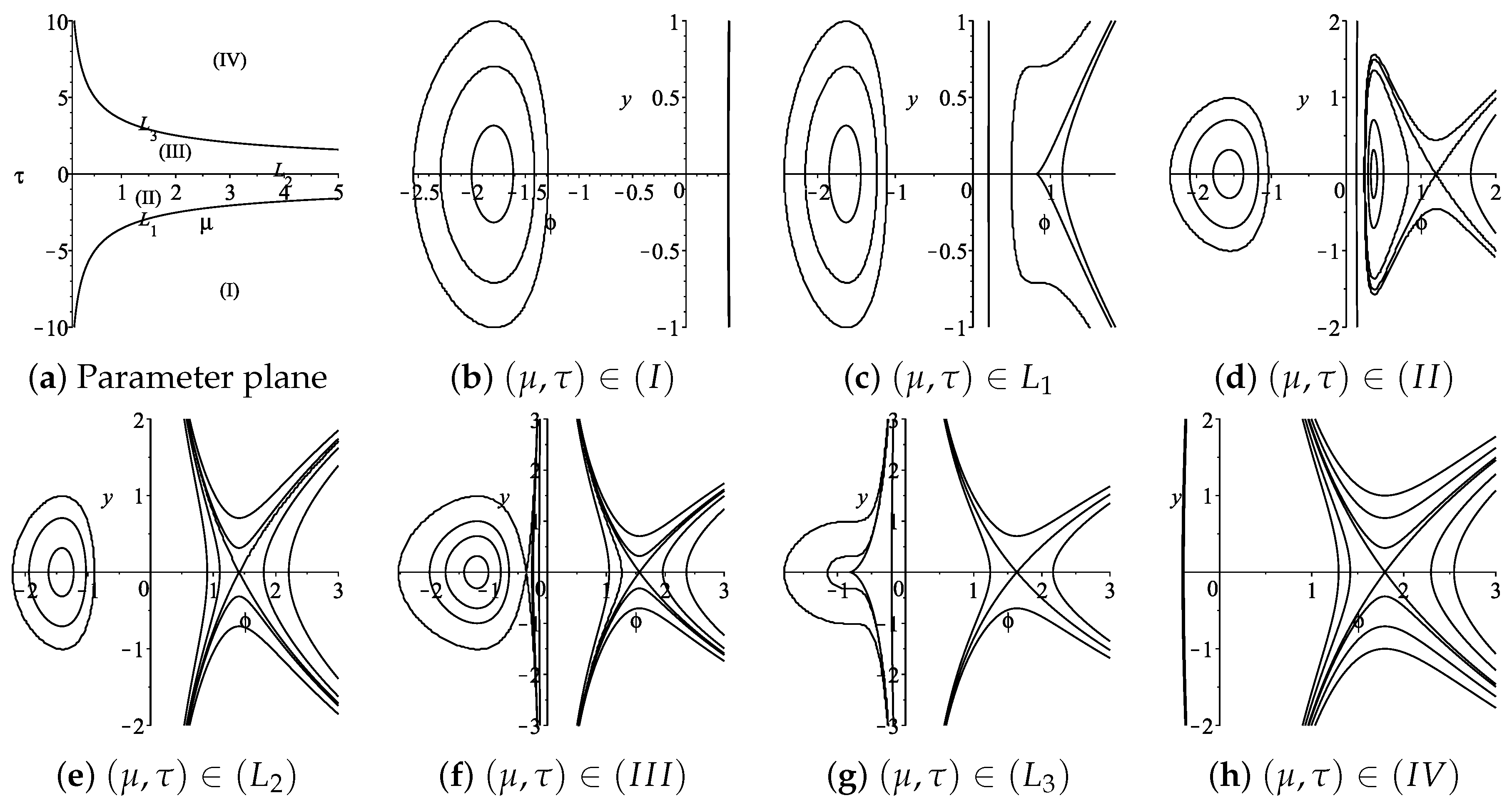
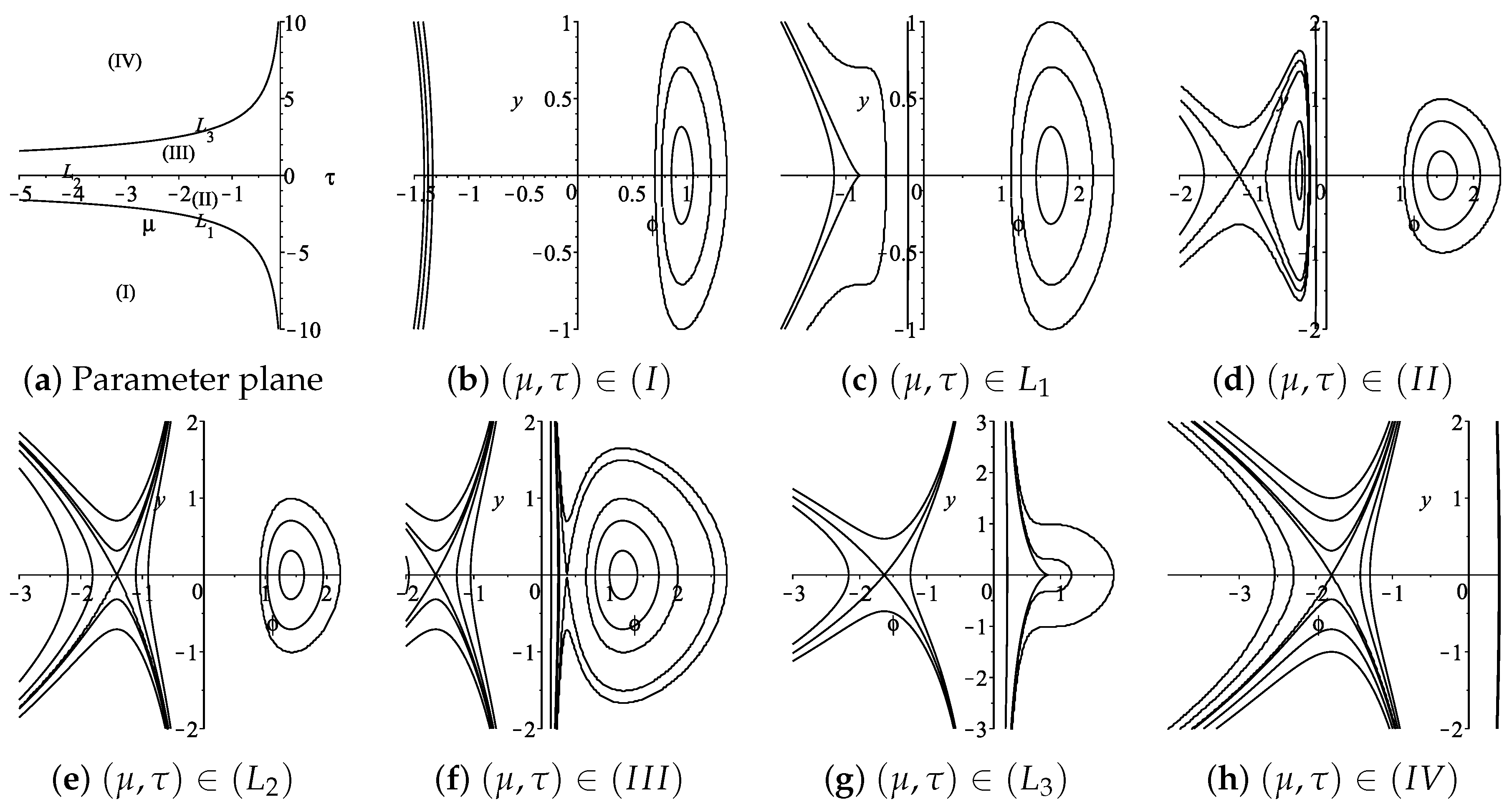
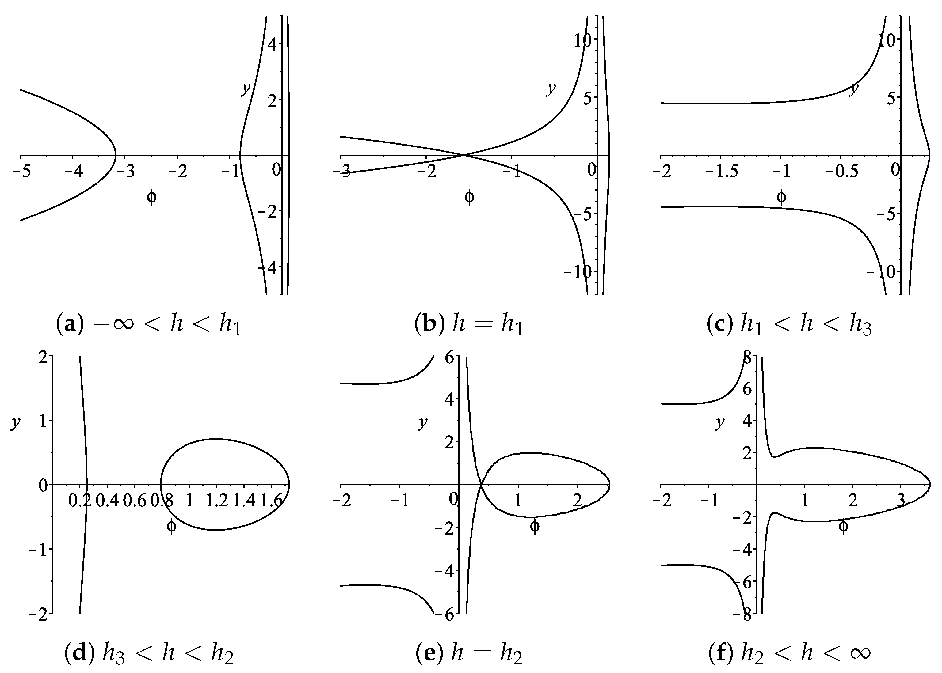
2. Bifurcation of Phase Portraits

We begin by considering all conceivable system (3) phase portraits. It is known that this system (3) has the same invariant curve solutions as the regular system it is connected with:

$$\frac{d\varphi }{d\zeta }=2y{\varphi }^3,\frac{dy}{d\zeta }=\mu {\varphi }^3-c\varphi -2\tau ,$$

(5)

where $d\xi =2{\varphi }^{3}d\zeta ,$ for $\varphi \ne 0$. We always assume that $\mu \ne 0.$

To study the equilibrium points of system (5), we write that $f\left(\varphi \right)={\varphi }^3-\frac{c}{\mu }\varphi -\frac{2\tau }{\mu },f^{\prime }\left(\varphi \right)=3{\varphi }^2-\frac{c}{\mu }.$ Obviously, if $c\mu >0,$ then, when $\varphi =\mp \widetilde{{\varphi }_0}={\left(\frac{c}{3\mu }\right)}^{\frac{1}{2}},f^{\prime }(\mp {\tilde{\varphi }}_0)=0.$ From $f(\mp {\tilde{\varphi }}_0)=0$ follow that $\tau =\mp \frac{\sqrt{3}}{9}\sqrt{\frac{c^3}{\mu }}.$ Thus, when $\tau <|\frac{\sqrt{3}}{9}\sqrt{\frac{c^3}{\mu }}|,$ function $f\left(\varphi \right)$ has three real simple zeros ${\varphi }_j,j=1,2,3$. Namely, on the $\varphi -$axis, system (5) has three equilibrium points $E_1({\varphi }_j,0),j=1,2,3.$ When $\tau =|\frac{\sqrt{3}}{9}\sqrt{\frac{c^3}{\mu }}|,$ function $f\left(\varphi \right)$ has a simple real zero and a double real zeros. When $\tau >|\frac{\sqrt{3}}{9}\sqrt{\frac{c^3}{\mu }}|,$ function $f\left(\varphi \right)$ has only one simple real zero.

For a fixed $c\ne 0,$ in $(\mu ,\tau )-$parameter plane, there exist three parameter curves

$$\left(L_1\right):\tau =-\frac{\sqrt{3}}{9}\sqrt{\frac{c^3}{\mu }},\left(L_2\right):\tau =0,\left(L_3\right):\tau =\frac{\sqrt{3}}{9}\sqrt{\frac{c^3}{\mu }},$$

which partition $(\mu ,\tau )-$parameter half-plane into four regions $\left(I\right)-\left(IV\right)$ (see Figure 1a and Figure 2a below).

Let $M({\varphi }_j,0)$ be the coefficient matrix of the linearized system of (5) at the equilibrium point $E_j({\varphi }_j,0)$. We have

$$J({\varphi }_j,0)=\det M({\varphi }_j,0)=-2{\varphi }_j^3(3\mu {\varphi }_j^2-c).$$

According to the theory of planar dynamical systems (see [4]), if $J<0$, then the equilibrium point is a saddle point. If $J>0$ and ${\left(\mathrm{Trace}M\right)}^2-4J<0(>0),$ then it is a center point (a node point); if $J=0$ and the Poincaré index of the equilibrium point is 0, then this equilibrium point is a cusp.

We write that $h_j=H_{(}{\varphi }_j,0),$ where H is given by (4).

By the above discussion, for a fixed parameter pair c, we have the bifurcations of phase portraits of system (3) shown in Figure 1 and Figure 2

We have the bifurcations of phase portraits of system (3) depicted in Figure 1 and Figure 2, as a result of the above explanation, for a fixed parameter pair c,

It is easy to see that the phase portraits in Figure 1 and Figure 2 are symmetrical with respect to the $y-$axis. Therefore, we next only need to consider one case for Figure 1 or Figure 2.

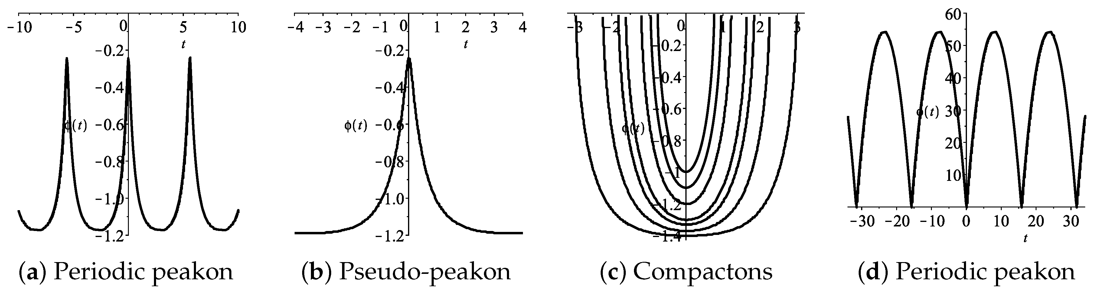
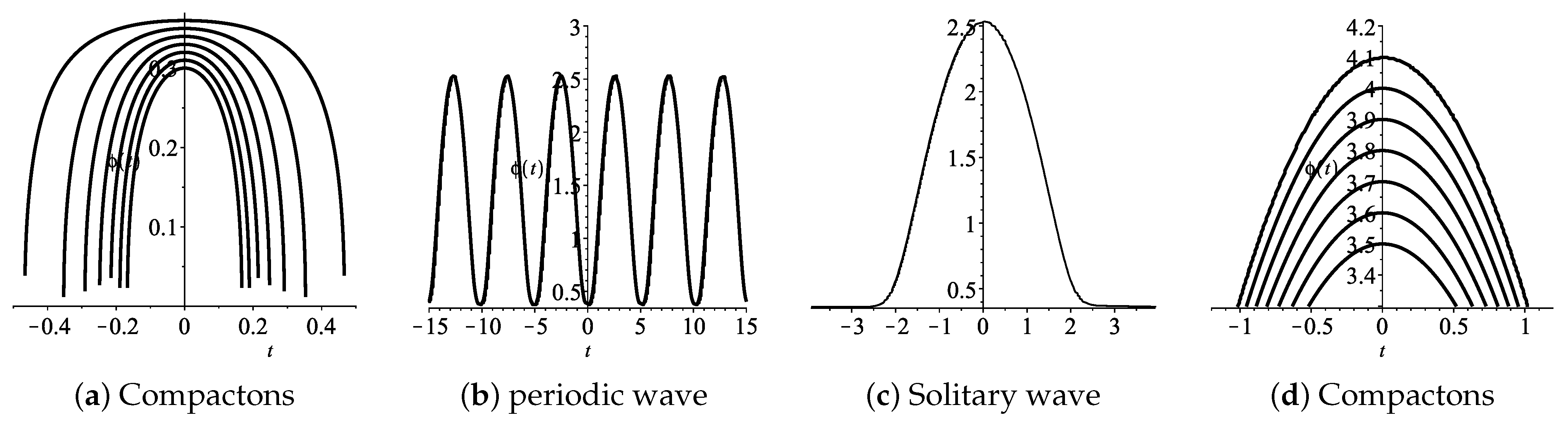
3. Exact Pseudo-Peakons, Periodic Peakons and Compactons Determined by the Orbits When $\mathit{c}<\mathbf{0},\mathit{\mu }<\mathbf{0}$

When $c<0,\mu <0$, we see from (4) that $y^2=\frac{\tau +c\varphi +h{\varphi }^2+\mu {\varphi }^3}{{\varphi }^2}.$ By using the first equation of (4), we obtain

$$\sqrt{\left|\mu \right|}\xi ={\int }_{{\varphi }_0}^{\varphi }\frac{\left|\varphi \right|d\varphi }{\sqrt{\frac{\tau }{\left|\mu \right|}+\frac{c}{\left|\mu \right|}\varphi +\frac{h}{\left|\mu \right|}{\varphi }^2-{\varphi }^3}}.$$

(6)

By using (6), we can obtain the parametric representations of all orbits defined by system (3).

3.1. $(\mu ,\tau )\in \left(I\right),\left(L_1\right)$: Exact Periodic Solution Family Defined by the Level Curves $H(\varphi ,y)=h,h\in (h_3,\infty )$

In this case, (6) can be written as $\sqrt{\left|\mu \right|}\xi ={\int }_{{\varphi }_b}^{\varphi }\frac{\varphi d\varphi }{\sqrt{({\varphi }_a-\varphi )(\varphi -{\varphi }_b)(\varphi -{\varphi }_c)}},$ where ${\varphi }_c<0<{\varphi }_b<{\varphi }_1<{\varphi }_a$. It gives rise to the following parametric representations of periodic family:

$$\begin{array}{cc}\varphi \left(\chi \right)\hfill & ={\varphi }_c+\frac{{\varphi }_b-{\varphi }_c}{{\mathrm{dn}}^2(\chi ,k)},\hfill \\ \xi \left(\chi \right)\hfill & =\sqrt{\frac{2}{\left|\mu \right|({\varphi }_a-{\varphi }_c)}}\left[{\varphi }_c\chi +({\varphi }_b-{\varphi }_c)\Pi (arcsin\left(\mathrm{sn}(\chi ,k)\right),\frac{{\varphi }_c}{{\varphi }_b},k)\right],\hfill \end{array}$$

(7)

where $k^2=\frac{{\varphi }_a-{\varphi }_b}{{\varphi }_a-{\varphi }_c},\mathrm{dn}(\chi ,k)$ is the Jacobian elliptic function, $\Pi (·,·,k)$ are elliptic integral of the third kind (see [12]).

Notice that because system (3) has a singular straight line $\varphi =0$, when ${\varphi }_b\ll 1$, (7) give rise to a periodic peakon family (see Figure 3d, below).

3.2. $(\mu ,\tau )\in \left(II\right)$: Two Exact Periodic Solution Families Defined by the Level Curves $H(\varphi ,y)=h,h\in (h_2,h_1),(h_3,\infty )$, Respectively, and a Pseudo-Peakon or Solitary Wave Solution Defined by $H(\varphi ,y)=h_1$

(i) For two families of periodic orbits defined by $H(\varphi ,y)=h$, when $h\in (h_2,h_1)$, we have ${\varphi }_c<{\varphi }_1<{\varphi }_b<{\varphi }_2<{\varphi }_a<0.$ When $h\in (h_3,\infty ),$ we have ${\varphi }_c<0<{\varphi }_b<{\varphi }_3<{\varphi }_a.$ They have the same parametric representations as (7).

(ii) For the homoclinic orbit to the equilibrium point $E_1({\varphi }_1,0)$ encosing the equilibrium point $E_2({\varphi }_2,0)$, (6) can be written as $\sqrt{\left|\mu \right|}\xi ={\int }_{\varphi }^{{\varphi }_M}\frac{\varphi d\varphi }{(\varphi -{\varphi }_1)\sqrt{({\varphi }_M-\varphi )}}.$ It gives rise to the following solitary wave solution:

$$\begin{array}{cc}\varphi \left(\chi \right)\hfill & ={\varphi }_M-({\varphi }_M-{\varphi }_1){tanh}^2\left(\frac{1}{2}\sqrt{{\varphi }_M-{\varphi }_1}\chi ,k\right),\hfill \\ \xi \left(\chi \right)\hfill & =\frac{1}{\sqrt{\left|\mu \right|}}\left[{\varphi }_1\chi \pm 2\sqrt{{\varphi }_M-\varphi \left(\chi \right)}\right],\chi \in (-\infty ,0),(0,\infty ),\mathrm{respectively}.\hfill \end{array}$$

(8)

When $|{\varphi }_M|\ll 1,$ (7) defined a family of periodic peakons (see Figure 3a). Equation (8) defined a pseudo-peakon solution (see Figure 3b).

3.3. $(\mu ,\tau )\in \left(L_2\right),\tau =0$: An Exact Compacton Solution Family Defined by $H(\varphi ,y)=h,h\in (-\infty ,h_1]$ and a Periodic Solution Family Defined by the Level Curves $H(\varphi ,y)=h,h\in (h_3,\infty )$

(i) Corresponding to the open level curves passing though the point $({\varphi }_b,0),{\varphi }_1<{\varphi }_b<0,$ defined by $H(\varphi ,y)=h,h\in (-\infty ,h_1)$, (6) can be written as $\sqrt{\left|\mu \right|}\xi ={\int }_{{\varphi }_b}^{\varphi }\frac{-\varphi d\varphi }{\sqrt{-\varphi (\varphi -{\varphi }_b)(\varphi -{\varphi }_c)}}.$ Thus, we obtain the following parametric representation of the compacton solution family (see Figure 3c):

$$\begin{array}{cc}\varphi \left(\chi \right)\hfill & ={\varphi }_c+\frac{{\varphi }_b-{\varphi }_c}{{\mathrm{dn}}^2(\chi ,k)},\chi \in (-{\chi }_{{}_{01}},{\chi }_{{}_{01}}),\hfill \\ \xi \left(\chi \right)\hfill & =\sqrt{\frac{2}{\left|\mu \right|(-{\varphi }_c)}}\left[{\varphi }_c\chi +({\varphi }_b-{\varphi }_c)\Pi (arcsin\left(\mathrm{sn}(\chi ,k)\right),\frac{{\varphi }_c}{{\varphi }_b},k)\right],\hfill \end{array}$$

(9)

where $k^2=\frac{{\varphi }_b}{{\varphi }_c},{\chi }_{{}_{01}}={\mathrm{dn}}^{-1}\left(\sqrt{\frac{-{\varphi }_c}{{\varphi }_b-{\varphi }_c}},k\right)$.

(ii) Corresponding to the right stable and unstable manifolds of the saddle point $E_1({\varphi }_1,0)$ defined by $H(\varphi ,y)=h_1,$ (6) can be written as $\sqrt{\left|\mu \right|}\xi =\pm {\int }_{\varphi }^0\frac{-\varphi d\varphi }{(\varphi -{\varphi }_1)\sqrt{-\varphi }}.$ It follows the parametric representations of two bounded solutions (see Figure 4a,b):

$$\begin{array}{cc}\varphi \left(\chi \right)\hfill & ={\varphi }_1{tanh}^2\left(\frac{1}{2}\sqrt{-{\varphi }_1}\chi \right),\chi \in (-\infty ,0),(0,\infty ),\mathrm{respectively},\hfill \\ \xi \left(\chi \right)\hfill & =\frac{1}{\sqrt{\left|\mu \right|}}\left[-{\varphi }_1\chi \pm 2\sqrt{-\varphi \left(\chi \right)}\right].\hfill \end{array}$$

(10)

Notice that if we take together the above two bounded solutions, then, we get a “cuspon solution” (see Figure 4c), which is not a correct solution. It consists of two solutions.

(iii) Corresponding to the closed level curve family, enclosing the point $E_3({\varphi }_3,0)$, defined by $H(\varphi ,y)=h,h\in (h_3,\infty )$, (6) becomes that $\sqrt{\left|\mu \right|}\xi ={\int }_{{\varphi }_b}^{\varphi }\frac{\varphi d\varphi }{\sqrt{({\varphi }_a-\varphi )(\varphi -{\varphi }_b)\varphi }}.$ Hence, we have the following parametric representation of periodic solution family:

$$\begin{array}{cc}\varphi \left(\chi \right)\hfill & =\frac{{\varphi }_b}{{\mathrm{dn}}^2(\chi ,k)},\hfill \\ \xi \left(\chi \right)\hfill & =\sqrt{\frac{2}{\left|\mu \right|{\varphi }_a}}\left[{\varphi }_{b}F(arcsin\left(\mathrm{sn}(\chi ,k)\right),k)\right],\hfill \end{array}$$

(11)

where $k^2=1-\frac{{\varphi }_b}{{\varphi }_a},F(·,k)$ is the normal elliptic integral of the first kind.

3.4. $(\mu ,\tau )\in \left(III\right)$: Two Exact Compacton Solution Families Defined by $H(\varphi ,y)=h,h\in (-\infty ,h_1]$ and a Periodic Solution Family Defined by the Level Curves $H(\varphi ,y)=h,h\in (h_3,h_2)$, et al.

When $(\mu ,\tau )\in \left(III\right)$, in Figure 2f, the changes of level curves defined by $H(\varphi ,y)=h$ are shown in Figure 5a–f.

(i) Corresponding to the two open level curve families passing though the point $({\varphi }_a,0)$ and $({\varphi }_b,0),{\varphi }_c<{\varphi }_1<{\varphi }_b<0<{\varphi }_a<{\varphi }_2,$ defined by $H(\varphi ,y)=h,h\in (-\infty ,h_1)$ (see Figure 5a), (6) can be written as $\sqrt{\left|\mu \right|}\xi ={\int }_{{\varphi }_b}^{\varphi }\frac{-\varphi d\varphi }{\sqrt{({\varphi }_a-\varphi )(\varphi -{\varphi }_b)(\varphi -{\varphi }_c)}}$ and $\sqrt{\left|\mu \right|}\xi ={\int }_{\varphi }^{{\varphi }_a}\frac{\varphi d\varphi }{\sqrt{({\varphi }_a-\varphi )(\varphi -{\varphi }_b)(\varphi -{\varphi }_c)}}.$

As a result, we get the parametric representations of the two compacton solution families as follows:

$$\begin{array}{cc}\varphi \left(\chi \right)\hfill & ={\varphi }_c+\frac{{\varphi }_b-{\varphi }_c}{{\mathrm{dn}}^2(\chi ,k)},\chi \in (-{\chi }_{{}_{01}},{\chi }_{{}_{01}}),\hfill \\ \xi \left(\chi \right)\hfill & =\sqrt{\frac{2}{\left|\mu \right|({\varphi }_a-{\varphi }_c)}}\left[{\varphi }_c\chi +({\varphi }_b-{\varphi }_c)\Pi (arcsin\left(\mathrm{sn}(\chi ,k)\right),\frac{{\varphi }_c}{{\varphi }_b},k)\right],\hfill \end{array}$$

(12)

where $k^2=\frac{{\varphi }_a-{\varphi }_b}{{\varphi }_a-{\varphi }_c},{\chi }_{{}_{01}}={\mathrm{dn}}^{-1}\left(\sqrt{\frac{-{\varphi }_c}{{\varphi }_b-{\varphi }_c}},k\right)$. And

$$\begin{array}{cc}\varphi \left(\chi \right)\hfill & ={\varphi }_a-({\varphi }_a-{\varphi }_b){\mathrm{sn}}^2(\chi ,k),\chi \in (-{\chi }_{{}_{02}},{\chi }_{{}_{02}}),\hfill \\ \xi \left(\chi \right)\hfill & =\sqrt{\frac{2}{\left|\mu \right|({\varphi }_a-{\varphi }_c)}}\left[{\varphi }_c\chi +({\varphi }_a-{\varphi }_c)E(arcsin\left(\mathrm{sn}(\chi ,k)\right),k)\right],\hfill \end{array}$$

(13)

where $k^2=\frac{{\varphi }_a-{\varphi }_b}{{\varphi }_a-{\varphi }_c},{\chi }_{{}_{02}}={\mathrm{sn}}^{-1}\left(\sqrt{\frac{{\varphi }_a}{{\varphi }_a-{\varphi }_b}},k\right)$.

(ii) Corresponding to the right stable and unstable manifolds of the saddle point $E_1({\varphi }_1,0)$ and a open curve passing through the point$({\varphi }_a,0),0<{\varphi }_a<{\varphi }_2,$ defined by $H(\varphi ,y)=h_1$ (see Figure 5b), (6) can be written as $\sqrt{\left|\mu \right|}\xi =\pm {\int }_{\varphi }^0\frac{-\varphi d\varphi }{(\varphi -{\varphi }_1)\sqrt{{\varphi }_a-\varphi }}$ and $\sqrt{\left|\mu \right|}\xi =\pm {\int }_{\varphi }^{{\varphi }_a}\frac{\varphi d\varphi }{(\varphi -{\varphi }_1)\sqrt{{\varphi }_a-\varphi }}.$

It follows the parametric representations of two bounded solutions (similar to Figure 4a,b):

$$\begin{array}{cc}\varphi \left(\chi \right)\hfill & ={\varphi }_a-({\varphi }_a-{\varphi }_1){tanh}^2\left(\frac{1}{2}\sqrt{{\varphi }_a-{\varphi }_1}\chi \right),\chi \in (-\infty ,-{\chi }_{{}_{03}}),({\chi }_{{}_{03}},\infty ),\mathrm{respectively},\hfill \\ \xi \left(\chi \right)\hfill & =\frac{1}{\sqrt{\left|\mu \right|}}\left[-{\varphi }_1\chi \pm 2\sqrt{{\varphi }_a-\varphi \left(\chi \right)}\pm {\xi }_{01}\right].\hfill \end{array}$$

(14)

where ${\chi }_{{}_{03}}=\frac{2}{\sqrt{{\varphi }_a-{\varphi }_1}}{tanh}^{-1}\sqrt{\frac{{\varphi }_a}{{\varphi }_a-{\varphi }_1}},{\xi }_{01}=2\sqrt{{\varphi }_a}-\frac{2{\varphi }_1}{\sqrt{{\varphi }_a-{\varphi }_1}}{tanh}^{-1}\sqrt{\frac{{\varphi }_a}{{\varphi }_a-{\varphi }_1}}$. We have a compactom solution as follows:

$$\begin{array}{cc}\varphi \left(\chi \right)\hfill & ={\varphi }_a-({\varphi }_a-{\varphi }_1){tanh}^2\left(\frac{1}{2}\sqrt{{\varphi }_a-{\varphi }_1}\chi \right),\chi \in (-{\chi }_{{}_{03}},0),(0,{\chi }_{{}_{03}}),\mathrm{respectively},\hfill \\ \xi \left(\chi \right)\hfill & =\frac{1}{\sqrt{\left|\mu \right|}}\left[{\varphi }_1\chi \mp 2\sqrt{{\varphi }_a-\varphi \left(\chi \right)}\right].\hfill \end{array}$$

(15)

(iii) Corresponding to the open curve family passing though the point $({\varphi }_a,0),0<{\varphi }_a<{\varphi }_2$ or ${\varphi }_2<{\varphi }_M<{\varphi }_a$, defined by $H(\varphi ,y)=h,h\in (h_3,h_2)$ or $h\in (h_2,\infty )$ (see Figure 5c,f), (6) can be written as $\sqrt{\left|\mu \right|}\xi ={\int }_{\varphi }^{{\varphi }_a}\frac{\varphi d\varphi }{\sqrt{({\varphi }_a-\varphi )[{(\varphi -b_1)}^2+a_1^2]}}.$ It gives rise to the following parametric representation of a compacton solution family (see Figure 6d):

$$\begin{array}{cc}\varphi \left(\chi \right)\hfill & =A_1+{\varphi }_a-\frac{2A_1}{1+\mathrm{cn}(\chi ,k)},\chi \in (-{\chi }_{{}_{04}},0),(0,{\chi }_{{}_{04}}),\mathrm{respectively},\hfill \\ \xi \left(\chi \right)\hfill & =\frac{1}{\sqrt{A_1\left|\mu \right|}}\left[({\varphi }_a+A_1)F(arcsin(\mathrm{sn}(\chi ,k),k)\mp 2-2A_1{\int }_0^{\chi }\frac{d\chi }{1+\mathrm{cn}(\chi ,k)}\right].\hfill \end{array}$$

(16)

where $A_1^2={(b_1-{\varphi }_a)}^2+a_1^2,k^2=\frac{A_1-b_1+{\varphi }_a}{2A_1},{\chi }_{{}_{04}}={\mathrm{cn}}^{-1}\sqrt{\frac{A_1-{\varphi }_a}{A_1+{\varphi }_a}}$.

(iv) Corresponding to the open curve family passing though the point $({\varphi }_c,0),0<{\varphi }_c<{\varphi }_2<{\varphi }_b<{\varphi }_3<{\varphi }_a,$ and the closed curve family enclosing the equilibrium point $E_3({\varphi }_3,0)$, defined by $H(\varphi ,y)=h,h\in (h_3,h_2)$ (see Figure 5d), (6) can be written as $\sqrt{\left|\mu \right|}\xi ={\int }_{\varphi }^{{\varphi }_c}\frac{\varphi d\varphi }{\sqrt{({\varphi }_a-\varphi )({\varphi }_b-\varphi )({\varphi }_c-\varphi )}}$ and $\sqrt{\left|\mu \right|}\xi ={\int }_{{\varphi }_b}^{\varphi }\frac{\varphi d\varphi }{\sqrt{({\varphi }_a-\varphi )(\varphi -{\varphi }_b)(\varphi -{\varphi }_c)}}.$ Hence, we obtain the following compacton solution family (see Figure 6a):

$$\begin{array}{cc}\varphi \left(\chi \right)\hfill & ={\varphi }_b-\frac{{\varphi }_b-{\varphi }_c}{{\mathrm{cn}}^2(\chi ,k)},\chi \in (-{\chi }_{{}_{05}},{\chi }_{{}_{05}}),\hfill \\ \xi \left(\chi \right)\hfill & =\sqrt{\frac{2}{\left|\mu \right|({\varphi }_a-{\varphi }_c)}}\left[{\varphi }_c\chi -\frac{({\varphi }_b+{\varphi }_c)}{1-k^2}\mathrm{dn}(\chi ,k)\mathrm{tn}(\chi ,k)+\frac{({\varphi }_b-{\varphi }_c)}{1-k^2}E(arcsin\left(\mathrm{sn}(\chi ,k)\right),k)\right],\hfill \end{array}$$

(17)

where $k^2=\frac{{\varphi }_a-{\varphi }_b}{{\varphi }_a-{\varphi }_c},{\chi }_{{}_{05}}={\mathrm{cn}}^{-1}\left(\sqrt{1-\frac{{\varphi }_c}{{\varphi }_b}},k\right)$.

The periodic family has the same parametric representation as (7) (see Figure 6b).

(v) Corresponding to the homoclinic orbit to the equilibrium point $E_2({\varphi }_2,0)$, passing though the point $({\varphi }_M,0),$ defined by $H(\varphi ,y)=h_2,$ (6) becomes that $\sqrt{\left|\mu \right|}\xi ={\int }_{\varphi }^{{\varphi }_M}\frac{\varphi d\varphi }{(\varphi -{\varphi }_2)\sqrt{{\varphi }_M-\varphi }}.$ Thus, we have the following solitary wave solution (see Figure 6c):

$$\begin{array}{cc}\varphi \left(\chi \right)\hfill & ={\varphi }_M-({\varphi }_M-{\varphi }_2){tanh}^2\left(\frac{1}{2}\sqrt{{\varphi }_M-{\varphi }_2}\chi ,k\right),\hfill \\ \xi \left(\chi \right)\hfill & =\frac{1}{\sqrt{\left|\mu \right|}}\left[{\varphi }_2\chi \mp 2\sqrt{{\varphi }_M-\varphi \left(\chi \right)}\right],\chi \in (-\infty ,0),(0,\infty ),\mathrm{respectively}.\hfill \end{array}$$

(18)

3.5. $(\mu ,\tau )\in \left(L_3\right)$: Exact Compacton Solution Families Defined by $H(\varphi ,y)=h,h\in (-\infty ,h_1),(h_1,h_2),(h_2,\infty )$, and Two Bounded Solutions Defined by the Level Curves $H(\varphi ,y)=h_2$

(i) In this parameter condition, all compacton families have the same parametric representations as the above cases.

(ii) Correspoding to the stable and unstable manifolds to the double equilibrium point $E_2({\varphi }_2,0)$ defined by $H(\varphi ,y)=h_2$, now, (6) has the form that $\pm \sqrt{\left|\mu \right|}\xi ={\int }_0^{\varphi }\frac{\varphi d\varphi }{{({\varphi }_2-\varphi )}^{\frac{3}{2}}}.$ Thus, the unstable manifold has the parametric representation:

$$\varphi \left(\xi \right)=\frac{1}{8}\left[2{\varphi }_2-{\left(4\sqrt{{\varphi }_2}-\sqrt{\left|\mu \right|}\xi \right)}^2+\left(4\sqrt{{\varphi }_2}-\sqrt{\left|\mu \right|}\xi \right)\sqrt{{\left(4\sqrt{{\varphi }_2}-\sqrt{\left|\mu \right|}\xi \right)}^2-16{\varphi }_2}\right].$$

(19)

The stable manifold has the parametric representation:

$$\varphi \left(\xi \right)=\frac{1}{8}\left[2{\varphi }_2-{\left(4\sqrt{{\varphi }_2}+\sqrt{\left|\mu \right|}\xi \right)}^2+\left(4\sqrt{{\varphi }_2}+\sqrt{\left|\mu \right|}\xi \right)\sqrt{{\left(4\sqrt{{\varphi }_2}+\sqrt{\left|\mu \right|}\xi \right)}^2-16{\varphi }_2}\right].$$

(20)

Notice that if we take together the above two bounded solutions, then we get a “anti-cuspon solution” (see Figure 7c), which is not a correct solution. It consists of two solutions.

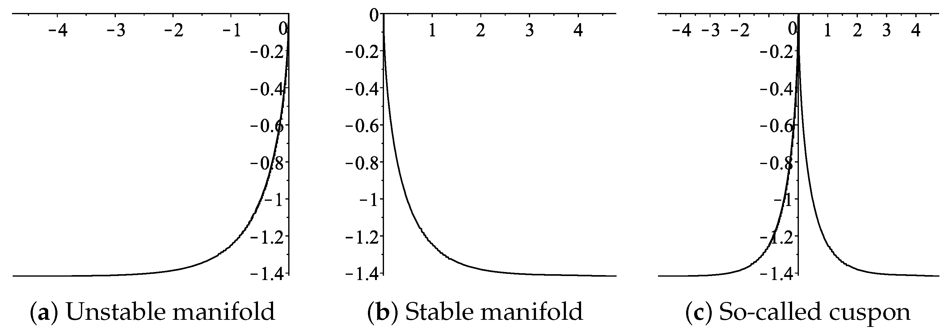
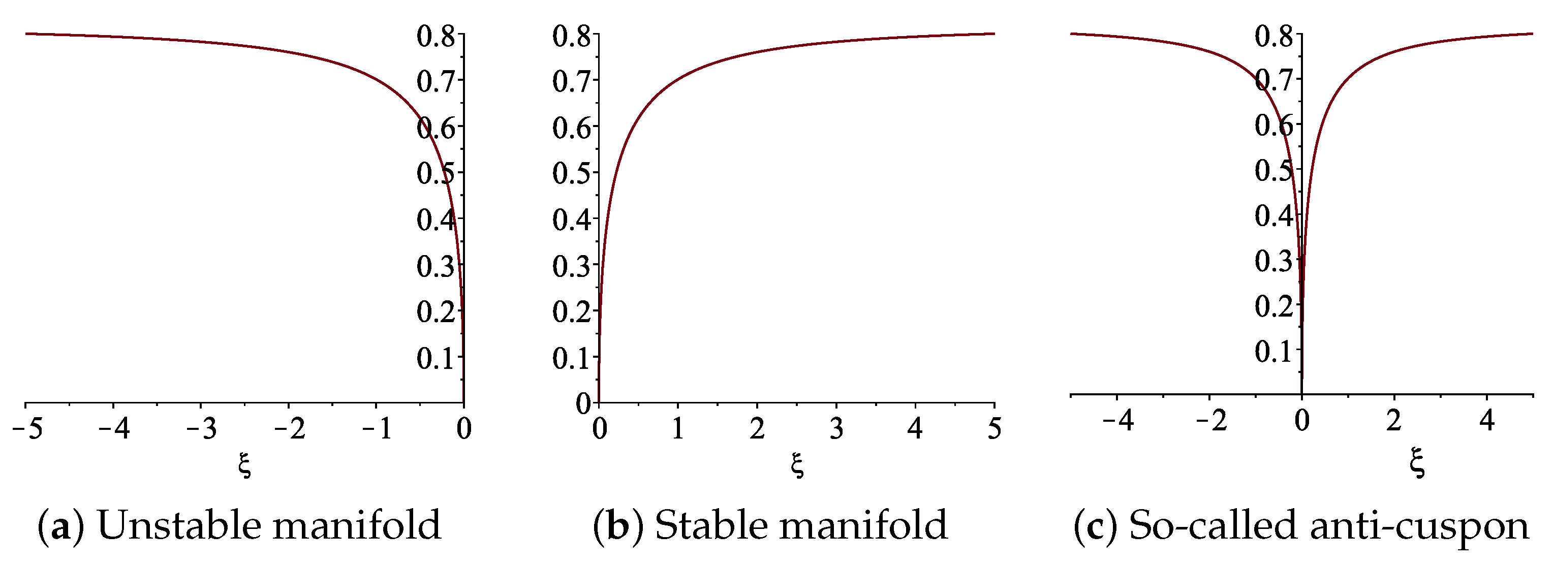
4. Exact Solitary Wave Solutions Determined by the Orbits When $\mathit{c}<\mathbf{0},\mathit{\mu }<\mathbf{0}$

In this section, we consider the exact solutions for Equation (1). Because we use the transformation $u(x,t)=\frac{1}{{\varphi }^2(x-ct)}$, such that Equation (1) becomes Equation (2), in order to study all solutions depending on parameters of system. Therefore, if a solution $\varphi \left(\xi \right)$ of system (3) can take some values which are near zero, then, $u(x-ct)$ becomes a unbounded solution. We do not like to consider the unbounded solution of Equation (1). By using the results of Section 3 we have the following conclusion.

Theorem 2.

For a fixed $c<0$ and $\mu <0,$ we have

(1) When $(\mu ,\tau )\in \left(II\right)$ in Figure 2a, Equation (1) has an exact solitary wave solution

$$\begin{array}{cc}u\left(\chi \right)\hfill & ={\left({\varphi }_M-({\varphi }_M-{\varphi }_1){tanh}^2\left(\frac{1}{2}\sqrt{{\varphi }_M-{\varphi }_1}\chi ,k\right)\right)}^{-2},\hfill \\ \xi \left(\chi \right)\hfill & =\frac{1}{\sqrt{\left|\mu \right|}}\left[{\varphi }_1\chi \pm 2\sqrt{{\varphi }_M-\varphi \left(\chi \right)}\right],\chi \in (-\infty ,0),(0,\infty ),\mathit{respectively}.\hfill \end{array}$$

(21)

(2) When $(\mu ,\tau )\in \left(III\right)$ in Figure 2a, Equation (1) has an exact solitary wave solution

$$\begin{array}{cc}u\left(\chi \right)\hfill & ={\left({\varphi }_M-({\varphi }_M-{\varphi }_2){tanh}^2\left(\frac{1}{2}\sqrt{{\varphi }_M-{\varphi }_2}\chi ,k\right)\right)}^{-2},\hfill \\ \xi \left(\chi \right)\hfill & =\frac{1}{\sqrt{\left|\mu \right|}}\left[{\varphi }_2\chi \mp 2\sqrt{{\varphi }_M-\varphi \left(\chi \right)}\right],\chi \in (-\infty ,0),(0,\infty ),\mathit{respectively}.\hfill \end{array}$$

(22)

For the periodic wave solutions of Equation (1), we can give similar results as Theorem 2. We omit them.

References

1. Camassa, R.; Holm, D.D. An integrable shallow water equation with peak solutions. Phys. Rev. Lett. 1993, 71, 1161–1164. [Google Scholar] [CrossRef] [PubMed] [Green Version]
2. Camassa, R.; Holm, D.D.; Hyman, J.M. A new integrable shallow water equation. Adv. Appl. Mech. 1994, 31, 1–33. [Google Scholar]
3. Camassa, R.; Hyman, J.M.; Luce, B.P. Nonlinear waves and solitons in physical sysytems. Physics D 1998, 123, 1–20. [Google Scholar] [CrossRef]
4. Li, J. Singular Nonlinear Traveling Wave Equations: Bifurcations and Exact Solutions; Science Press: Beijing, China, 2013. [Google Scholar]
5. Li, J.; Qiao, Z. Peakon, pseudo-peakon and cuspon solutions for two generalized Cammasa-Holm equations. J. Math. Phys. 2013, 54, 123501. [Google Scholar] [CrossRef] [Green Version]
6. Li, J.; Chen, G. On a class of singular nonlinear traveling wave equations. Int. J. Bifurc. Chaos 2007, 17, 4049–4065. [Google Scholar] [CrossRef]
7. Li, J.; Zhu, W.; Chen, G. Understanding peakons, periodic peakons and compactons via a shallow water wave equation. Int. J. Bifurc. Chaos 2016, 26, 1650207. [Google Scholar] [CrossRef]
8. Li, J. Variform exact one-peakon solutions for some singular nonlinear traveling wave equations of the first kind. Int. J. Bifurc. Chaos 2014, 24, 1450160. [Google Scholar] [CrossRef] [Green Version]
9. Geng, X.; Li, R.; Xue, B. A new integrable equation with peakons and cuspons and its bi-Hamiltonian structure. Appl. Math. Lett. 2015, 46, 64–69. [Google Scholar] [CrossRef]
10. Oono, H. N soliton solution of Harry Dym equation by inverse scattering method. In Nonlinear Physics: Theory and Experiment; World Scientific Publishing: River Edge, NJ, USA, 1996; pp. 241–248. [Google Scholar]
11. Fuchssteiner, B.; Schulze, T.; Carillo, S. Explicit solutions for the Harry Dym equation. J. Phys. A 1992, 25, 223–230. [Google Scholar] [CrossRef]
12. Byrd, P.F.; Fridman, M.D. Handbook of Elliptic Integrals for Engineers and Scientists; Springer: Berlin, Germany, 1971. [Google Scholar]
Figure 1. Bifurcations of phase portraits of system (3) for c > 0 , μ > 0 .
Symmetry 14 01480 g001
Figure 2. Bifurcations of phase portraits of system (3) for c < 0 , μ < 0 .
Symmetry 14 01480 g002
Figure 3. Profiles of periodic peakon, pseudo-peakon, and compactons.
Symmetry 14 01480 g003
Figure 4. Profiles of two bounded solutions and so-called cuspon solution.
Symmetry 14 01480 g004
Figure 5. Changes of level curves defined by H ( ϕ , y ) = h when ( μ , τ ) ( I I I ) .
Symmetry 14 01480 g005
Figure 6. Profiles of solitary wave, periodic wave, and compactons.
Symmetry 14 01480 g006
Figure 7. Profiles of two bounded solutions and so-called anti-cuspon solution.
Symmetry 14 01480 g007
Publisher’s Note: MDPI stays neutral with regard to jurisdictional claims in published maps and institutional affiliations.