A Hybrid RBF Collocation Method and Its Application in the Elastostatic Symmetric Problems

Abstract

In this paper, a new hybrid radial basis function collocation method (HRBF-CM) is proposed to help resolve two-dimensional elastostatic symmetric problems. In the new approach, the hybrid radial basis function (HRBF) combines the infinitely smooth RBF and piecewise smooth RBF, containing two parameters (the shape parameter and the weight parameter). Discretization schemes are presented in detail. We use MATLAB to implement the HRBF-CM and produce numerical results which demonstrate the potential of this method. The new method’s accuracy is higher than that of the traditional methods, especially in the case of a more significant number of nodes. We discuss the new method’s effectiveness compared to the widely used traditional RBF and also investigate the effect of parameters on the method’s performance under the new method.

1. Introduction

The radial basis function was proposed by Hardy in the 1970s [1] and has made outstanding contributions to surface fitting and solving interpolation problems. Several authors discretized the partial differential equations (PDEs) using the collocation method [2,3]. The RBF method has the following three advantages [4]: (i) it can be estimated without using a mesh; (ii) it is highly accurate; and (iii) it has sufficient flexibility in choosing basis functions. Generally, a radial function $\varphi \left(r_j\right)$ is a function of the Euclidean norm $r_j=\parallel x-x_j{\parallel }_2$, where $x\in {ℝ}^n$ is the center point and $x\in {ℝ}^n$ is a point in the influence domain of $x$.

Most radial basis functions can be divided into two categories (see some typical RBFs in

Table 1. Some typical RBFs.

Infinitely Smooth RBFs		Piecewise Smooth RBFs
Name	Expression	Name	Expression
Multiquadric (MQ)	$\sqrt{c^2+r_j^2}$	Splines of degree n (Sn)	$r_j^{2n-1},n\in \mathbb{N}$
Inverse multiquadric (IMQ)	$1/\sqrt{c^2+r_j^2}$	Thin plate spline (TPS)	$r_j^{2n}\log \left(r_j\right)$
Gaussian (GA)	$e^{-c^2{r}_j^2}$	Linear	$r_j$

Note: $r_j=\parallel x-x_j{\parallel }_2$, c represents the shape parameter.

). The first category uses infinitely smooth radial basis functions, including multiquadric (MQ), inverse multiquadric (IMQ), and Gaussian (EXP) functions. This type of radial basis function contains a shape parameter c, which needs to be defined by the user and controls the stability and accuracy of the RBF approximation. Therefore, choosing an optimal shape parameter value is imperative, which has also spurred discussion among many scholars. Generally, we prefer a constant optimal shape parameter (CSP) c throughout the computation, and the shape parameter c is the same for each node.

Some famous scholars proposed an experienced formula to select the optimal shape parameters [5,6,7]. Rippa chooses the best shape parameter c based on the minimization of the estimation of the error function and proposes the leave-one-out cross-validation (LOOCV) method [8]. However, it was assumed that CSP is not suitable. In this case, the approximation accuracy of the interpolation method was expected to be reduced, even more so than the approximation method of the general function, and the condition number of the matrix was large, resulting in an ill-conditioned linear system [9,10]. Kansa and Sarra used the variable shape parameter (VSP) form to solve this problem [11,12]. VSP is used to assign different values to the shape parameters which correspond to each center. This shows that each row of the RBF matrix has other shape parameters, which makes the condition number reduction in the RBF matrix more stable and improves the approximation of the interpolation function. Another method was used to determine the interval of the shape parameter, rather than a value, without any minimization and estimation error [13]. The purpose of VSP is to convert several CSPs into an interval range. Some other VSP strategies are summarized in [14,15,16].

It can be seen that choosing optimal shape parameter values in infinitely smooth RBFs is essential and has been an ongoing challenge. In contrast, the second set of piecewise smooth RBFs is not infinitely differentiable. They have no shape parameter and are easier to implement than the former group when used. However, they only lead to algebraic convergence rates and are rarely used alone in applications [17]. Therefore, many researchers prefer using infinitely smooth RBFs in scientific computing and engineering applications [18,19,20,21].

Some scholars bypassed the process of seeking optimal shape parameters and proposed a nontraditional RBF. For instance, Karimi [22] introduces a new Gaussian RBF (GRBF), which is both stable and accurate and is free of instability issues for small values of the shape parameter. Similarly, Zhang [17] proposed a new global RBF based on the coupling of infinitely smooth RBF with the conical spines, known as the coupled radial basis function (CRBF). He used the CRBF method in the Kansa method to produce a relatively good linear system. The condition number is moderate, and the error changes slightly with the change in the shape parameter value. Cao [23] uses this CRBF method to reconstruct the elasticity problem. However, there are still some deficiencies in the calculation accuracy, and the operation time is too long. Recently, Manzoor [24] used this similar idea to propose a hybrid radial basis function (HRBF) method, which combines two different RBFs: an infinite smooth RBF defined by shape parameters and a piecewise smooth RBF that is independent of shape parameters. This method has better accuracy when solving Burgers’ equations. In this paper, we use this method to solve elastostatic symmetric problems.

The predecessors have also made great efforts to solve elastostatic problems [25,26,27,28,29,30,31,32,33,34,35]. This paper mainly studies two well-known examples: cantilever beams and thin plates with circular holes. Zhang [25] applied the globally supported RBFs, i.e., MQ, IMQ, and Wendland’s functions [26]. Tolstykh and Shirobokov [27] applied the local RBF method. Liu et al. proposed a combination of Galerkin weak form and RBFs, namely the radial point interpolation method (RPIM) [28,29,30,31]. Simonenko [32] analyzes the applicability of both the global and the local versions of the method for elastostatic problems. They use multiquadric functions as RBFs and describe how to select an optimal shape parameter value to minimize approximation errors. Based on Simonenko’s article, we use the HRBF instead of MQ-RBF and the global Kansa method to conduct numerical experiments.

This paper is structured as follows. In Section 2, we first introduce the origin of the hybrid radial basis function, list the several types of HRBF, and describe the HRBF-CM’s formulation to find a solution to elastostatic problems. In Section 3, three numerical examples are calculated to verify the validity and accuracy of the HRBF collocation method, namely a patch test, a cantilever beam, and an infinite plate with a central hole. We compare the accuracy of the HRBF-CM with the infinitely smooth RBFs and the piecewise smooth RBFs. The distribution of two kinds of regular and irregular nodes is considered, and the influence of shape and weight parameters on the calculation results is discussed. The last section provides a summary of this method.

2. The HRBF-CM for Elastostatic Symmetric Problems

In this section, we describe the origin of the HRBF, the HRBF used in this article, and the process of solving elastostatic equations using the HRBF-CM in detail.

2.1. The Construction of HRBFs

As presented in [24], by coupling the infinite smoothing RBFs (${\varphi }_1$), such as MQ, IMQ, and GA, with the piecewise smooth RBFs Sn and TPS RBFs (${\varphi }_2$), the HRBF is constructed and can be defined as

$$R\left(r_j\right)=\gamma {\varphi }_1\left(r_j\right)+ϵ{\varphi }_2\left(r_j\right),\hspace{1em}{r}_j=\parallel x-x_j{\parallel }_2,$$

(1)

where the parameters $\gamma$ and $ϵ$ are positive real numbers that control the contributions of ${\varphi }_1$ and ${\varphi }_2$, respectively. ${\varphi }_1$ is an infinite smooth RBF with a user-defined shape parameter $c$, and ${\varphi }_2$ is a piecewise smooth RBF free from shape parameter.

Here, we find that the HRBF has three parameters, which seem to increase the algorithm’s complexity. At this point, we can scale the HRBF by a constant, which will not affect the algorithm. Therefore, the HRBF (1) can be normalized by the constant $w=ϵ/\gamma$ and has been redefined as

$$R_w\left(r_j\right)={\varphi }_1\left(r_j\right)+w{\varphi }_2\left(r_j\right).$$

(2)

Note that the reconstructed HRBF (2) now contains two parameters (the shape parameter c and the weight parameter $w$). These two parameters control the accuracy and stability of the HRBF-CM. The HRBFs to be used in this paper are listed in

Table 2. The hybrid RBFs.

Name	Expression
MQ + TPS	$\sqrt{r_j^2+c^2}+w{r}_j^4\ln \left(r_j\right)$
IMQ + TPS	$1/\sqrt{r_j^2+c^2}+w{r}_j^4\ln \left(r_j\right)$
GA + TPS	$e^{-c^2{r}_j^2}+w{r}_j^4\ln \left(r_j\right)$
MQ + S3	$\sqrt{r_j^2+c^2}+w{r}_j^3$
IMQ + S3	$1/\sqrt{r_j^2+c^2}+w{r}_j^3$
GA + S3	$e^{-c^2{r}_j^2}+w{r}_j^3$

Note: $r_j=\parallel x-x_j{\parallel }_2$, c represents the shape parameter, and w represents the weight parameter.

. It has been dictated in Mishra’s article [33] that a small value of the weight parameter $w$ usually gives acceptable accuracy with a stable spectrum (when all the eigenvalues of the differentiation matrix lie in the left half-plane). In Manzoor’s article [24], the authors calculated many numerical examples and concluded that in most of the test examples, for the three types of hybrid radial basis functions, MQ + S3, GS + S3, and IMQ + S3, the weight parameter w = 10⁻³ works best. On the other hand, for the three types of hybrid radial basis functions, MQ + TPS, GS + TPS, and IMQ + TPS, the weight parameter w = 10⁻⁹. However, in this work, we use w = [10⁰, 10⁻¹, 10⁻², 10⁻³, …, 10⁻¹⁵] to find the optimal parameter w.

2.2. The Elastostatic Equation

Considering the two-dimensional elastostatic symmetric problem, $\mathsf{\Omega }$ and $\Gamma$ represent the problem domain and the boundary, respectively. The equations of elasticity, written in terms of displacements, are defined as

$$\begin{array}{c}\frac{E}{1-{\mu }^2}\left(\frac{{\partial }^2{u}_x}{\partial x^2}+\frac{1-\mu }{2}\frac{{\partial }^2{u}_x}{\partial y^2}+\frac{1+\mu }{2}\frac{{\partial }^2{u}_y}{\partial x\partial y}\right)=f_x,\\ \frac{E}{1-{\mu }^2}\left(\frac{{\partial }^2{u}_y}{\partial y^2}+\frac{1-\mu }{2}\frac{{\partial }^2{u}_y}{\partial x^2}+\frac{1+\mu }{2}\frac{{\partial }^2{u}_x}{\partial x\partial y}\right)=f_y,\end{array} in \mathsf{\Omega }$$

(3)

with the displacement boundary condition

$$u_x={\overline{u}}_x,\hspace{1em}{u}_y={\overline{u}}_y,\hspace{1em}on\hspace{1em}{\Gamma }_u$$

(4)

and the stress boundary condition

$$\begin{array}{c}l{\sigma }_{xx}+m{\tau }_{xy}={\overline{t}}_x,\\ l{\tau }_{yx}+m{\sigma }_{yy}={\overline{t}}_y\end{array} on {\Gamma }_t$$

(5)

where u_x and u_y represent the displacement components on the boundary; f_x and f_y are the given body forces; $\overline{u}$ and $\overline{v}$ are the known functions of nodes on the displacement boundary ${\Gamma }_u$; l and m represent the cosine of the normal direction outside the slope; and ${\sigma }_{xx}, {\sigma }_{yy}, {\tau }_{xy}$ represent the stress constraints on the stress boundary ${\Gamma }_t$. E and $\mu$ stand for the Young’s modulus and the Poisson’s ratio, respectively. The stresses ${\sigma }_{xx}$, ${\sigma }_{yy}$, and ${\tau }_{xy}$ and the displacements u_x and u_y present the following relationship.

$$\{\begin{array}{l}{\sigma }_{xx}=\frac{E}{1-{\mu }^2}\left(\frac{\partial u_x}{\partial x}+\mu \frac{\partial u_y}{\partial y}\right),\hfill \\ {\sigma }_{yy}=\frac{E}{1-{\mu }^2}\left(\mu \frac{\partial u_x}{\partial x}+\frac{\partial u_y}{\partial y}\right),\hfill \\ {\tau }_{xy}=\frac{E}{2\left(1+\mu \right)}\left(\frac{\partial u_x}{\partial y}+\frac{\partial u_y}{\partial x}\right).\hfill \end{array}$$

(6)

2.3. The HRBF Formulation

Assuming that there are N distinct nodes ${\left\{x_i\right\}}_{i=1}^N$, the HRBF-CM is used to solve the elastostatic symmetric problem (3)–(5). In the HRBF-CM, the displacement approximate solutions $u_x\left(x\right)$ and $u_y\left(x\right)$ are separately spanned by a set of translated HRBFs, i.e.,

$$\{\begin{array}{l}{u}_x\left(x\right)={\displaystyle {\displaystyle \sum }_{j=1}^N}{a}_j{R}_w\left(r_j\right),\hfill \\ u_y\left(x\right)={\displaystyle {\displaystyle \sum }_{j=1}^N}{b}_j{R}_w\left(r_j\right).\hfill \end{array}$$

(7)

$R_w\left(r_j\right)$ with $r_j=\parallel x-x_j{\parallel }_2$ is the HRBF defined in Table 2. The unknown coefficients, a_j and b_j, are computed by a collocation of Equation (3) at a set of interior nodes and a collocation of the boundary conditions at boundary nodes. Let $z$ be defined as a vector of length 2N containing the unknowns.

$$\{\begin{array}{l}{z}_j=a_j\hfill \\ z_{j+N}=b_j,\hfill \end{array}\hspace{1em}j=1,\dots ,N,$$

(8)

Then, a vector $f$ is defined,

$$\{\begin{array}{l}{f}_j=f_x\left(x_j\right)\hfill \\ f_{j+N}=f_y\left(x_j\right)\hfill \end{array}\hspace{1em}j=1,\dots ,N.$$

(9)

By substituting Equation (7) into the elastostatic Equation (3) and boundary conditions (4)–(5), we obtain the following linear system:

$$Gz=f.$$

(10)

For i = 1, …, N, the elements of j internal nodes corresponding to the matrix $G$ are

$$\{\begin{array}{c}{G}_{i,j\left(i\ne j\right)}=\frac{E}{1-{\mu }^2}\left[\frac{{\partial }^2{R}_w\left(r_{i,j}\right)}{\partial x^2}+\frac{1-\mu }{2}\frac{{\partial }^2{R}_w\left(r_{i,j}\right)}{\partial y^2}\right],\\ G_{i,j\left(i=j\right)}=\frac{E}{1-{\mu }^2}\left[\frac{{\partial }^2\varphi \left(r_{i,j}\right)}{\partial x^2}+\frac{1-\mu }{2}\frac{{\partial }^2\varphi \left(r_{i,j}\right)}{\partial y^2}\right].\end{array}$$

(11)

$$\{\begin{array}{c}{G}_{i,j+N\left(i\ne j+N\right)}=\frac{E}{2\left(1-\mu \right)}\frac{{\partial }^2{R}_w\left(r_{i,j}\right)}{\partial x\partial y},\\ G_{i,j+N\left(i=j+N\right)}=\frac{E}{2\left(1-\mu \right)}\frac{{\partial }^2\varphi \left(r_{i,j}\right)}{\partial x\partial y}. \end{array}$$

(12)

$$\{\begin{array}{c}{G}_{i+N,j\left(i+N\ne j\right)}=\frac{E}{2\left(1-\mu \right)}\frac{{\partial }^2{R}_w\left(r_{i,j}\right)}{\partial x\partial y},\\ G_{i+N,j\left(i+N=j\right)}=\frac{E}{2\left(1-\mu \right)}\frac{{\partial }^2\varphi \left(r_{i,j}\right)}{\partial x\partial y}. \end{array}$$

(13)

$$\{\begin{array}{c}{G}_{i+N,j\left(i+N\ne j+N\right)}=\frac{E}{1-{\mu }^2}\left[\frac{{\partial }^2{R}_w\left(r_{i,j}\right)}{\partial y^2}+\frac{1-\mu }{2}\frac{{\partial }^2{R}_w\left(r_{i,j}\right)}{\partial x^2}\right],\\ G_{i+N,j\left(i+N=j+N\right)}=\frac{E}{1-{\mu }^2}\left[\frac{{\partial }^2\varphi \left(r_{i,j}\right)}{\partial y^2}+\frac{1-\mu }{2}\frac{{\partial }^2\varphi \left(r_{i,j}\right)}{\partial x^2}\right].\end{array}$$

(14)

The elements of the boundary nodes of the matrix $G$ depend on the boundary conditions. For instance, in the case of Dirichlet boundary conditions,

$$\{\begin{array}{c}{G}_{i,j}=R_w\left(r_{i,j}\right),\hspace{1em}{f}_j={\overline{u}}_x\left(x_j\right), \\ G_{i+N,j+N}=R_w\left(r_{i,j}\right),f_{j+N}={\overline{u}}_y\left(x_j\right), \end{array}$$

(15)

where ${\overline{u}}_x$ and ${\overline{u}}_y$ are the exact solutions of problem (3), and Equation (10) can be written as

$$\left(\begin{array}{cc}{G}_{i,j}& G_{i,j+N}\\ G_{i+N,j}& G_{i+N,j+N}\end{array}\right)\left(\begin{array}{l}{a}_j\hfill \\ b_j\hfill \end{array}\right)=\left(\begin{array}{l}{\overline{u}}_x\left(x_j\right)\hfill \\ {\overline{u}}_y\left(x_j\right)\hfill \end{array}\right).$$

(16)

Therefore, the coefficients a_j and b_j of Equation (7) are used to compute the horizontal and vertical displacements u_x and u_y, respectively. In addition, the stresses are computed from Equation (5) with

$$\frac{\partial u_x}{\partial x}={\displaystyle \sum }_{i=1}^N{a}_j\frac{\partial R_w\left(r_j\right)}{\partial x},$$

(17)

$$\frac{\partial u_x}{\partial y}={\displaystyle \sum }_{i=1}^N{a}_j\frac{\partial R_w\left(r_j\right)}{\partial y},$$

(18)

$$\frac{\partial u_y}{\partial x}={\displaystyle \sum }_{i=1}^N{b}_j\frac{\partial R_w\left(r_j\right)}{\partial x},$$

(19)

$$\frac{\partial u_y}{\partial y}={\displaystyle \sum }_{i=1}^N{b}_j\frac{\partial R_w\left(r_j\right)}{\partial y}.$$

(20)

3. Numerical Examples

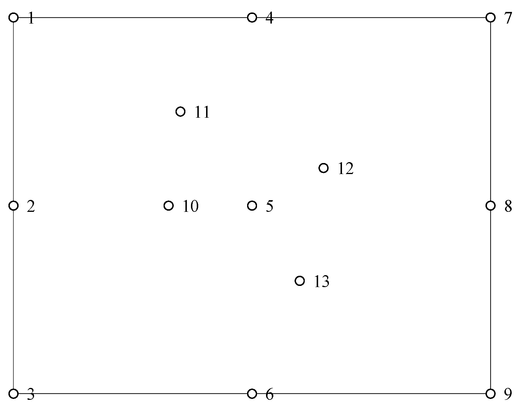
In this section, we use three numerical examples to verify the validity and the applicability of the hybrid radial basis function collocation method. The numerical results for these examples are compared with the analytical solutions and the traditional RBF solutions. The effect of different basis functions on computational accuracy is discussed.

To judge the validity and accuracy of the HRBF-CM method, we need a measure which can be measured by the relative error concerning the displacement and the stress:

$$\{\begin{array}{c}{r}_u=\sqrt{{\displaystyle {\displaystyle \sum }_{i=1}^N}{\left(u_i^{num}-u_i^{anal}\right)}^2}/\sqrt{{\displaystyle {\displaystyle \sum }_{i=1}^N}{u}_i^{{anal}^2}}\\ r_{\sigma }=\sqrt{{\displaystyle {\displaystyle \sum }_{i=1}^N}{\left({\sigma }_i^{num}-{\sigma }_i^{anal}\right)}^2}/\sqrt{{\displaystyle {\displaystyle \sum }_{i=1}^N}{\sigma }_i^{{anal}^2}}\end{array}$$

(21)

where $u_i^{num}$ and ${\sigma }_i^{num}$ are the numerical solutions for the displacement and stress of the ith node, respectively, and $u_i^{anal}$ and ${\sigma }_i^{anal}$ are the corresponding analytical solutions for the ith node.

3.1. Patch Test

The first numerical example is the standard patch test containing 13 nodes, with 5 irregular interior nodes, as shown in Figure 1. In this patch test, the essential boundary is the linear displacement assigned along the boundary. The linear displacement functions are u_x = 0.6x and u_y = 0.6y. Satisfying the patch test requires the same linear function to give the displacement of any interior node and requires the strains and stresses to be constant in the patch. In this problem, we randomly choose the shape parameter c = 1, the weight parameter referring to Manzoor’s article [24], the variant related to TPS, the weight parameter w = 10⁻⁹, the variant associated with S3, and the weight parameter w = 10⁻³. The HRBF passes the patch test with precision, as well as the traditional RBF. Different radial basis functions have different accuracies. The exact results of the internal node calculations for the MQ-HRBF and the traditional MQ-RBF are shown in

Table 3. Example 1: computational results of different methods (MQ and its variants).

Internal Node	Coordinates	Method
		Exact	MQ	MQ + TPS	MQ + S3
5	(1,1)
	(ux, uy)	(0.600,0.600)	(0.593,0.589)	(0.593,0.589)	(0.593,0.590)
	$\left({\sigma }_{xx},{\sigma }_{yy},{\tau }_{xy}\right)$	(0.857,0.857,0)	(0.896,0.890,0.010)	(0.896,0.890,0.010)	(0.895,0.889,0.010)
10	(0.65,1)
	(ux, uy)	(0.390,0.600)	(0.374,0.588)	(0.374,0.588)	(0.374,0.588)
	$\left({\sigma }_{xx},{\sigma }_{yy},{\tau }_{xy}\right)$	(0.857,0.857,0)	(0.893,0.900,0.009)	(0.893,0.900,0.009)	(0.892,0.899,0.009)
11	(0.7,1.5)
	(ux, uy)	(0.420,0.900)	(0.409,0.901)	(0.409,0.901)	(0.409,0.901)
	$\left({\sigma }_{xx},{\sigma }_{yy},{\tau }_{xy}\right)$	(0.857,0.857,0)	(0.906,0.893,−0.006)	(0.906,0.893,−0.006)	(0.904,0.892,−0.006)
12	(1.3,1.2)
	(ux, uy)	(0.780,0.720)	(0.784,0.718)	(0.784,0.718)	(0.784,0.718)
	$\left({\sigma }_{xx},{\sigma }_{yy},{\tau }_{xy}\right)$	(0.857,0.857,0)	(0.892,0.896,0.012)	(0.892,0.896,0.012)	(0.891,0.895,0.011)
13	(1.2,0.6)
	(ux, uy)	(0.720,0.360)	(0.718,0.343)	(0.718,0.343)	(0.718,0.343)
	$\left({\sigma }_{xx},{\sigma }_{yy},{\tau }_{xy}\right)$	(0.857,0.857,0)	(0.909,0.889,−0.003)	(0.909,0.889,−0.003)	(0.908,0.888,−0.003)

when the parameters are taken as E = 1 and v = 0.3.

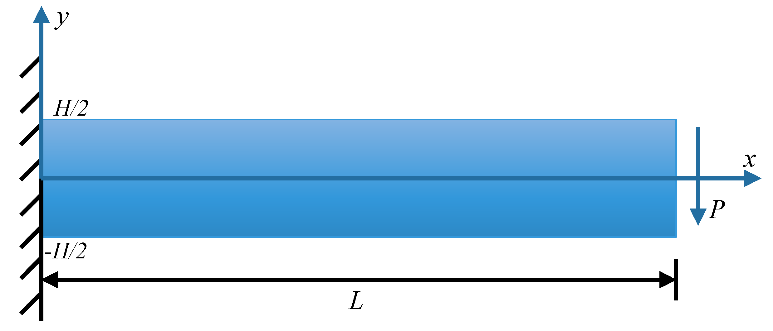
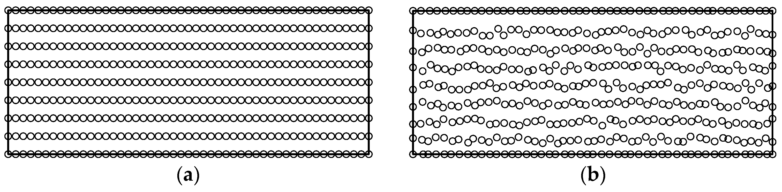
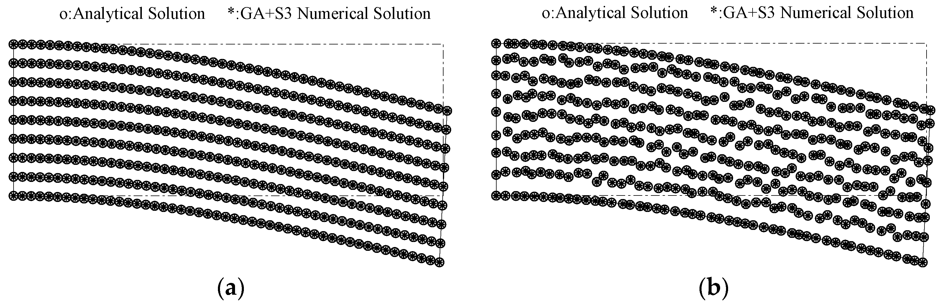
3.2. Cantilever Beam

For the second example, we consider a cantilever beam problem, as presented in Figure 2. A beam of length L and height H subjected to traction at the free end is considered. The beam has a unit thickness; hence, a plane stress problem is also considered here. The closed-form solution is available for the parabolic traction of force P:

$$\{\begin{array}{l}{u}_x^{anal}=-\frac{P}{6EI}\left(y-\frac{H}{2}\right)\left[\left(6L-3x\right)x+\left(2+\mu \right)\left(y^2-Hy\right)\right],\hfill \\ u_y^{anal}=\frac{P}{6EI}\left[3\mu {\left(y-\frac{H}{2}\right)}^2\left(L-x\right)+\left(4+5\mu \right)\frac{H^{2}x}{4}+\left(3L-x\right)x^2\right],\hfill \end{array}$$

(22)

where the moment of inertia I of the beam is given as I = H³/12.

The stresses corresponding to the above displacements are

$$\{\begin{array}{l}{\sigma }_{xx}^{anal}=-\frac{P\left(L-x\right)}{I}\left(y-\frac{H}{2}\right),\hfill \\ {\sigma }_{yy}^{anal}=0,\hfill \\ {\tau }_{xy}^{anal}=-\frac{P}{2I}\left(y^2-Hy\right).\hfill \end{array}$$

(23)

We refer to the study by Simonenko et al. [32] which uses the Dirichlet boundary conditions given by (22) in all the boundaries of the beam. The relevant parameters are L = 12; H = 2; E = 1000; μ = 0.3; p = −10.

3.2.1. Effect of Irregular Node Distribution

To investigate the stability of the HRBF-CM and its comparison with the traditional radial basis function method, both regular and irregular node distributions are used. Four kinds of regular node distributions, i.e., 13 × 3 (13 nodes in the x direction, 3 nodes in the $y$ direction), 25 × 5, 49 × 9, and 73 × 13, are considered. Four irregular distributions are used with the same number of nodes, i.e., 39, 125, 441, and 949. We discuss the effect of the node distributions on the numerical accuracy, and the results of the calculations are presented in

Table 4. Example 2: computational results of different methods for the irregular node distribution.

Method		N = 39	N = 125	N = 441	N = 949
MQ	copt	20	10	3	1.6
	ru	2.5513 × 10−6	7.1523 × 10−7	2.5843 × 10−7	3.7019 × 10−7
	$r_{\sigma }$	1.4577 × 10−3	8.6395 × 10−5	1.7324 × 10−4	3.3451 × 10−4
	CPU (s)	0.0445	0.0451	0.2092	0.7934
IMQ	copt	18	9	3	1.7
	ru	2.6001 × 10−6	9.4806 × 10−7	9.5554 × 10−7	2.6342 × 10−6
	$r_{\sigma }$	1.9224 × 10−3	6.2694 × 10−4	6.7735 × 10−4	2.4746 × 10−3
	CPU (s)	0.0270	0.0381	0.2288	0.9858
GA	copt	14.5	6.5	9	4.5
	ru	2.7955 × 10−6	4.1935 × 10−7	5.3383 × 10−6	3.8875 × 10−6
	$r_{\sigma }$	1.2317 × 10−3	5.5071 × 10−5	2.3780 × 10−4	1.9450 × 10−4
	CPU (s)	0.0071	0.0269	0.1128	0.4085
MQ + TPS	copt	(19.5,10−15)	(14,10−13)	(12.5,10−11)	(11.5,10−10)
	ru	3.3220 × 10−6	2.2796 × 10−7	2.1210 × 10−8	1.3474 × 10−8
	$r_{\sigma }$	2.8319 × 10−3	7.7843 × 10−5	9.3717 × 10−6	8.6273 × 10−6
	CPU (s)	0.0114	0.0723	0.2271	1.0846
IMQ + TPS	copt	(19,10−15)	(13,10−15)	(16,10−13)	(11.5,10−12)
	ru	2.2627 × 10−6	3.4743 × 10−7	4.7540 × 10−8	2.9863 × 10−8
	$r_{\sigma }$	1.6277 × 10−3	1.6833 × 10−4	2.8371 × 10−5	2.0773 × 10−5
	CPU (s)	0.0108	0.0396	0.2762	1.3265
GA + TPS	copt	(19.5,10−15)	(9.5,10−14)	(10,10−12)	(9,10−11)
	ru	2.7870 × 10−6	1.7480 × 10−7	3.5633 × 10−8	2.7927 × 10−8
	$r_{\sigma }$	1.5181 × 10−3	8.5198 × 10−5	2.1890 × 10−5	2.1679 × 10−5
	CPU (s)	0.0093	0.0686	0.2068	0.9901
MQ + S3	copt	(20,10−12)	(13,10−15)	(10,10−11)	(4.5,10−10)
	ru	5.1602 × 10−6	3.3904 × 10−7	4.5543 × 10−8	5.0247 × 10−8
	$r_{\sigma }$	2.8665 × 10−3	3.0302 × 10−5	2.1685 × 10−5	2.5899 × 10−5
	CPU (s)	0.0198	0.0585	0.1982	0.8878
IMQ + S3	copt	(20,10−15)	(13,10−15)	(14,10−13)	(15.5,10−13)
	ru	2.6737 × 10−6	1.3149 × 10−7	1.9911 × 10−8	1.1097 × 10−8
	$r_{\sigma }$	1.7319 × 10−3	5.7103 × 10−5	1.0639 × 10−5	5.6919 × 10−6
	CPU (s)	0.0127	0.0654	0.2489	1.1624
GA + S3	copt	(20,10−12)	(11,10−14)	(10.5,10−12)	(9,10−11)
	ru	3.0658 × 10−6	1.1867 × 10−7	1.3768 × 10−8	1.3672 × 10−8
	$r_{\sigma }$	2.9404 × 10−3	3.4692 × 10−5	9.9027 × 10−6	1.0190 × 10−5
	CPU (s)	0.0118	0.0573	0.1818	0.7992
TPS	ru	2.0007 × 10−4	7.5755 × 10−5	1.6952 × 10−5	8.0060 × 10−6
	$r_{\sigma }$	1.3620 × 10−1	2.7900 × 10−2	6.6000 × 10−3	2.9000 × 10−3
	CPU (s)	0.0051	0.0297	0.1314	0.5920
S3	ru	3.3979 × 10−4	1.8154 × 10−4	5.0393 × 10−5	2.7450 × 10−5
	$r_{\sigma }$	2.0560 × 10−1	8.5200 × 10−2	3.0800 × 10−2	1.7500 × 10−2
	CPU (s)	0.0279	0.0224	0.0978	0.4239

Note: The bold numbers represent the best calculated data.

and

Table 5. Example 2: computational results of different methods for regular node distribution.

Method		N =39 (3 × 13)	N =125 (5 × 25)	N =441 (9 × 49)	N =949 (13 × 73)
MQ	copt	18	14	3.5	1.7
	ru	8.0866 × 10−6	2.9725 × 10−6	4.0491 × 10−7	5.3096 × 10−7
	$r_{\sigma }$	8.3123 × 10−2	6.4158 × 10−4	1.2788 × 10−4	3.8119 × 10−4
	CPU (s)	0.0338	0.0437	0.1869	0.7948
IMQ	copt	18.5	16.5	3.5	2.1
	ru	1.2985 × 10−5	2.1955 × 10−6	1.4602 × 10−6	1.1814 × 10−6
	$r_{\sigma }$	8.0496 × 10−2	6.9578 × 10−4	6.7189 × 10−4	7.5492 × 10−4
	CPU (s)	0.0852	0.0390	0.2182	0.9871
GA	copt	18	13	4	6
	ru	7.3142 × 10−6	2.5473 × 10−6	3.7281 × 10−6	5.8424 × 10−6
	$r_{\sigma }$	6.1412 × 10−2	3.6249 × 10−4	2.1470 × 10−4	2.2683 × 10−4
	CPU (s)	0.0073	0.0237	0.2114	0.4151
MQ + TPS	copt	(20,10−15)	(20,10−10)	(11,10−11)	(10.5,10−10)
	ru	7.1497 × 10−6	7.4186 × 10−7	1.4188 × 10−8	9.3300 × 10−9
	$r_{\sigma }$	8.5075 × 10−2	2.9660 × 10−4	8.1700 × 10−6	6.4800 × 10−6
	CPU (s)	0.0467	0.0572	0.2321	1.0553
IMQ + TPS	copt	(20,10−15)	(20,10−14)	(11.5,10−13)	(10.5,10−12)
	ru	1.2108 × 10−5	1.2125 × 10−6	2.9799 × 10−8	1.5791 × 10−8
	$r_{\sigma }$	7.6433 × 10−2	4.5468 × 10−4	2.1833 × 10−5	1.5639 × 10−5
	CPU (s)	0.0444	0.0696	0.2802	1.3881
GA + TPS	copt	(20,10−10)	(20,10−13)	(10,10−12)	(9,10−11)
	ru	3.4546 × 10−6	3.7997 × 10−7	2.6746 × 10−8	2.0292 × 10−8
	$r_{\sigma }$	5.8012 × 10−2	1.5217 × 10−4	1.9862 × 10−5	1.6821 × 10−5
	CPU (s)	0.0069	0.0319	0.2191	0.9833
MQ + S3	copt	(1910−12)	(20,10−12)	(11,10−11)	(9,10−10)
	ru	5.3438 × 10−6	7.6381 × 10−7	3.1988 × 10−8	2.9318 × 10−8
	$r_{\sigma }$	7.5212 × 10−2	2.7886 × 10−4	1.8097 × 10−5	3.0168 × 10−5
	CPU (s)	0.0398	0.0329	0.2059	0.8991
IMQ + S3	copt	(20,10−15)	(20,10−13)	(14.5,10−13)	(16,10−13)
	ru	1.3095 × 10−5	1.1944 × 10−6	1.2919 × 10−8	6.9444 × 10−9
	$r_{\sigma }$	7.7167 × 10−2	4.3883 × 10−4	8.8861 × 10−6	4.4397 × 10−6
	CPU (s)	0.0309	0.0372	0.2585	1.1514
GA + S3	copt	(20,10−12)	(20,10−13)	(11,10−12)	(9.5,10−11)
	ru	4.5154 × 10−6	3.4575 × 10−7	1.2244 × 10−8	9.7053 × 10−9
	$r_{\sigma }$	5.8101 × 10−2	1.2654 × 10−4	8.6607 × 10−6	8.6815 × 10−6
	CPU (s)	0.0053	0.0297	0.1934	0.7901
TPS	ru	1.7521 × 10−4	6.2527 × 10−5	1.0582 × 10−5	3.4544 × 10−6
	$r_{\sigma }$	1.3640 × 10−1	2.7100 × 10−2	6.0000 × 10−3	2.4000 × 10−3
	CPU (s)	0.0042	0.0290	0.1349	0.5985
S3	ru	3.3830 × 10−4	1.7256 × 10−4	4.1090 × 10−5	1.6038 × 10−5
	$r_{\sigma }$	2.0250 × 10−1	1.3640 × 10−1	2.7400 × 10−2	1.3900 × 10−2
	CPU (s)	0.0034	0.0271	0.1025	0.4247

Note: The bold numbers represent the best calculated data.

. The two node distributions for the 441 nodes are shown in Figure 3a,b. The deflection distributions for these two node distribution methods are given in Figure 4.

The HRBF-CM can obtain very accurate approximate solutions for the displacements, indicating its high applicability and accuracy in the case of irregular node distribution methods, which perform better than the traditional radial basis function. The accuracy of the IMQ + S3 method reaches up to 10⁻⁹ for displacements and 10⁻¹⁶ for stresses. As the number of nodes increases, the results of the HRBF-CM are in better agreement with the analytical solution. Nevertheless, the number of nodes is not as high as possible, as too many nodes can lead to higher computational costs and lower efficiency. As can be seen from Table 4 and Table 5, the deformations of the GA radial basis functions (GA + TPS, GA + S3), especially GA + S3, have better computational accuracy and stability for different node distribution patterns. Table 4 and Table 5 also list the results of sharded smooth TPS and S3. It can be seen that they do not include the choice of parameters, and the calculation time is short, but the accuracy is not high.

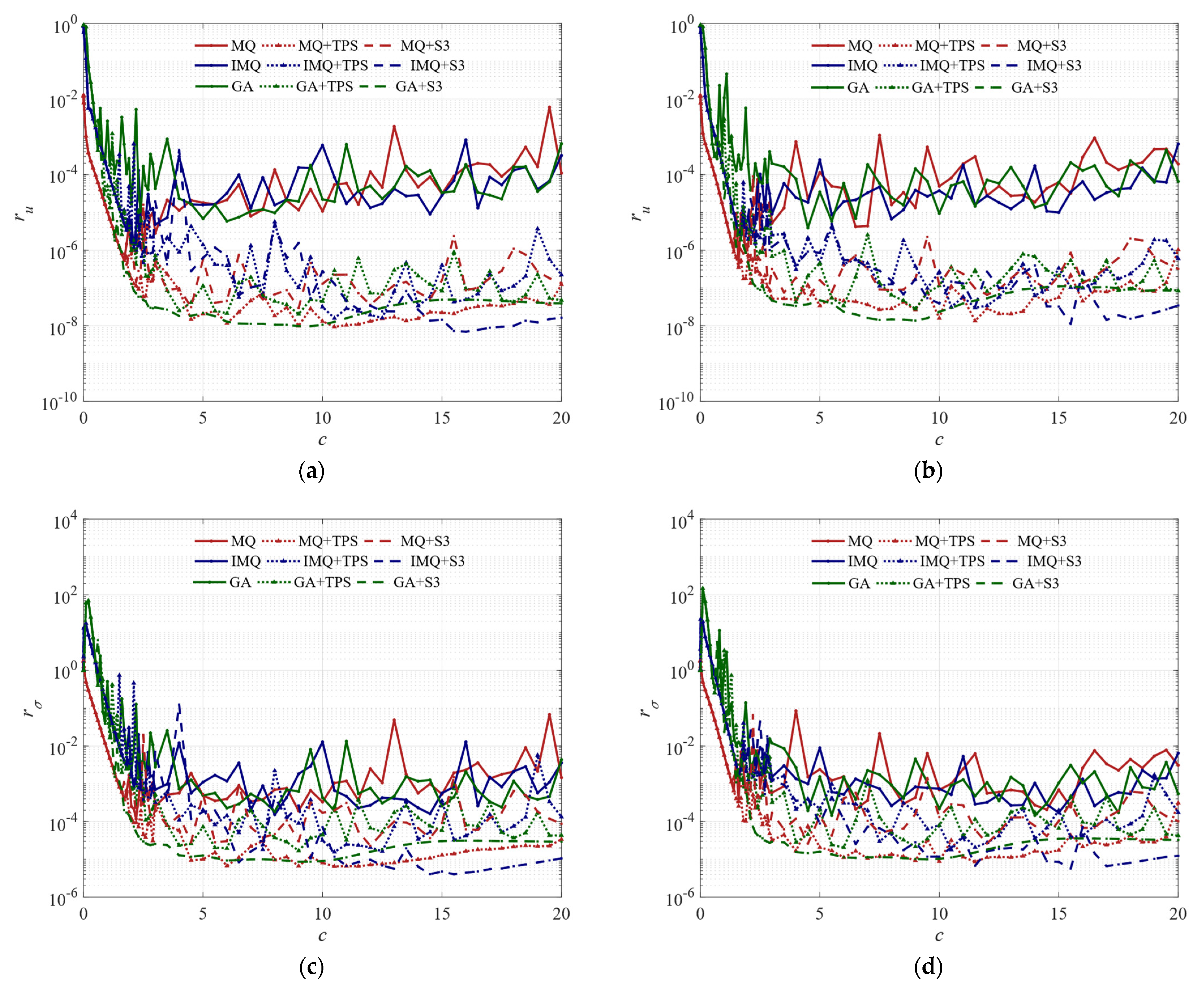
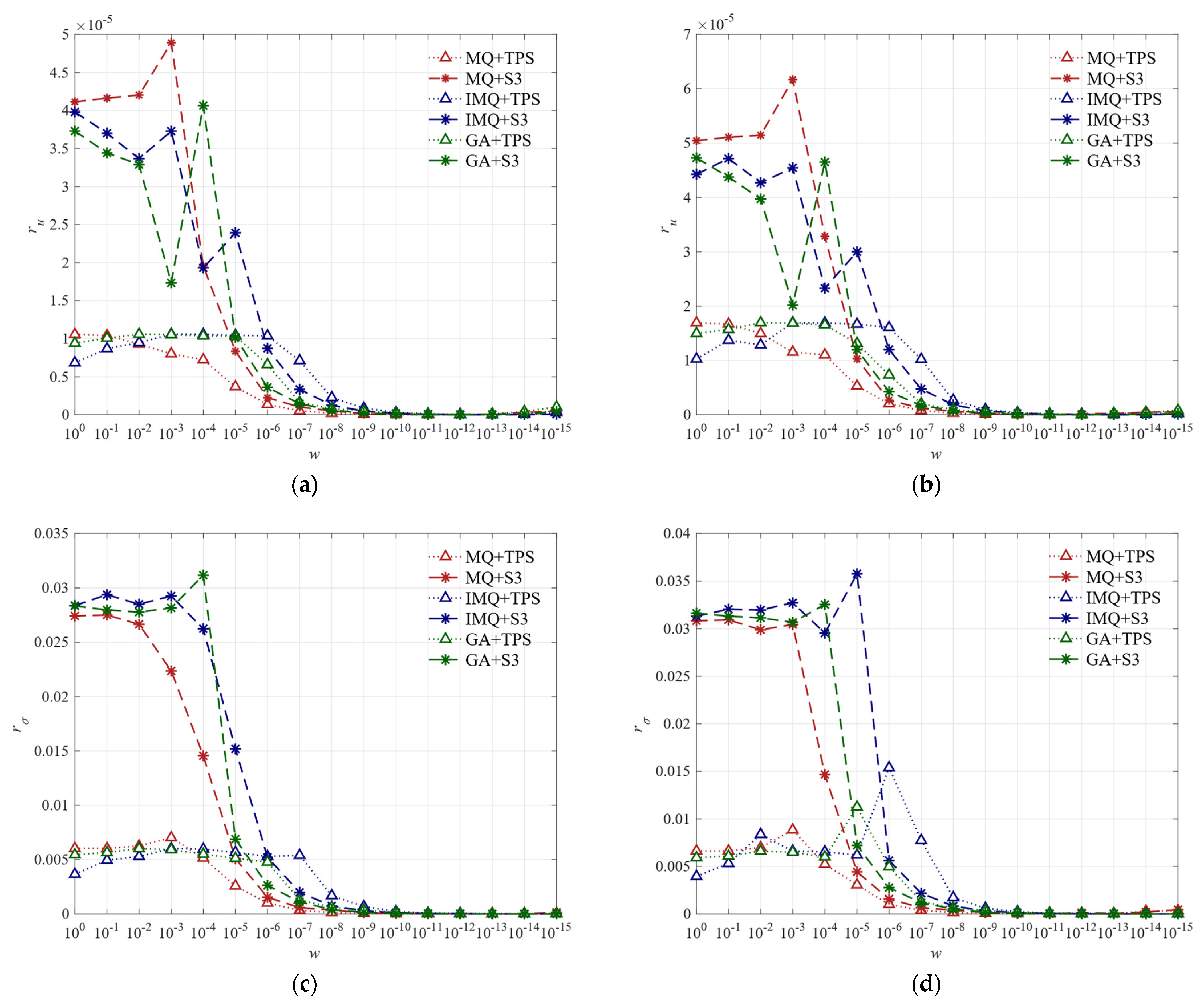
3.2.2. Effect of Parameters

When the meshless method analyzes nonlinear elastic problems, different radial basis function shape parameters impact the accuracy of the calculation. In addition to the shape parameter, the HRBF-CM includes a weight parameter w, so this section goes into detail. The influence of the shape parameter c and the weight parameter $w$ on the calculation results is studied. The relationships between $r_u, r_{\sigma }$ and the shape parameter c for the regular 73 × 13 (949 in total) nodes and the irregular 949 nodes are plotted in Figure 5. In particular, Figure 5a,b plot the relationship between the shape parameter c (varying from 10⁻⁴∼20) and the relative error of displacement $r_u$ and Figure 5c,d plot the corresponding relative error of $r_{\sigma }$. To explore the variation of other nodes, Figure 6 plots r_u and $r_{\sigma }$ relative to the weight parameter w for the regular 49 × 9 (441 in total) nodes and the irregular 441 nodes, where Figure 6a,b plot the relationship between the weight parameter w ([10⁰, 10⁻¹, 10⁻², …, 10⁻¹⁵]) and the relative error of displacement r_u, and Figure 6c,d plot the corresponding relative error of $r_{\sigma }$.

We can first see from these figures that the HRBF-CM has high accuracy. Figure 5 shows that the shape parameter c has a particular influence on the calculation progress of the conventional and hybrid radial basis functions. However, when the shape parameter takes an enormous value, the relative error of the hybrid radial basis function accuracy is still excellent. The trend shows that as the shape parameter increases, the relative error is smaller and more accurate. The hybrid radial basis function also contains a weighting parameter w. This article examines the effect of the weight parameter on accuracy in detail. We select 16 weighting parameters, and Figure 6 shows that the accuracy of all hybrid radial basis functions becomes higher as the weighting parameters are reduced, showing a convergence trend. The parameters for the TPS hybrid radial basis functions are smoother and not as volatile as those for the S3 hybrid radial basis functions. Table 4 and Table 5 give the optimal parameters for the regular and irregular nodes, and the optimal parameters are chosen by minimizing the relative error in the displacement r_u. These numerical results show that the HRBF-CM has better accuracy and better stability than the traditional RBF method when solving cantilever beam problems.

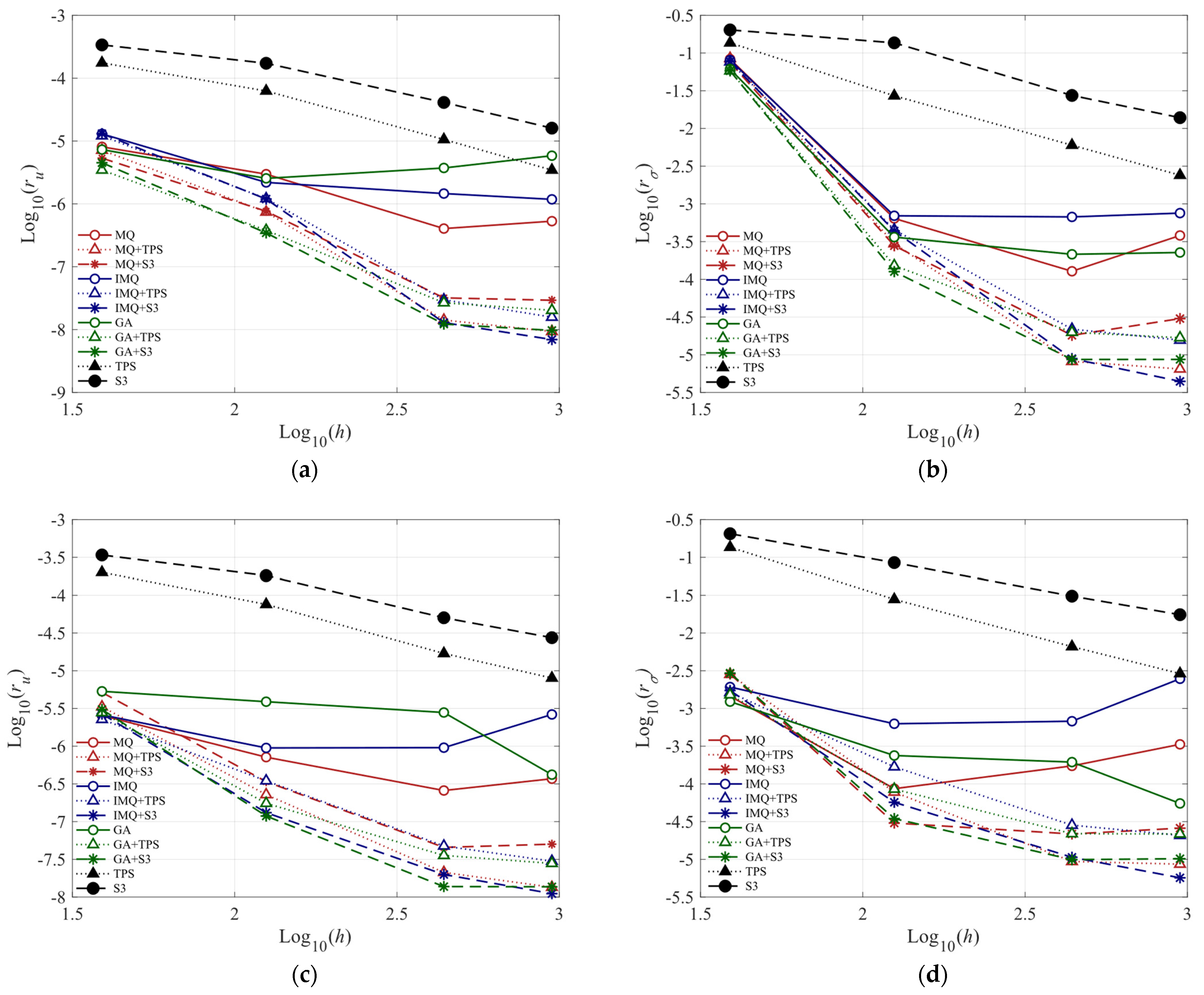
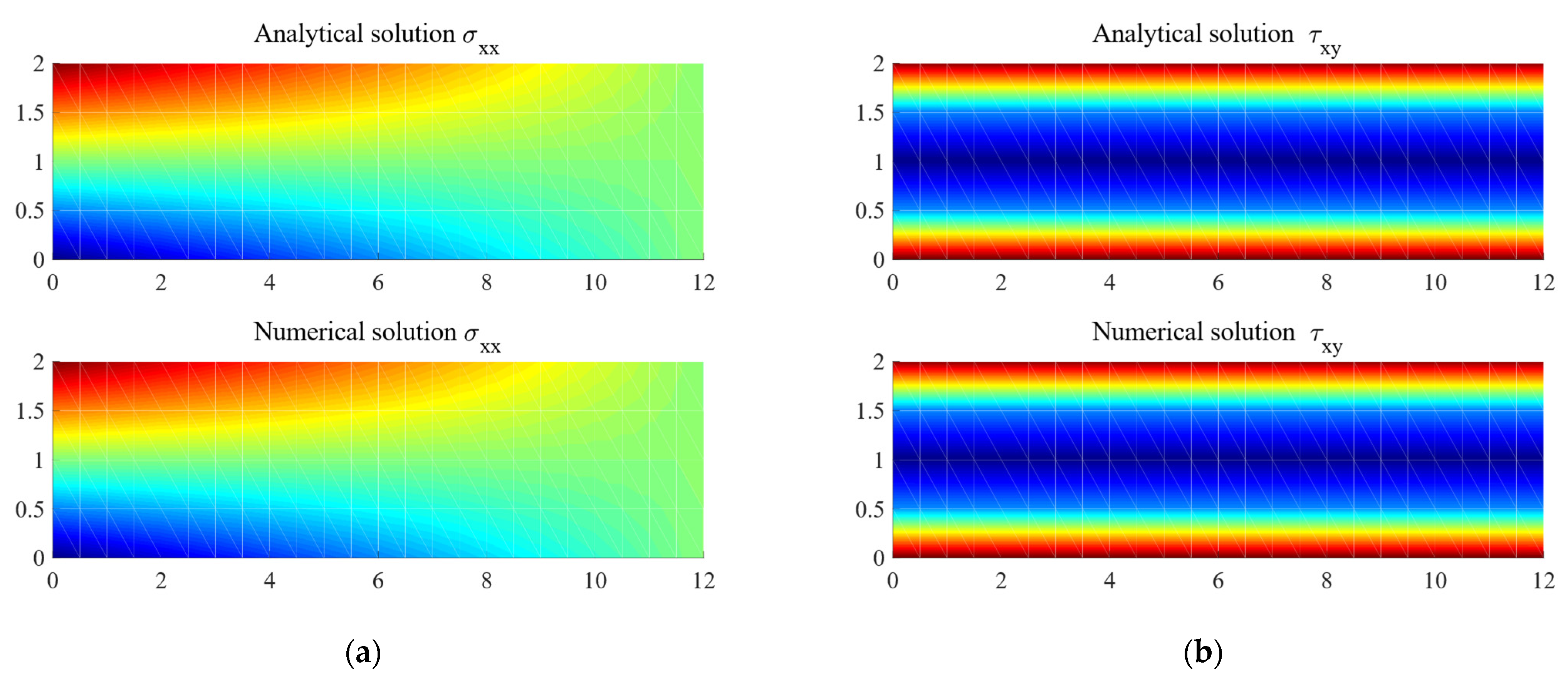
3.2.3. Convergence Analysis and Simulation

In this subsection, we analyze the convergence of the HRBF-CM using the cantilever beam as an example, and also give simulated plots of the computational results. In Table 4 and Table 5, we give the minimum relative error r_u and $r_{\sigma }$ for regular and irregular nodes, respectively, using different calculation methods. We draw the curves of the convergence diagram, as shown in Figure 7. Figure 7a,b show the convergence curves for stresses and displacements with regular node distribution. Figure 7c,d show the same items under irregular nodal distribution. h is the maximum size of the nodal arrangement.

The calculation results in Table 4 and Table 5 show that the HRBF-CM has excellent convergence properties. TPS and S3 converge slowly, and MQ, IMQ, and GA do not show good convergence. The relative errors r_u and $r_{\sigma }$ do not decrease as the number of nodes increases. For the small number of nodes, the accuracy of the traditional infinitely smooth RBF method is similar to the HRBF-CM. However, in the case of a large number of nodes, the HRBF-CM is more advantageous.

We plot the analytical and numerical solutions of the HRBF-CM (MQ + TPS) in the case of 73 × 13 regular nodes, as shown in Figure 8. Figure 8a represents the normal stress ${\sigma }_{xx}$ and Figure 8b shows the shear stress ${\tau }_{xy}$. It can be seen that the numerical solution and the analytical solution are highly consistent, and the calculation accuracy is very high.

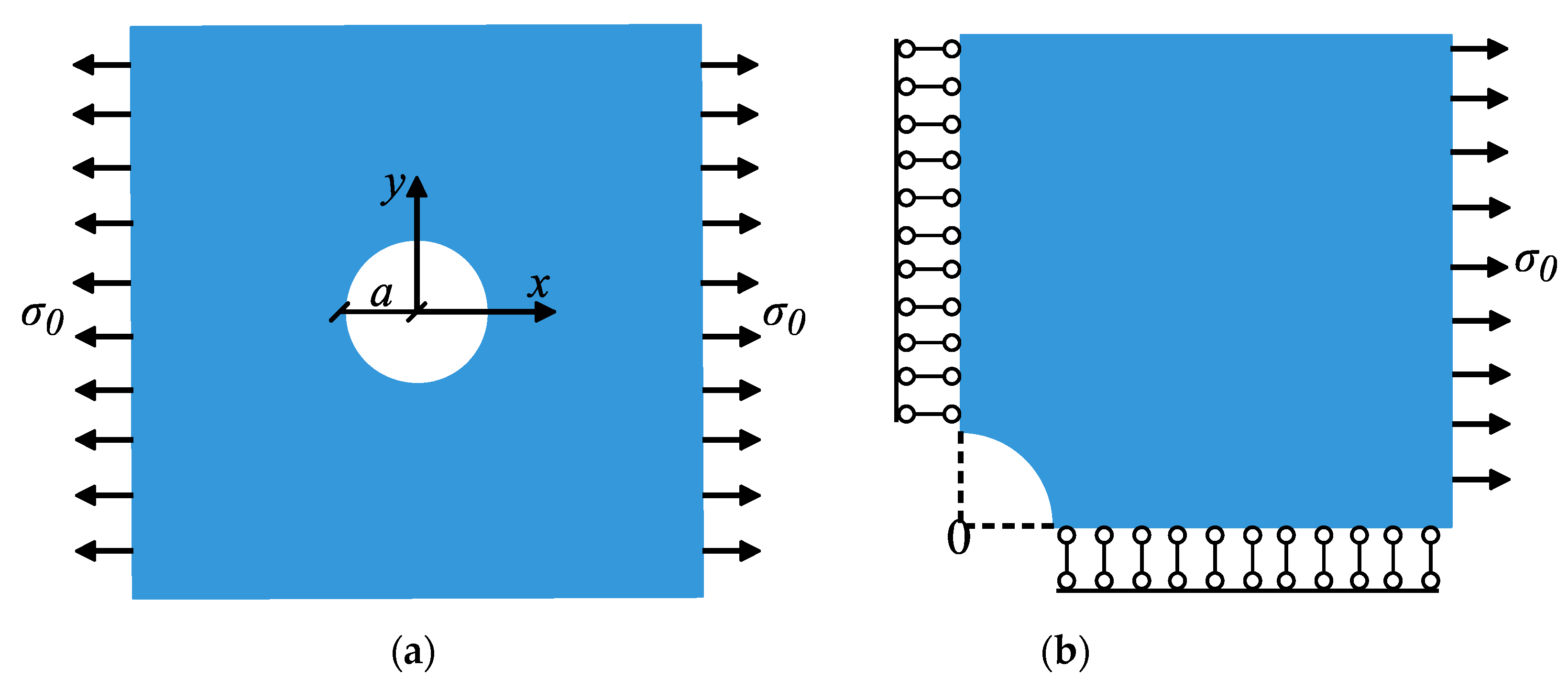
3.3. Plate with a Hole

For the third test problem, we consider a center circular hole plate with uniform tensile load ${\sigma }_0$ at infinity in the $x$ direction, as shown in Figure 9a. In actual computations, the geometric parameters and the material parameters are as follows: ${\sigma }_0=1$, L_x = 5, L_y = 5, a = 1, E = 1000, and μ = 0.3. Due to its symmetry, only a quarter of the model is considered in the calculation, as shown in Figure 9b.

We discuss the third numerical problem in Cartesian coordinates. This problem can also be discussed in polar coordinates [34]. Here, we only consider the Cartesian coordinate system. The analytical solution for displacement and stresses is as follows:

$$\{\begin{array}{l}{u}_x^{anal}=\frac{{\sigma }_{0}a}{8G}[\frac{x}{a}\left(\kappa +1\right)+2a\left(1+\kappa \right)\frac{x}{x^2+y^2}+2a\frac{x^3-3x{y}^2}{{\left(x^2+y^2\right)}^2}\left(1-\frac{a^2}{x^2+y^2}\right)],\hfill \\ u_y^{anal}=\frac{{\sigma }_{0}a}{8G}\left[\frac{y}{a}\left(\kappa -3\right)+2a\left(1-\kappa \right)\frac{y}{x^2+y^2}+2a\frac{3y{x}^2-y^3}{{\left(x^2+y^2\right)}^2}\left(1-\frac{a^2}{x^2+y^2}\right)\right],\hfill \end{array}$$

(24)

$$\{\begin{array}{l}{\sigma }_{xx}^{anal}={\sigma }_0\left[1-\frac{3}{2}\frac{a^2\left(x^2-y^2\right)}{{\left(x^2+y^2\right)}^2}-\frac{a^2}{{\left(x^2+y^2\right)}^3}\left(x^4+y^4-6x^2{y}^2\right)\left(1-\frac{3}{2}\frac{a^2}{x^2+y^2}\right)\right],\hfill \\ {\sigma }_{yy}^{anla}={\sigma }_0\left[-\frac{1}{2}\frac{a^2\left(x^2-y^2\right)}{{\left(x^2+y^2\right)}^2}+\frac{a^2}{{\left(x^2+y^2\right)}^3}\left(x^4+y^4-6x^2{y}^2\right)\left(1-\frac{3}{2}\frac{a^2}{x^2+y^2}\right)\right],\hfill \\ {\tau }_{xy}^{anal}=-{\sigma }_0\left[\frac{a^{2}xy}{{\left(x^2+y^2\right)}^2}+4a^{2}xy\frac{x^2-y^2}{{\left(x^2+y^2\right)}^3}\left(1-\frac{3}{2}\frac{a^2}{x^2+y^2}\right)\right].\hfill \end{array}$$

(25)

where $G=\frac{E}{2\left(1+\mu \right)}$ is the shear modulus. $\kappa =\frac{3-\mu }{1+\mu }.$ is the Kolosov constant.

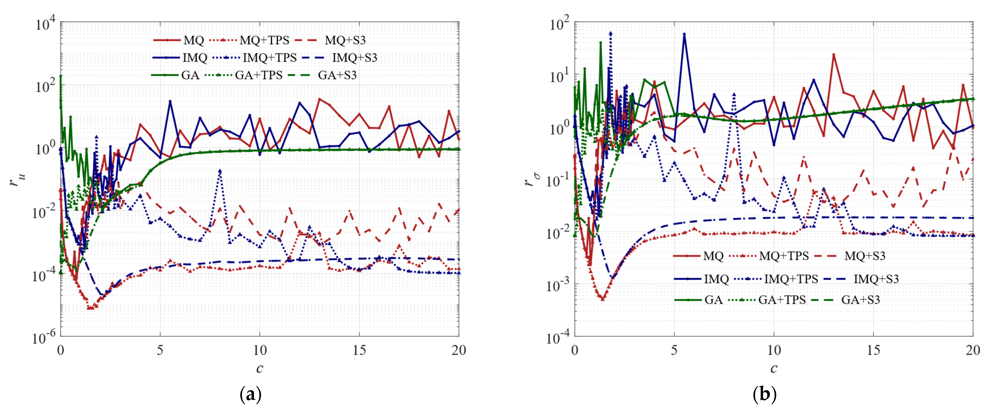
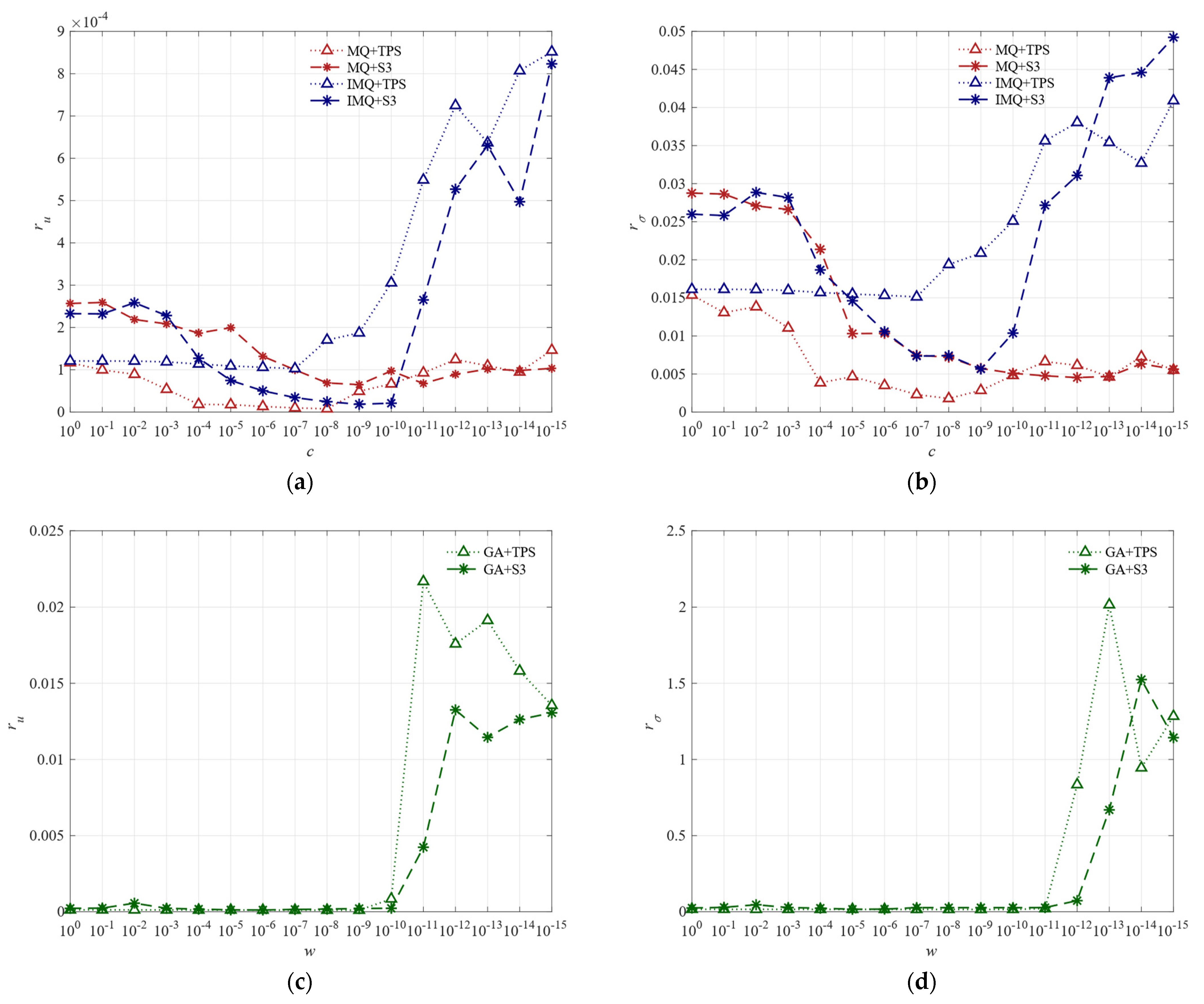
3.3.1. Effect of Parameters

We calculate three-node distributions for the plate with a hole, including 289, 626, and 1089. We plot the relationship between the shape parameter c and the relative errors r_u and $r_{\sigma }$ for the 1089 node distribution, respectively, in Figure 10. Figure 11 plots the relationship between the weight parameter w and the relative errors r_u and $r_{\sigma }$ for the same-sized nodes. Due to the difference in the order of magnitude of the errors, the relative error variations for MQ + TPS, MQ + S3, IMQ + TPS, and IMQ + S3 are plotted in Figure 11a,b to provide a more intuitive view. The relative error variations for GA + TPS and GA + S3 are plotted in Figure 11c,d.

As can be seen in Figure 10, the traditional RBF is not as accurate as HRBF when the shape parameter gradually increases. The GA radial basis function is not as accurate, and its variants GA + TPS, as well as GA + S3, are not advantageous either. As seen in Figure 11a,b, the relative error is more affected by the variation of the weighting parameter w, with better results for weighting parameters between [10⁻⁵, 10⁻⁶, 10⁻⁷, 10⁻⁸, 10⁻⁹]. The GA is less accurate, as seen in Figure 11c,d.

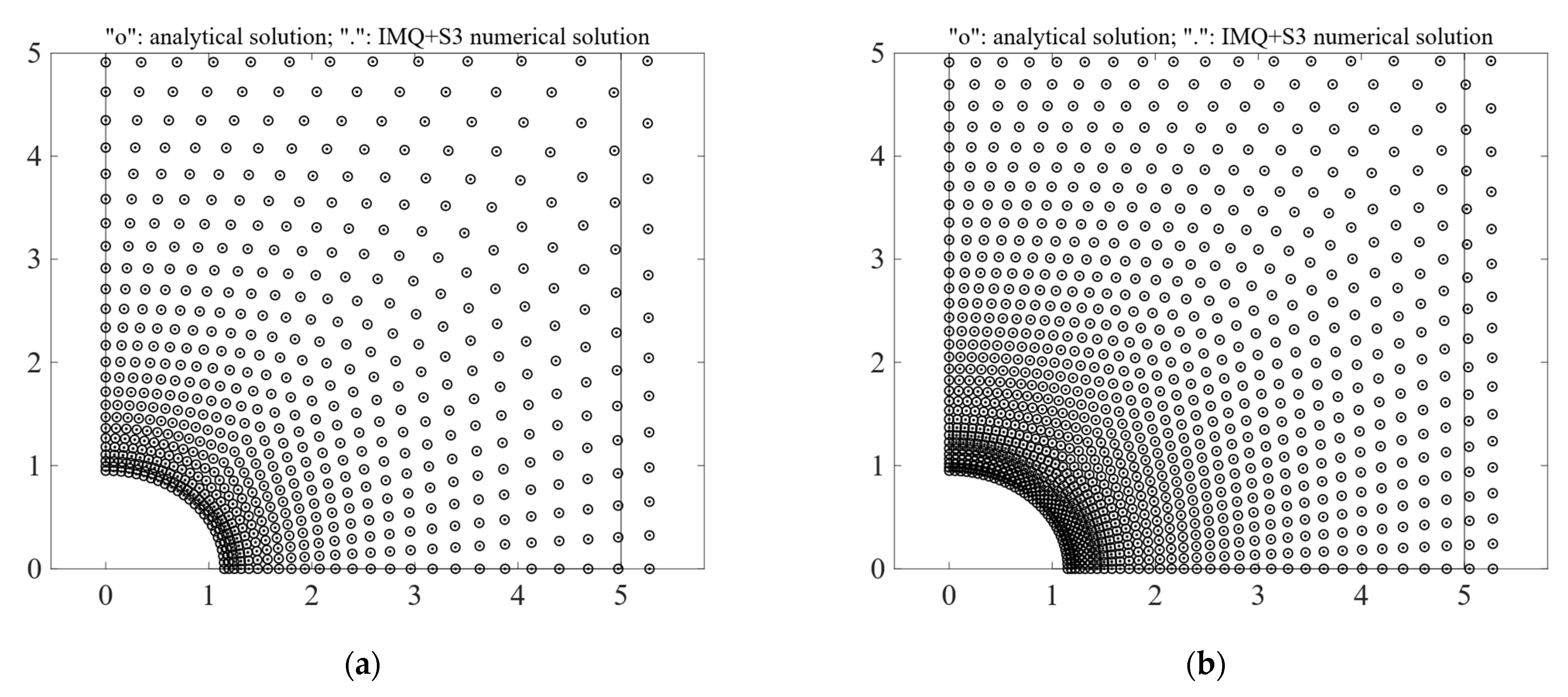
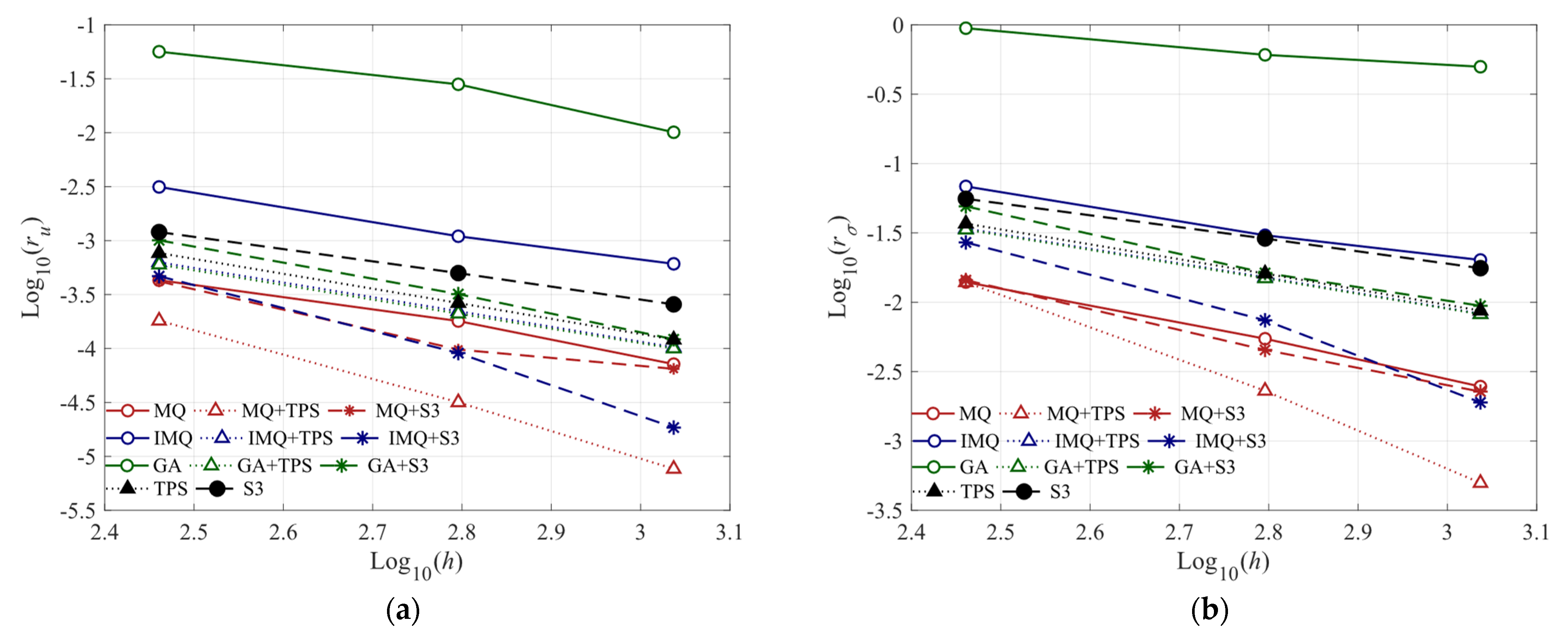
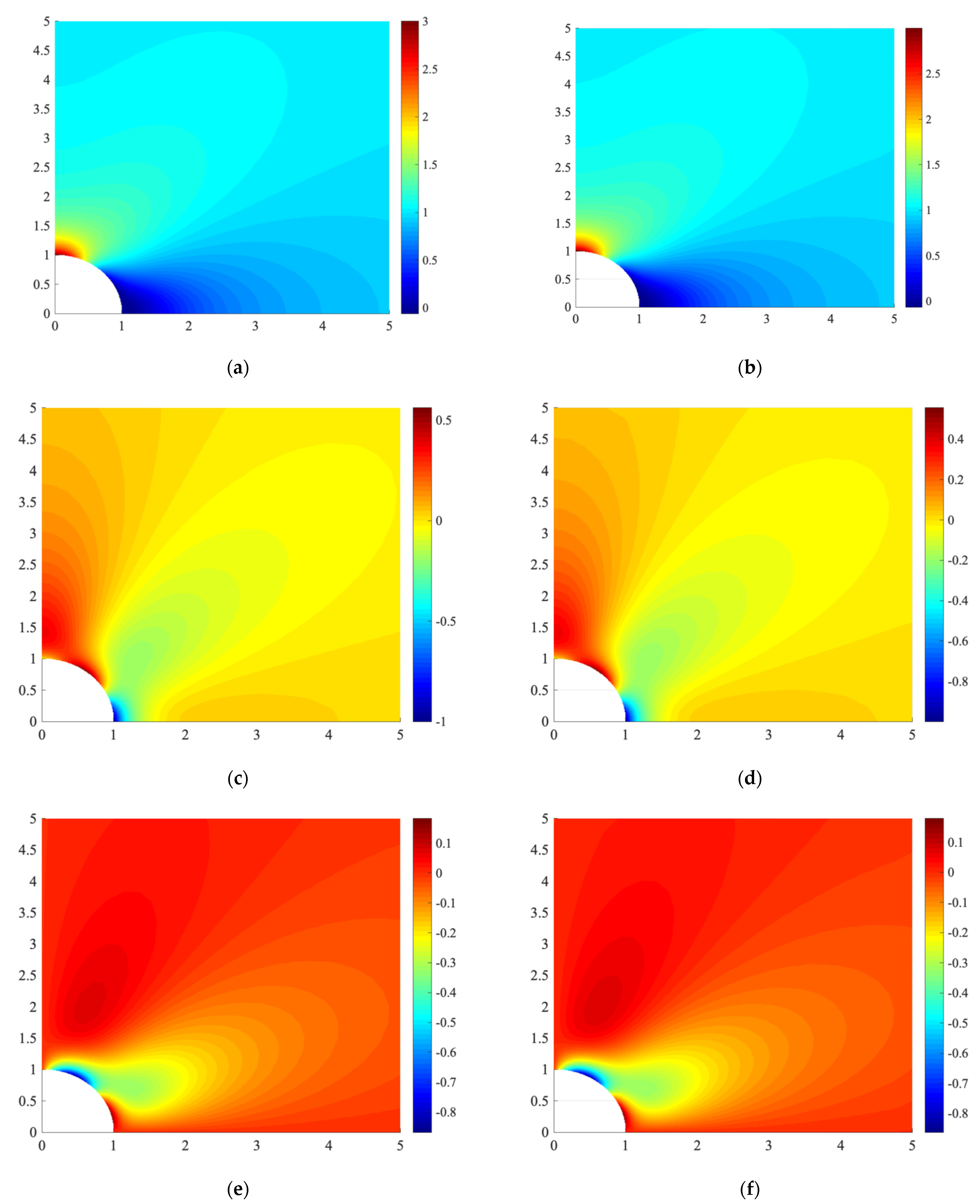
3.3.2. Convergence Analysis and Simulation

We investigate the convergence of the HRBF-CM in solving the plate with a hole by considering three-node distributions, namely 289, 626, and 1089. Figure 12 plots the results of the displacement calculations for nodes 625 and 1089. It can be seen that the settlement accuracy is very high. The calculation results for the other nodes are shown in

Table 6. Example 3: computational results of different methods.

Method		N = 289	N = 625	N = 1089
MQ	copt	0.9	0.8	0.8
	ru	4.2960 × 10−4	1.7965 × 10−4	7.1667 × 10−5
	$r_{\sigma }$	1.3975 × 10−2	5.4578 × 10−3	2.4684 × 10−3
	CPU (s)	0.1746	0.3531	1.1068
IMQ	copt	1.3	1.2	1.2
	ru	3.1431 × 10−3	1.0973 × 10−3	6.0918 × 10−4
	$r_{\sigma }$	6.8418 × 10−2	3.0396 × 10−2	2.0173 × 10−2
	CPU (s)	0.1658	0.2070	1.3669
GA	copt	1.8	2	2.1
	ru	5.6372 × 10−2	2.8088 × 10−2	1.0097 × 10−2
	$r_{\sigma }$	9.4539 × 10−1	6.0751 × 10−1	4.9868 × 10−1
	CPU (s)	0.0599	0.1048	0.5760
MQ + TPS	copt	(1.7,10−5)	(1.6,10−7)	(1.4,10−8)
	ru	1.8100 × 10−4	3.1703 × 10−5	7.6593 × 10−6
	$r_{\sigma }$	1.3936 × 10−2	2.2995 × 10−3	4.9781 × 10−4
	CPU (s)	0.1535	0.4709	1.5308
IMQ + TPS	copt	(20,10−7)	(20,10−7)	(20,10−7)
	ru	6.2954 × 10−4	2.2173 × 10−4	1.0269 × 10−4
	$r_{\sigma }$	3.4004 × 10−2	1.5125 × 10−2	8.2553 × 10−3
	CPU (s)	0.1371	0.5829	1.8389
GA + TPS	copt	(0.01,10−9)	(0.01,10−9)	(0.01,10−7)
	ru	5.9965 × 10−4	2.1045 × 10−4	9.9975 × 10−5
	$r_{\sigma }$	3.3397 × 10−2	1.4878 × 10−2	8.1967 × 10−3
	CPU (s)	0.0975	0.4265	1.3619
MQ + S3	copt	(0.9,10−8)	(0.9,10−12)	(0.8,10−9)
	ru	4.1938 × 10−4	9.7755 × 10−5	6.4772 × 10−5
	$r_{\sigma }$	1.4432 × 10−2	4.5325 × 10−3	2.2693 × 10−3
	CPU (s)	0.1264	0.4127	1.2019
IMQ + S3	copt	(2.5,10−6)	(2.5,10−8)	(2.2,10−9)
	ru	4.6816 × 10−4	9.0696 × 10−5	1.8502 × 10−5
	$r_{\sigma }$	2.6994 × 10−2	7.4137 × 10−3	1.8960 × 10−3
	CPU (s)	0.1495	0.5371	1.6242
GA+S3	copt	(0.4,10−5)	(0.8,10−5)	(0.8,10−5)
	ru	1.0062 × 10−3	3.1934 × 10−4	1.2175 × 10−4
	$r_{\sigma }$	4.9156 × 10−2	1.6263 × 10−2	9.4336 × 10−3
	CPU (s)	0.1173	0.3705	1.1097
TPS	ru	7.6646 × 10−4	2.6404 × 10−4	1.2074 × 10−4
	$r_{\sigma }$	3.6900 × 10−2	1.6100 × 10−2	8.7000 × 10−3
	CPU (s)	0.1215	0.2706	0.7952
S3	ru	1.2000 × 10−3	4.9997 × 10−4	2.5632 × 10−4
	$r_{\sigma }$	5.5700 × 10−2	2.8800 × 10−2	1.7600 × 10−2
	CPU (s)	0.1209	0.2032	0.5977

Note: The bold numbers represent the best calculated data.

. The optimal parameters listed in Table 6 are obtained by minimising the relative error r_u of the displacements. The calculation results show that the relative errors r_u and $r_{\sigma }$ decrease as the nodes increase. Figure 13 effectively shows the convergence characteristics, plotting the convergence curves for the nine kinds of radial basis functions. From these results, we find that the deformation HRBFs for all types of conventional radial basis functions are more accurate than the traditional radial basis functions, i.e., MQ + TPS and MQ + S3 are better than the MQ method, IMQ + TPS and IMQ + S3 are better than the MQ method, and GA + TPS and GA + S3 are more accurate than GA. When the number of nodes is 1089, IMQ + S3 has a displacement accuracy of up to 10⁻⁵ and a stress accuracy of 10⁻³. The HRBF-CM also has the highest accuracy for the other node distributions.

Figure 14a,b plot the analytical solution and the HRBF (IMQ + S3) solution for stress ${\sigma }_{xx}$. Figure 14c,d plot the analytical solution and the HRBF (IMQ + S3) solution for the stress ${\sigma }_{yy}$. Figure 14e,f plot the analytical and HRBF (IMQ + S3) solutions for the shear stress ${\tau }_{xy}$. These figures also show the excellent agreement between the analytical and numerical results.

It should be pointed out that the present study only considers the global collocation method to solve small-scale problems. We can use the local collocation method to solve large-scale problems in the future. The numerical examples are mainly focused on plane elastostatic symmetry problems. However, it can be extended to three-dimensional elastostatic problems to verify the effectiveness of the HRBF-CM.

4. Conclusions

The traditional RBF methods are widely used in many areas of scientific computing, such as interpolating multi-dimensional scattered data and solving PDEs. The HRBF is constructed based on infinite smooth RBFs and piecewise smooth RBFs. It does inherit the advantages of both RBFs, making HRBFs both spectrally convergent and stable. Inspired by Manzoor, [24] used the HRBF to solve the Burgers’ equation; we study his HRBF in detail in this paper, using three elastostatic symmetric problems. The sensitivity analysis of the HBRF concerning the number of nodes N, the weight parameter w, and the shape parameter c is analyzed. The ability of the HRBF-CM to fit the data under different shape parameters and weight parameters is investigated. The numerical results of the HRBF are compared with those of the analytical solutions and other numerical methods, and excellent agreements can be found.

References

1. Hardy, R.L. Multiquadric equations of topography and other irregular surfaces. J. Geophys. Res. 1971, 76, 1905–1915. [Google Scholar] [CrossRef]
2. Buhmann, M.D. Radial basis functions. Acta Numer. 2000, 9, 1–38. [Google Scholar] [CrossRef] [Green Version]
3. Kansa, E.J. Multiquadrics—A scattered data approximation scheme with applications to computational fluiddynamics—II solutions to parabolic, hyperbolic and elliptic partial differential equations. Comput. Math. Appl. 1990, 19, 147–161. [Google Scholar] [CrossRef] [Green Version]
4. Lee, M.B.; Lee, Y.L.; Sunwoo, Y.L.; Yoon, J. Some issues on interpolation matrices of locally scaled radial basis functions. Appl. Math. Comput. 2011, 217, 5011–5014. [Google Scholar] [CrossRef]
5. Fasshauer, G.E.; Zhang, J.G. On choosing “optimal” shape parameters for RBF approximation. Numer. Algorithms 2007, 45, 345–368. [Google Scholar] [CrossRef]
6. Franke, C.; Schaback, R. Solving partial differential equations by collocation using radial basis functions. Appl. Math. Comput. 1998, 93, 73–82. [Google Scholar] [CrossRef]
7. Hardy, R.L. A contribution of the multiquadric method: Interpolation of potential inside the earth. Comput. Math. Appl. 1992, 24, 81–97. [Google Scholar] [CrossRef] [Green Version]
8. Rippa, S. An algorithm for selecting a good value for the parameter c in radial basis function interpolation. Adv. Comput. Math. 1999, 11, 193–210. [Google Scholar] [CrossRef]
9. Diederichs, B.; Iske, A. Improved estimates for condition numbers of radial basis function interpolation matrices. J. Approx. Theory 2019, 238, 38–51. [Google Scholar] [CrossRef]
10. Majdisova, Z.; Skala, V. Radial basis function approximations: Comparison and applications. Appl. Math. Model. 2017, 51, 728–743. [Google Scholar] [CrossRef] [Green Version]
11. Kansa, E.J.; Carlson, R. Improved accuracy of multi-quadric interpolation using variable shape parameters. Comput. Math. Appl. 1992, 24, 20–99. [Google Scholar] [CrossRef] [Green Version]
12. Scotta, A.S.; Derek, S. A random variable shape parameter strategy for radial basis function approximation methods. Eng. Anal. Bound. Elem. 2009, 33, 1239–1245. [Google Scholar]
13. Biazar, J.; Hosami, M. An interval for the shape parameter in radial basis function approximation. Appl. Math. Comput. 2017, 315, 131–149. [Google Scholar] [CrossRef]
14. Ahmad, G.; Ehsan, M.; Hamed, R. On the new variable shape parameter strategies for radial basis function. Comput. Appl. Math. 2015, 34, 691–704. [Google Scholar]
15. Stolbunov, V.; Nair, P.B. Sparse radial basis function approximation with spatially variable shape parameters. Appl. Math. Comput. 2018, 330, 170–184. [Google Scholar] [CrossRef]
16. Bayona, V.; Moscoso, M.; Kindelan, M. Optimal variable shape parameter for multiquadric based RBF-FD method. J. Comput. Phys. 2012, 231, 2466–2481. [Google Scholar] [CrossRef]
17. Zhang, Y.M. An accurate and stable RBF method for solving partial differential equations. Appl. Math. Lett. 2019, 97, 93–98. [Google Scholar] [CrossRef]
18. Nadir, B.; Mohammed, O.; Minh-Tuan, N.; Abderrezak, S. Optimal trajectory generation method to find a smooth robot joint trajectory based on multiquadric radial basis functions. Int. J. Adv. Manuf. Technol. 2022, 120, 297–312. [Google Scholar] [CrossRef]
19. Feng, L.T.; Katupitiya, J. Radial basis function-based vector field algorithm for wildfire boundary tracking with UAVs. Comput. Appl. Math. 2022, 41, 124. [Google Scholar] [CrossRef]
20. Swetha, K.; Eldho, T.I.; Singh, L.G.; Kumar, A.V. Groundwater flow simulation in a confined aquifer using local radial point interpolation meshless method (LRPIM). Eng. Anal. Bound. Elem. 2022, 134, 637–649. [Google Scholar] [CrossRef]
21. Parand, K.; Hemami, M. Numerical study of astrophysics equations by meshless collocation method based on compactly supported radial basis function. Int. J. APPL. Comput. Math. 2017, 3, 1053–1075. [Google Scholar] [CrossRef] [Green Version]
22. Karimi, N.; Kazem, S.; Ahmadian, D.; Adibi, H.; Ballestra, L.V. On a generalized Gaussian radial basis function: Analysis and applications. Eng. Anal. Bound. Elem. 2020, 112, 46–57. [Google Scholar] [CrossRef]
23. Chen, Y.T.; Cao, Y. A coupled RBF method for the solution of elastostatic problems. Math. Probl. Eng. 2021, 2121, 6623273. [Google Scholar] [CrossRef]
24. Hussain, M. Hybrid radial basis function methods of lines for the numerical solution of viscous Burgers’ equation. J. Comput. Appl. Math. 2021, 40, 107. [Google Scholar] [CrossRef]
25. Zhang, X.; Song, K.Z.; Lu, M.W.; Liu, X. Meshless methods based on collocation with radial basis functions. Comput. Mech. 2000, 26, 333–343. [Google Scholar] [CrossRef]
26. Wendland, H. Piecewise polynomial positive definite and compactly supported radial basis functions of minimal degree. Adv. Comput. Math. 1995, 4, 389–396. [Google Scholar] [CrossRef]
27. Tolstykh, A.I.; Shirobokov, D.A. On using radial basis functions in a “finite difference mode” with applications to elasticity problems. Comput. Mech. 2003, 33, 68–79. [Google Scholar] [CrossRef]
28. Liu, G.R.; Gu, Y.T. A local radial point interpolation method (LRPIM) for free vibration analyses of 2-D solids. J. Sound Vib. 2001, 246, 29–46. [Google Scholar] [CrossRef] [Green Version]
29. Wang, J.G.; Liu, G.R. A point interpolation meshless method based on radial basis functions. Int. J. Numer. Methods Eng. 2002, 54, 1623–1648. [Google Scholar] [CrossRef]
30. Wang, J.G.; Liu, G.R. On the optimal shape parameters of radial basis functions used for 2-D meshless methods. Comput. Methods Appl. Mech. Eng. 2002, 191, 2611–2630. [Google Scholar] [CrossRef]
31. Cao, Y.; Yao, L.Q.; Yi, S.C. A weighted nodal-radial point interpolation meshless method for 2D solid problems. Eng. Anal. Bound. Elem. 2014, 39, 88–100. [Google Scholar] [CrossRef]
32. Simonenko, S.; Bayona, V.; Kindelan, M. Optimal shape parameter for the solution of elastostatic problems with the RBF method. J. Eng. Math. 2014, 85, 115–129. [Google Scholar] [CrossRef]
33. Mishra, P.K.; Nath, S.K.; Kosec, G.; Sen, M.K. An improved radial basis-pseudospectral scheme with hybrid Gaussian-cubic kernels. Eng. Anal. Bound. Elem. 2017, 80, 162–171. [Google Scholar] [CrossRef] [Green Version]
34. Liu, Z.; Gao, H.F.; Wei, G.F.; Wang, Z.M. The meshfree analysis of elasticity problem utilizing radial basis reproducing kernel particle method. Results Phys. 2020, 17, 103037. [Google Scholar] [CrossRef]
35. Chen, Z.Y.; Zhao, Q.F.; Lim, C.W. A new static-dynamic equivalence beam bending approach for the stability of a vibrating beam. Mech. Adv. Mater. Struct. 2021, 28, 999–1009. [Google Scholar] [CrossRef]
Figure 1. Example 1: a patch with 13 nodes.
Symmetry 14 01476 g001
Figure 2. Example 2: cantilever beam.
Symmetry 14 01476 g002
Figure 3. Example 2: (a) 441 regular node distribution; (b): 441 irregular node distribution.
Symmetry 14 01476 g003
Figure 4. Example 2: displacement computational results using HRBF (GA + S3)−(a): 441 regular nodes distribution; (b): 441 irregular node distribution.
Symmetry 14 01476 g004
Figure 5. Example 2: relationship between relative errors ru and r σ and shape parameter c—(a,c): 949 regular node distribution; (b,d): 949 irregular node distribution.
Symmetry 14 01476 g005
Figure 6. Example 2: relationship between relative errors and weight parameter—(a,c): 441 regular nodes; (b,d): 441 irregular nodes.
Symmetry 14 01476 g006
Figure 7. Example 2: convergence study−(a): regular node distribution, convergence curves of ru; (b): regular node distribution, convergence curves of r σ ; (c): irregular node distribution, convergence curves of ru; (d): irregular node distribution, convergence curves of r σ .
Symmetry 14 01476 g007
Figure 8. Example 2: stress computational results using HRBF (MQ + TPS, regular 949 nodes). (a) Normal stress σ x x ; (b): shear stress τ x y .
Symmetry 14 01476 g008
Figure 9. Example 3: (a): plate with a hole; (b): a quarter of the model.
Symmetry 14 01476 g009
Figure 10. Example 3: 1089 node distribution−(a): relationship between relative errors ru and shape parameter c; (b): relationship between relative errors r σ and shape parameter c.
Symmetry 14 01476 g010
Figure 11. Example 3: 1089 node distribution—(a,c): relationship between relative errors ru and shape parameter w; (b,d): relationship between relative errors r σ and shape parameter w.
Symmetry 14 01476 g011
Figure 12. Example 3: displacement computational results using the HRBF (IMQ + S3)—(a): 625 nodes; (b): 1089 nodes.
Symmetry 14 01476 g012
Figure 13. Example 3: convergence study—(a): convergence curves of ru; (b): convergence curves of r σ .
Symmetry 14 01476 g013
Figure 14. Example 3: stress computational results using HRBF (IMQ + S3, 1089 nodes)—(a): analytical solution of normal stress σ x x ; (b): numerical solution of normal stress σ x x ; (c): analytical solution of normal stress σ y y ; (d): numerical solution of normal stress σ y y ; (e): analytical solution of shear stress τ x y ; (f): numerical solution of shear stress τ x y .
Symmetry 14 01476 g014