Analysis of Fractional-Order System of One-Dimensional Keller–Segel Equations: A Modified Analytical Method

Abstract

In this paper, an analytical method is implemented to solve fractional-order Keller–Segel equations. The Yang transformation along with the Adomian decomposition method is implemented to obtain the solution of the given problems. The present method has an edge over other techniques as it does not need extra calculations and materials. The validity of the suggested technique is verified by considering some numerical problems. The results obtained confirm the better accuracy of the current technique. The suggested technique has a lesser number of calculations and is straightforward to apply and therefore can be applied to other fractional-order partial differential equations.

1. Introduction

Fractional calculus (FC) has emerged as a new mathematical tool for describing nonlocal structures. In recent generations, fractional derivatives have been used to mathematically explain a variety of physical challenges, and these interpretations have shown good results when used to mimic real-world circumstances. Hadamard, Riemann–Liouville, Coimbra, Grunwald–Letnikov, Riesz, Weyl, Liouville Caputo, Atangana–Baleanu, Caputo–Fabrizio and some others, provided essential definitions of fractional operators [1,2,3,4,5]. To analyse the nonlinear FPDE solutions, several sophisticated approaches for discovering precise solutions have been devised, such as the Hermite colocation method [6], the optimal homotopy asymptotic technique [7], the Adomian decomposition method [8], the homotopy perturbation transform method [9], the Pade approximation and homotopy-Pade technique [10], the invariant subspace method [11], the q-homotopy analysis transform method [12], the homotopy analysis Sumudu transform method [13] and the Sumudu transform series expansion method [14]. Without applying perturbation techniques, the homotopy analysis technique converts a problem into an infinite number of linear problems. To obtain a convergent series solution [15,16], this approach uses the idea of homotopy from topology. The Laplace homotopy perturbation technique is a hybrid of Liao’s [17] suggested homotopy analysis approach and the Laplace transform [18]. The study of partial differential equations, particularly those derived from finance mathematics, is where the elegance of symmetry analysis is most apparent. The secret of nature is symmetry, but the majority of natural observations lack symmetry. The occurrence of spontaneous symmetry breaking is a successful method for concealing symmetry. There are two types of symmetry: finite and infinitesimal. There can be continuous or discrete symmetries for finite symmetries. The natural symmetries of symmetry and time reversed are discrete, whereas space is a continuous transformation. Mathematicians have been fascinated by patterns for centuries. The nineteenth century witnessed the emergence of systematic classifications of planar and spatial patterns. Unfortunately, accurately solving nonlinear fractional differential equations has proven to be quite difficult [19].

Chemotaxis is the movement of cells that is guided by a chemical substance differential. It is crucial in developmental biology and, more broadly, in cell population self-organisation. Evelyn Keller and Lee Segel proposed the chemotaxis first mathematical model in 1970. They introduced parabolic methods for explaining the chemical-attraction-based cellular slime’s mould aggregation process [20]. In this study, we examine the fractional-order system of a Keller–Segel (KS) model of the form as

$$\begin{array}{cc}\hfill \frac{{\partial }^{\delta }}{\partial {\tau }^{\delta }}\mathcal{V}(\zeta ,\tau )& =\alpha \frac{{\partial }^2}{\partial {\zeta }^2}\mathcal{V}(\zeta ,\tau )-\frac{\partial }{\partial \zeta }\left(\mathcal{V}(\zeta ,\tau )\frac{\partial \chi \left(\phi \right)}{\partial \zeta }\right)\hfill \\ \hfill \frac{{\partial }^{\delta }}{\partial {\tau }^{\delta }}\phi (\zeta ,\tau )& =\beta \frac{{\partial }^2}{\partial {\zeta }^2}\phi (\zeta ,\tau )+\gamma \mathcal{V}(\zeta ,\tau )-\sigma \phi (\zeta ,\tau ),\hfill \end{array}$$

with initial conditions

$$\mathcal{V}(\zeta ,0)={\mathcal{V}}_0\left(\zeta \right),\phi (\zeta ,0)={\phi }_0\left(\zeta \right),\zeta \in I.$$

The unknown term $\mathcal{V}(\zeta ,\tau )$ denotes the amoebae of concentration and $\phi (\zeta ,\tau )$ expresses the chemical substance of concentration; $\frac{\partial }{\partial \zeta }\left(\mathcal{V}(\zeta ,\tau )\frac{\partial \chi \left(\phi \right)}{\partial \zeta }\right)$ denotes the chemotactic term and shows that the cells are sensitive to the chemicals and are attracted by them; $\chi \left(\phi \right)$ is the sensitivity function while $\alpha ,\beta ,\gamma$ and $\sigma$ are positive constants; $0<\delta \le 1$ is the parameter representing the order of the fractional derivative. The KS model has recently been widely studied. Atangana, for example, used a modified homotopy perturbation, the homotopy decomposition, and the Laplace transform approach to solve the KS model in [21,22,23]. In [24], Zayernouri created a fractional class of implicit Adams–Moulton and explicit Adams–Bashforth procedures. The fractional derivative of Liouville–Caputo was explored. The modified homotopy analysis transform technique (MHATM) is an analytical methodology that combines the homotopy analysis method and the Laplace transform with a homotopy polynomial and was proposed in [25]. The MHATM technique with homotopy polynomial was invented by the authors in [25] for solving time-fractional KS equations using the fractional derivative of Liouville–Caputo. The suggested method produced a convergence study of MHATM, which was validated using several graphical representations.

It is worth mentioning that Adomian first presented the Adomian decomposition method (ADM) in 1980. This is a useful methodology for solving systems of differential equations that emerge in physical problems, both numerically and explicitly, and it has proven to be a very reliable technique for both boundary- and initial-value problems. Here, in particular, papers [26,27,28,29,30,31,32,33] address the application of ADM to various fractional transport models, whilst paper [34] discusses some nonstandard definitions of fractional derivatives. Sources [35,36,37,38] contain developments and/or reviews of various numerical approaches to transport problems, while [39] proposes an interesting perturbational approach to construct analytical approximations. Finally, the review paper [40] contains a comprehensive number of modern applications of fractional calculus.

In this article, we combine the Adomian decomposition method and Yang’s transform method, called the Yang decomposition method (YDM). When compared to other numerical techniques, we can see that the YDM does not require any perturbation or liberalisation to determine the dynamical behaviour of complicated dynamical systems. The physical behaviour of the one-dimensional KS equation is investigated in this paper by using the YDM and the Yang transform to translate the problem into an algebraic type, and the nonlinear functions are decomposed with the help of Adomian polynomials [41,42,43].

2. Preliminary Concepts

We provide the fundamental definitions that will be used throughout the article. For the purpose of simplification, we write the exponential decay kernel as, $K(\tau ,\varrho )=e^{-\delta (\tau -\varrho )/(1-\delta )}$.

Definition 1.

The Caputo–Fabrizio derivative is given as follows [44]:

$${}^{CF}{D}_{\tau }^{\delta }\left[\mathbb{P}\left(\tau \right)\right]=\frac{N\left(\delta \right)}{1-\delta }{\int }_0^{\tau }{\mathbb{P}}^{{}^{\prime }}\left(\varrho \right)K(\tau ,\varrho )d\varrho ,0<\delta \le 1.$$

(1)

$N\left(\delta \right)$ is the normalisation function with $N\left(0\right)=N\left(1\right)=1$.

$${}^{CF}{D}_{\tau }^{\delta }\left[\mathbb{P}\left(\tau \right)\right]=\frac{N\left(\delta \right)}{1-\delta }{\int }_0^{\tau }[\mathbb{P}\left(\tau \right)-\mathbb{P}\left(\varrho \right)]K(\tau ,\varrho )d\varrho .$$

(2)

Definition 2.

The fractional integral Caputo–Fabrizio is given as [44]

$${}^{CF}{I}_{\tau }^{\delta }\left[\mathbb{P}\left(\tau \right)\right]=\frac{1-\delta }{N\left(\delta \right)}\mathbb{P}\left(\tau \right)+\frac{\delta }{N\left(\delta \right)}{\int }_0^{\tau }\mathbb{P}\left(\varrho \right)d\varrho ,\tau \ge 0,\delta \in (0,1].$$

(3)

Definition 3.

For $N\left(\delta \right)=1$, the following result shows the Caputo–Fabrizio derivative of the Laplace transform [44]:

$$L\left[{}^{CF}{D}_{\tau }^{\delta }\left[\mathbb{P}\left(\tau \right)\right]\right]=\frac{sL\left[\mathbb{P}\right(\tau \left)\right]-\mathbb{P}\left(0\right)}{s+\delta (1-s)}.$$

(4)

Definition 4.

The Yang transform of $\mathbb{P}\left(\tau \right)$ is expressed as [45]

$$\mathbb{Y}\left[\mathbb{P}\left(\tau \right)\right]=\chi \left(s\right)={\int }_0^{\infty }\mathbb{P}\left(\tau \right)e^{-\frac{\tau }{s}}d\tau .\tau >0,$$

(5)

Remark 1.

The Yang transform of a few useful functions is defined as follows:

$$\begin{array}{cc}\hfill \mathbb{Y}\left[1\right]=& s,\hfill \\ \hfill \mathbb{Y}\left[\tau \right]=& s^2,\hfill \\ \hfill \mathbb{Y}\left[{\tau }^i\right]=& \Gamma (i+1)s^{i+1}.\hfill \end{array}$$

(6)

Definition 5.

The inverse Yang transform ${\mathbb{Y}}^{-1}$ is defined by

$${\mathbb{Y}}^{-1}\left[\mathbb{P}\left(\tau \right)\right]=\frac{1}{2\pi \iota }{\int }_{\alpha -\iota \infty }^{\alpha +\iota \infty }h\left(\frac{1}{s}\right)e^{s\tau }sds=\Sigma residuesofh\left(\frac{1}{s}\right)e^{s\tau }s.$$

Lemma 1 (Laplace–Yang duality).

Let the Laplace transform of $\mathbb{P}\left(\tau \right)$ be $F\left(s\right)$, then $\chi \left(s\right)=F(1/s)$ [46].

Lemma 2.

Let $\mathbb{P}\left(\tau \right)$ be a continuous function, then the Yang transform of the Caputo–Fabrizio derivative of $\mathbb{P}\left(\tau \right)$ is defined by [46]

$$\mathbb{Y}\left[{}^{CF}{D}_{\tau }^{\delta }\left[\mathbb{P}\left(\tau \right)\right]\right]=\frac{\mathbb{Y}\left[\mathbb{P}\right(\tau \left)\right]-s\mathbb{P}\left(0\right)}{1+\delta (s-1)}.$$

(7)

3. Fundamental Concept of the Yang Decomposition Method

We consider the following nonhomogenous fractional-order nonlinear partial differential equation with initial condition:

$$\begin{array}{cc}\hfill \frac{{\partial }^{\delta }\mathcal{V}(\zeta ,\tau )}{\partial {\tau }^{\delta }}& =G\left(\mathcal{V}\right(\zeta ,\tau \left)\right)+N\left(\mathcal{V}\right(\zeta ,\tau \left)\right)+\ell (\zeta ,\tau ),0<\delta \le 1\hfill \\ \hfill \mathcal{V}(\zeta ,0)& =\varphi \left(\zeta \right),\hfill \end{array}$$

(8)

where G is a linear and N a nonlinear term. Using the Yang transform on (8), we get

$$\begin{array}{c}\hfill \mathbb{Y}\left[D_{\tau }^{\delta }\mathcal{V}(\zeta ,\tau )\right]=\mathbb{Y}\left[G\left(\mathcal{V}(\zeta ,\tau )\right)\right]+\mathbb{Y}\left[N\left(\mathcal{V}(\zeta ,\tau )\right)\right]+\mathbb{Y}[\ell (\zeta ,\tau )],\end{array}$$

(9)

$$\begin{array}{c}\hfill \frac{1}{(1+\delta (s-1\left)\right)}\mathbb{Y}\left[\mathcal{V}(\zeta ,\tau )\right]-s\mathcal{V}(\zeta ,0)=\mathbb{Y}\left[G\left(\mathcal{V}(\zeta ,\tau )\right)\right]+\mathbb{Y}\left[N\left(\mathcal{V}(\zeta ,\tau )\right)\right]+\mathbb{Y}[\ell (\zeta ,\tau )].\end{array}$$

(10)

Using the initial condition in Equation (10), we achieve:

$$\begin{array}{c}\hfill \mathbb{Y}\left[\mathcal{V}\right(\zeta ,\tau \left)\right]=s\varphi \left(\zeta \right)+(1+\delta (s-1\left)\right)\mathbb{Y}\left[G\right(\mathcal{V}(\zeta ,\tau )\left)\right]+(1+\delta (s-1\left)\right)\mathbb{Y}\left[N\right(\mathcal{V}(\zeta ,\tau )\left)\right]+(1+\delta (s-1\left)\right)\mathbb{Y}[\ell (\zeta ,\tau \left)\right].\end{array}$$

(11)

Now, the nonlinear function $N\left(\mathcal{V}\right(\zeta ,\tau \left)\right)$ in terms of an infinite series is

$$\begin{array}{cc}& \mathcal{V}(\zeta ,\tau )=\sum _{k=0}^{\infty }{\mathcal{V}}_k(\zeta ,\tau ),\hfill \\ & N\left(\mathcal{V}(\zeta ,\tau )\right)=\sum _{k=0}^{\infty }{P}_k(\zeta ,\tau ),\hfill \\ & P_k(\zeta ,\tau )={\left.\frac{1}{k!}\frac{{\mathrm{d}}^k}{\mathrm{d}{\lambda }^k}\left[N\sum _{r=0}^k\left({\lambda }^r{\mathcal{V}}_r(\zeta ,\tau )\right)\right]\right|}_{\lambda =0},\hfill \end{array}$$

then, (11) gives

$$\begin{array}{cc}\hfill \mathbb{Y}\left[\sum _{k=0}^{\infty }{\mathcal{V}}_k(\zeta ,\tau )\right]=& s\varphi \left(\zeta \right)+(1+\delta (s-1\left)\right)\mathbb{Y}[\ell (\zeta ,\tau \left)\right]\hfill \\ \hfill & +(1+\delta (s-1))\mathbb{Y}\left[G\left(\sum _{k=0}^{\infty }{\mathcal{V}}_k(\zeta ,\tau )\right)\right]+(1+\delta (s-1))\mathbb{Y}\left[\left(\sum _{k=0}^{\infty }{P}_k(\zeta ,\tau )\right)\right].\hfill \end{array}$$

(12)

Comparing the terms on both sides of Equation (12), we get

$$\begin{array}{c}\mathbb{Y}\left[{\mathcal{V}}_0(\zeta ,\tau )\right]=s\varphi \left(\zeta \right)+(1+\delta (s-1))\mathbb{Y}[\ell (\zeta ,\tau )],\\ ⋮\\ \mathbb{Y}\left[{\mathcal{V}}_{k+1}(\zeta ,\tau )\right]=(1+\delta (s-1))\mathbb{Y}\left[{\mathcal{V}}_k(\zeta ,\tau )+P_k(\zeta ,\tau )\right],k=0,1,2,\dots \end{array}$$

(13)

Applying the inverse Yang transform of Equation (13), we get

$$\begin{array}{cc}& {\mathcal{V}}_0(\zeta ,\tau )=\varphi \left(\zeta \right)+{\mathbb{Y}}^{-1}\left[(1+\delta (s-1\left)\right)\mathbb{Y}[\ell (\zeta ,\tau \left)\right]\right],\hfill \\ & ⋮\hfill \\ & {\mathcal{V}}_{k+1}(\zeta ,\tau )={\mathbb{Y}}^{-1}\left[(1+\delta (s-1))\mathbb{Y}\left[{\mathcal{V}}_k(\zeta ,\tau )+P_k(\zeta ,\tau )\right]\right],k=0,1,2,\dots \hfill \end{array}$$

We obtain the following theorem for the convergence of the suggested technique to investigate linear and nonlinear models. If researchers understand the actual result of a model, we can smoothly show the convergence of the suggested technique using this theorem.

4. Implementation of YDM on One-Dimensional Fractional-Order Keller–Segel Equations

In this section, we use the Yang decomposition method to investigate a scheme of one-dimensional fractional-order KS models [47,48]. Keller and Segel introduced parabolic models to define the cellular aggregation procedure of thin mould by chemical attraction in 1970 [49]. Numerous researchers presently rely a lot on Keller and Segel’s method. Local results of several scholars were investigated in [23]. Abdon et al. described the existences of outcomes for the one-dimensional KS model [22]. In [21], using the homotopy decomposition method, the authors proposed the following numerical analysis of a one-dimensional KS equation.

$$\left\{\begin{array}{c}\frac{\partial \mathcal{V}(\zeta ,\tau )}{\partial \tau }=\alpha \frac{{\partial }^2\mathcal{V}(\zeta ,\tau )}{\partial {\zeta }^2}-\frac{\partial }{\partial \zeta }\left(\mathcal{V}(\zeta ,\tau )\frac{\partial \left(\chi \right(\phi (\zeta ,\tau )\left)\right)}{\partial \zeta }\right),\hfill \\ \frac{\partial \mathcal{V}(\zeta ,\tau )}{\partial \tau }=\beta \frac{{\partial }^2\phi (\zeta ,\tau )}{\partial {\zeta }^2}+\gamma \mathcal{V}(\zeta ,\tau )-\sigma \phi (\zeta ,\tau ),\hfill \end{array}\right.$$

and initial conditions

$$\mathcal{V}(\zeta ,0)={\mathcal{V}}_0\left(\zeta \right),\phi (\zeta ,0)={\phi }_0\left(\zeta \right),\zeta \in I=\left(\zeta ,\tau \right),$$

where $\alpha ,\beta ,\gamma ,$ and $\sigma$ are positive constants and the open interval I is bounded. The coupled results $\mathcal{V}(\zeta ,\tau )$ define the substance of a chemical concentration and $\phi (\zeta ,\tau )$ the amoebae concentration, respectively. Moreover, the function $\chi \left(\phi \right(\zeta ,\tau \left)\right)$ denotes the sensitivity term and is a smooth term of $\phi \in (0,\infty )$, which defines a cell’s sensitivity to chemical stimulation. To improve the work in [23], we analysed the scheme (11) with the YDM

$$\begin{array}{c}\hfill \left\{\begin{array}{c}\frac{{\partial }^{\delta }\mathcal{V}(\zeta ,\tau )}{\partial {\tau }^{\delta }}=\alpha \frac{{\partial }^2\mathcal{V}(\zeta ,\tau )}{\partial {\zeta }^2}-\frac{\partial }{\partial \zeta }\left(\mathcal{V}(\zeta ,\tau )\frac{\partial \chi \left(\phi \right(\zeta ,\tau \left)\right)}{\partial \zeta }\right),0<\delta \le 1,\hfill \\ \frac{{\partial }^{\delta }\phi (\zeta ,\tau )}{\partial {\tau }^{\delta }}=\beta \frac{{\partial }^2\phi (\zeta ,\tau )}{\partial {\zeta }^2}+\gamma \mathcal{V}(\zeta ,\tau )-\sigma \phi (\zeta ,\tau ),\hfill \end{array}\right.\end{array}$$

(14)

with initial conditions

$${\mathcal{V}}_0(\zeta ,0)={\mathcal{V}}_0\left(\zeta \right),{\phi }_0(\zeta ,0)={\phi }_0\left(\zeta \right),\zeta \in I.$$

The term $\frac{\partial }{\partial \zeta }\left(\mathcal{V}(\zeta ,\tau )\frac{\partial \chi \left(\phi \right(\zeta ,\tau \left)\right)}{\partial \zeta }\right)$ is the chemiosmotic function that defines the chemicals-sensitive term and what are attracted by them and $\chi \left(\phi \right)$ is known as the sensitivity term. The considered derivative here is a Caputo–Fabrizio operator. Once $\delta =1$, the time-fractional KS equations reduce to the classical KS equation of integer-order. Following the same steps, we can show that with $\phi (\zeta ,\tau )=\chi \left(\phi \right(\zeta ,\tau \left)\right)$, taking the Yang transform on both sides of (14) results in

$$\begin{array}{cc}\hfill \mathbb{Y}\left[\frac{{\partial }^{\delta }\mathcal{V}(\zeta ,\tau )}{\partial {\tau }^{\delta }}\right]& =\mathbb{Y}\left[\alpha {\mathcal{V}}_{\zeta \zeta }(\zeta ,\tau )-\frac{\partial }{\partial \zeta }\left(\mathcal{V}{\phi }_{\zeta }\right)\right],\hfill \\ \hfill \mathbb{Y}\left[\frac{{\partial }^{\delta }\phi (\zeta ,\tau )}{\partial {\tau }^{\delta }}\right]& =\mathbb{Y}\left[\beta {\phi }_{\zeta \zeta }(\zeta ,\tau )+\mathcal{V}(\zeta ,\tau )-\sigma \phi (\zeta ,\tau )\right],\hfill \end{array}$$

$$\begin{array}{cc}\hfill \frac{1}{(1+\delta (s-1\left)\right)}\mathbb{Y}\left[\mathcal{V}(\zeta ,\tau )\right]-s\mathcal{V}(\zeta ,0)& =\mathbb{Y}\left[\alpha {\mathcal{V}}_{\zeta \zeta }(\zeta ,\tau )-\frac{\partial }{\partial \zeta }\left(\mathcal{V}{\phi }_{\zeta }\right)(\zeta ,\tau )\right],\hfill \\ \hfill \frac{1}{(1+\delta (s-1\left)\right)}\mathbb{Y}\left[\phi (\zeta ,\tau )\right]-s\phi (\zeta ,0)& =\mathbb{Y}\left[\beta {\phi }_{\zeta \zeta }(\zeta ,\tau )+\gamma \mathcal{V}(\zeta ,\tau )-\sigma \phi (\zeta ,\tau )\right].\hfill \end{array}$$

(15)

Rearranging terms in (15), we get

$$\begin{array}{cc}\hfill \mathbb{Y}\left[\mathcal{V}\right(\zeta ,\tau \left)\right]& =s{\mathcal{V}}_0\left(\zeta \right)+(1+\delta (s-1))\mathbb{Y}\left[\alpha {\mathcal{V}}_{\zeta \zeta }(\zeta ,\tau )-\frac{\partial }{\partial \zeta }\left(\mathcal{V}{\phi }_{\zeta }\right)(\zeta ,\tau )\right]\hfill \\ \hfill \mathbb{Y}\left[\phi \right(\zeta ,\tau \left)\right]& =s{\phi }_0\left(\zeta \right)+(1+\delta (s-1))\mathbb{Y}\left[\beta {\phi }_{\zeta \zeta }(\zeta ,\tau )+\gamma \mathcal{V}(\zeta ,\tau )-\sigma \phi (\zeta ,\tau )\right]\hfill \end{array}$$

(16)

Let

$$\begin{array}{cc}\hfill \mathcal{V}(\zeta ,\tau )& =\sum _{k=0}^{\infty }{\mathcal{V}}_k(\zeta ,\tau ),\phi (\zeta ,\tau )=\sum _{k=0}^{\infty }{\phi }_k(\zeta ,\tau )\hfill \\ \hfill \mathcal{V}(\zeta ,\tau ){\phi }_{\zeta }(\zeta ,\tau )& =\sum _{k=0}^{\infty }{P}_k\hfill \end{array}$$

where $P_k(\zeta ,\tau )$ are Adomian polynomials expressed as

$$P_k={\left.\frac{1}{\Gamma (k+1)}\frac{{\mathrm{d}}^k}{\mathrm{d}{\lambda }^k}\left[\sum _{r=0}^k{\lambda }^r{\mathcal{V}}_r\sum _{r=0}^k{\lambda }^r{\phi }_{\zeta r}\right]\right|}_{\lambda =0}$$

Therefore, Equation (16) after decomposing the nonlinear functions with the help of the Adomian polynomial, is defined as

$$\begin{array}{cc}\hfill & \mathbb{Y}\left[\sum _{k=0}^{\infty }{\mathcal{V}}_k(\zeta ,\tau )\right]=s{\mathcal{V}}_0\left(\zeta \right)+(1+\delta (s-1))\mathbb{Y}\left[\alpha \sum _{k=0}^{\infty }{\mathcal{V}}_{k\zeta \zeta }(\zeta ,\tau )-\frac{\partial }{\partial \zeta }\sum _{k=0}^{\infty }{P}_k\right]\hfill \\ \hfill & \mathbb{Y}\left[\sum _{k=0}^{\infty }{\phi }_k(\zeta ,\tau )\right]=s{\phi }_0\left(\zeta \right)+(1+\delta (s-1))\mathbb{Y}\left[\beta \sum _{k=0}^{\infty }{\phi }_{k\zeta \zeta }(\zeta ,\tau )+\gamma \sum _{k=0}^{\infty }{\mathcal{V}}_k(\zeta ,\tau )-\sigma \sum _{k=0}^{\infty }{\phi }_k(\zeta ,\tau )\right].\hfill \end{array}$$

(17)

Comparing the terms on both sides of Equation (17), we get

$$\begin{array}{cc}\hfill \mathbb{Y}\left[{\mathcal{V}}_0(\zeta ,\tau )\right]& =s{\mathcal{V}}_0\left(\zeta \right),\hfill \\ \hfill \mathbb{Y}\left[{\phi }_0(\zeta ,\tau )\right]& =s{\phi }_0\left(\zeta \right),\hfill \\ \hfill \mathbb{Y}\left[{\mathcal{V}}_{k+1}(\zeta ,\tau )\right]& =(1+\delta (s-1))\mathbb{Y}\left[\alpha {\mathcal{V}}_{k\zeta \zeta }(\zeta ,\tau )-\frac{\partial }{\partial \zeta }{P}_k\right],k=0,1,2,\dots ,\hfill \\ \hfill \mathbb{Y}\left[{\phi }_{k+1}(\zeta ,\tau )\right]& =(1+\delta (s-1))\mathbb{Y}\left[\beta {\phi }_{k\zeta \zeta }(\zeta ,\tau )+\gamma {\mathcal{V}}_k(\zeta ,\tau )-\sigma {\phi }_k(\zeta ,\tau )\right],k=0,1,2,\dots \hfill \end{array}$$

(18)

After applying the inverse Yang transform of Equation (18), we get

$$\begin{array}{cc}\hfill {\mathcal{V}}_0(\zeta ,\tau )& ={\mathcal{V}}_0\left(\zeta \right)\hfill \\ \hfill {\phi }_0(\zeta ,\tau )& ={\phi }_0\left(\zeta \right)\hfill \\ \hfill {\mathcal{V}}_{k+1}(\zeta ,\tau )& ={\mathbb{Y}}^{-1}\left[(1+\delta (s-1))\mathbb{Y}\left[\alpha {\mathcal{V}}_{k\zeta \zeta }(\zeta ,\tau )-\frac{\partial }{\partial \zeta }{P}_k\right]\right],k=0,1,2,\dots ,\hfill \\ \hfill {\phi }_{k+1}(\zeta ,\tau )& ={\mathbb{Y}}^{-1}\left[(1+\delta (s-1))\mathbb{Y}\left[\beta {\phi }_{k\zeta \zeta }(\zeta ,\tau )+\gamma {\mathcal{V}}_k(\zeta ,\tau )-\sigma {\phi }_k(\zeta ,\tau )\right]\right],k=0,1,2,\dots \hfill \end{array}$$

(19)

Finally, in view of Equation (19), we obtain the required series results to the proposed model.

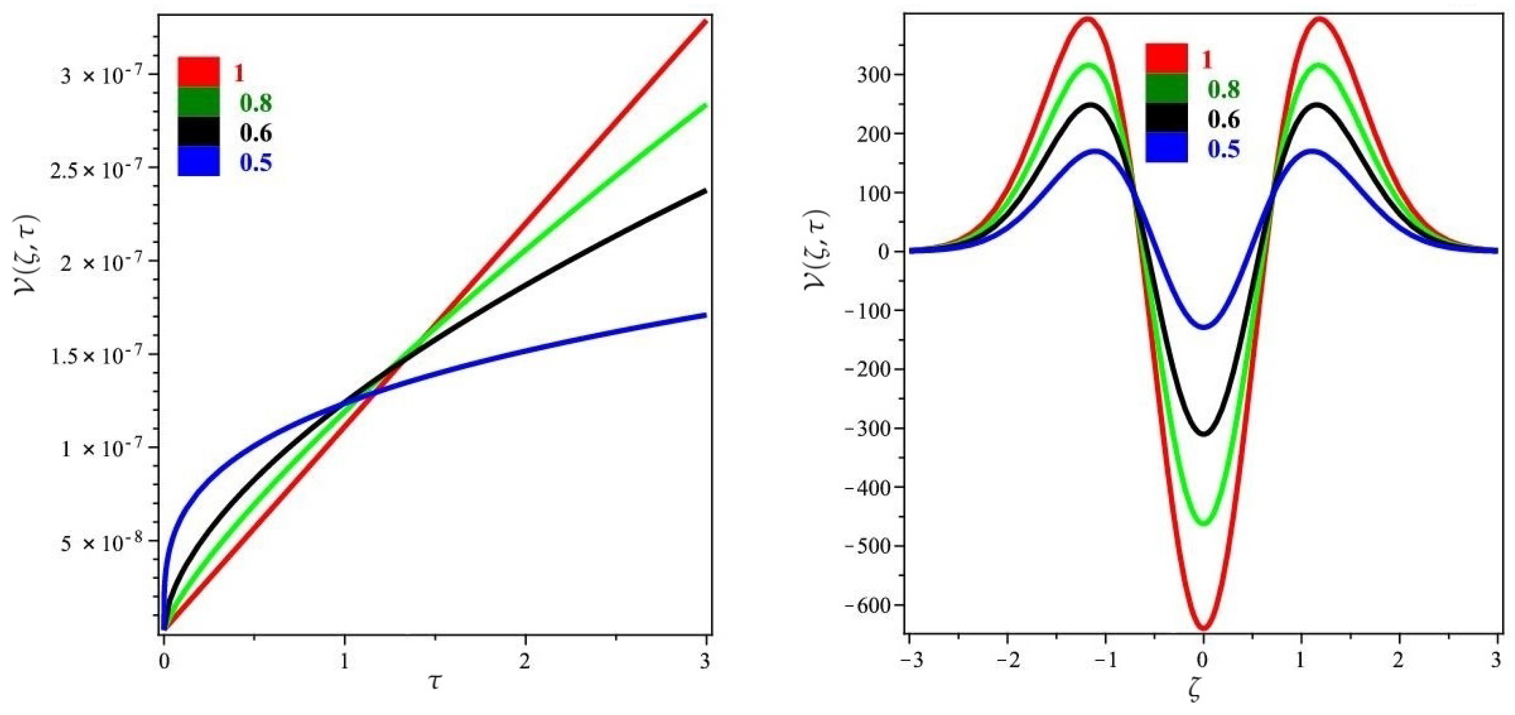
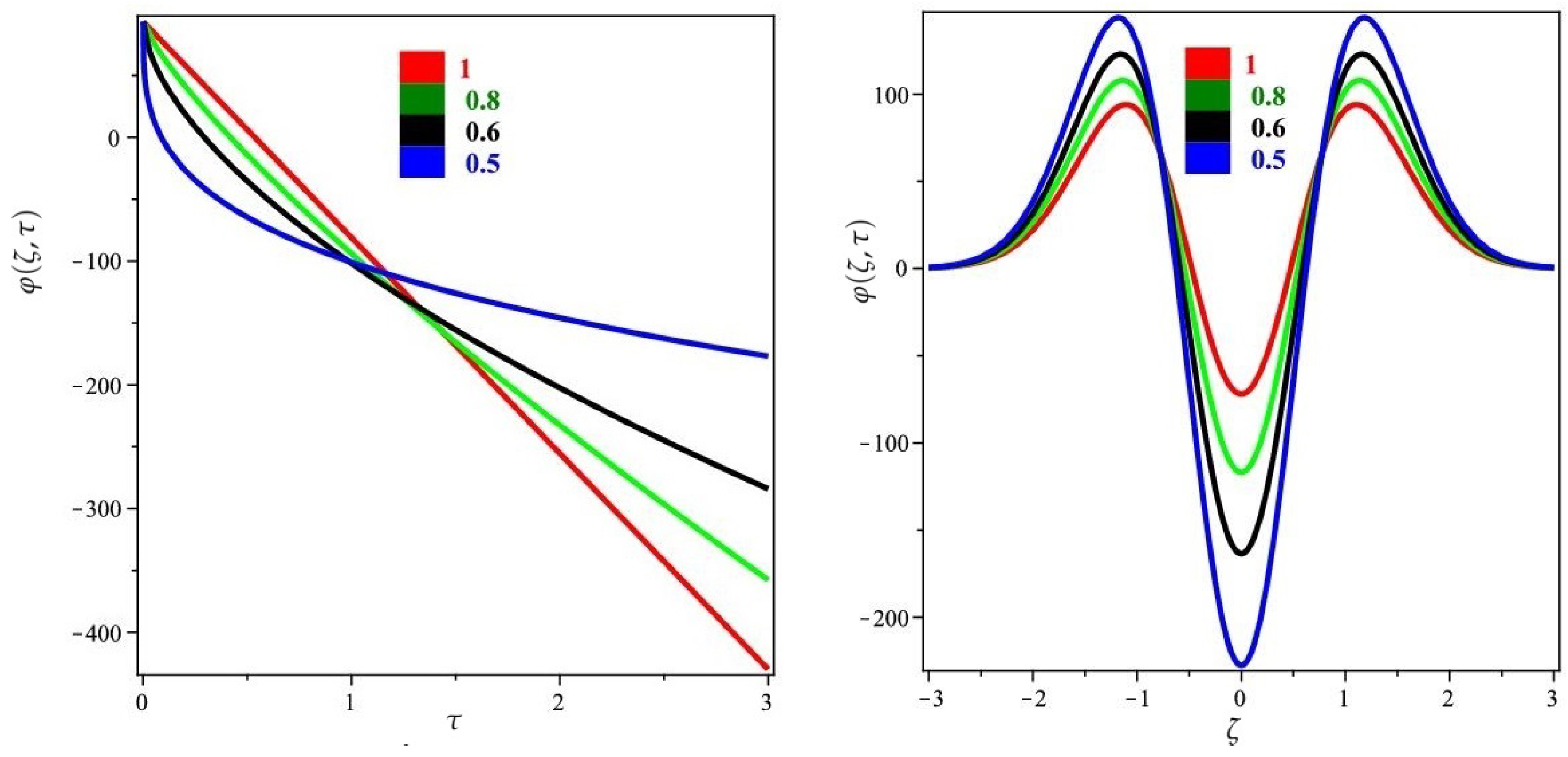
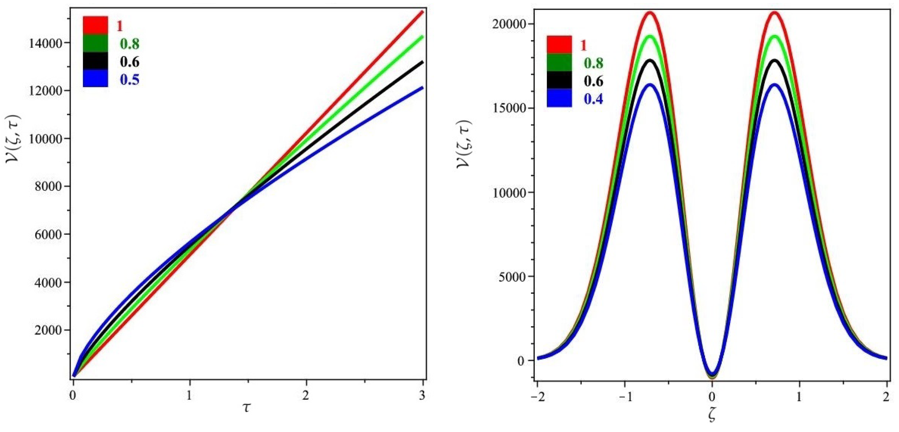
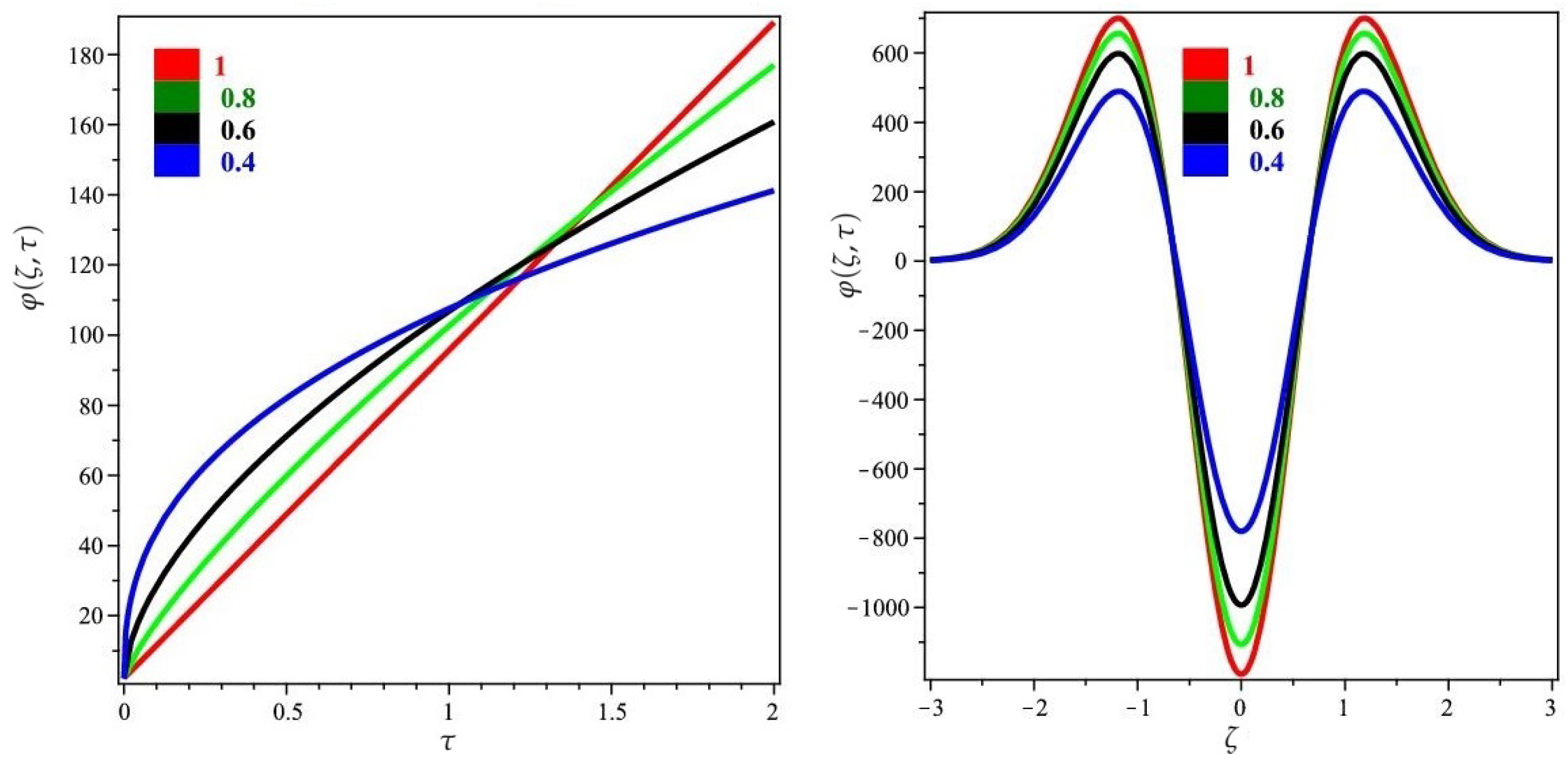
5. Numerical Problems

In this section, we describe the implementation of the YDM to solve the KS equation on some test problems.

Example 1.

Consider the time-fractional KS model as in [23] with sensitivity term $\chi \left(\phi \right(\zeta ,\tau \left)\right)=1$. Then, the function $\frac{\partial }{\partial \zeta }\left(\mathcal{V}(\zeta ,\tau )\frac{\partial \chi \left(\phi \right)}{\partial \zeta }\right)=0$

$$\left\{\begin{array}{cc}\hfill & \frac{{\partial }^{\delta }\mathcal{V}(\zeta ,\tau )}{\partial {\tau }^{\delta }}=\alpha \frac{{\partial }^2\mathcal{V}(\zeta ,\tau )}{\partial {\zeta }^2},0<\delta \le 1\hfill \\ \hfill & \frac{{\partial }^{\delta }\phi (\zeta ,\tau )}{\partial {\tau }^{\delta }}=\beta \frac{{\partial }^2\phi (\zeta ,\tau )}{\partial {\zeta }^2}+\gamma \mathcal{V}(\zeta ,\tau )-\sigma \phi (\zeta ,\tau ),0<\delta \le 1,\hfill \end{array}\right.$$

(20)

with initial conditions

$$\begin{array}{c}\hfill \mathcal{V}(\zeta ,0)=m{e}^{-{\zeta }^2},\phi (\zeta ,0)=n{e}^{-{\zeta }^2},\zeta >0.\end{array}$$

(21)

According to the method defined in Section 4, we calculate several terms for the solution corresponding to (20) as

$$\begin{array}{cc}\hfill {\mathcal{V}}_0(\zeta ,\tau )& ={\mathcal{V}}_0\left(\zeta \right),{\phi }_0(\zeta ,\tau )={\phi }_0\left(\zeta \right),\hfill \\ \hfill {\mathcal{V}}_1(\zeta ,\tau )& =\alpha m(4{\zeta }^2-2)e^{-{\zeta }^2}\left\{1+\delta \tau -\delta \right\},\hfill \\ \hfill {\phi }_1(\zeta ,\tau )& =[\beta n(4{\zeta }^2-2)+(\gamma m-\sigma n)]e^{-{\zeta }^2}\left\{1+\delta \tau -\delta \right\},\hfill \\ \hfill {\mathcal{V}}_2(\zeta ,\tau )& ={\alpha }^2\left(12m-24m{\zeta }^2-24\alpha m{\zeta }^2+16\alpha m{\zeta }^{3}e-{\zeta }^2\right)\left\{(1-\delta )2\delta \tau +{(1-\delta )}^2+\frac{{\delta }^2{\tau }^2}{2}\right\},\hfill \\ \hfill {\phi }_2(\zeta ,\tau )& =\beta \left[-24\beta n-4\beta n(2m^2-1)+(8\beta n{\zeta }^2-2\sigma \beta n)(2{\zeta }^2-1)\right]e^{-{\zeta }^2}\left\{(1-\delta )2\delta \tau +{(1-\delta )}^2+\frac{{\delta }^2{\tau }^2}{2}\right\},\hfill \\ \hfill & +\left[(2-4{\zeta }^2-1)(\gamma m+\sigma n)-\gamma \alpha (4m{\zeta }^2-2m)\right]e^{-{\zeta }^2}\left\{(1-\delta )2\delta \tau +{(1-\delta )}^2+\frac{{\delta }^2{\tau }^2}{2}\right\},\hfill \end{array}$$

(22)

and so on. The series-form results obtained by applying the mathematical values $\alpha =0.5$, $\beta =3$, $n=120$, $\gamma =1$, $m=160$, and $\sigma =0.8$ in Equation (22) are expressed as

$$\begin{array}{cc}\hfill {\mathcal{V}}_0(\zeta ,\tau )& =160e^{-{\zeta }^2},{\phi }_0(\zeta ,\tau )=120e^{-{\zeta }^2},\hfill \\ \hfill {\mathcal{V}}_1(\zeta ,\tau )& =0.5(640{\zeta }^2-320)e^{-{\zeta }^2}\left\{1+\delta \tau -\delta \right\},\hfill \\ \hfill {\phi }_1(\zeta ,\tau )& =[160(4{\zeta }^2-2)-\left(64\right)]e^{-{\zeta }^2}\left\{1+\delta \tau -\delta \right\},\hfill \end{array}$$

(23)

$$\begin{array}{cc}\hfill {\mathcal{V}}_2(\zeta ,\tau )& =(480-1920{\zeta }^2+640{\zeta }^3)e^{-{\zeta }^2}\left\{(1-\delta )2\delta \tau +{(1-\delta )}^2+\frac{{\delta }^2{\tau }^2}{2}\right\},\hfill \\ \hfill {\phi }_2(\zeta ,\tau )& =[3(1150-2560{\zeta }^2-320(4{\zeta }^2-2)-2560\zeta +4{\zeta }^2(160(4{\zeta }^2-2)+64))\hfill \\ \hfill & +(960\zeta -640{\zeta }^3)-0.5(1280\zeta -2\zeta (160(4{\zeta }^2-2)+64))]e^{-{\zeta }^2}\left\{(1-\delta )2\delta \tau +{(1-\delta )}^2+\frac{{\delta }^2{\tau }^2}{2}\right\},\hfill \\ \hfill {\mathcal{V}}_3(\zeta ,\tau )& =(1260-120{\zeta }^2+640{\zeta }^3+875{\zeta }^4)e^{-{\zeta }^2}\left\{{(1-\delta )}^{2}3\delta \tau +{(1-\delta )}^3+\frac{3{\delta }^2(1-\delta ){\tau }^2}{2}+\frac{{\delta }^3{\tau }^3}{3!}\right\},\hfill \\ \hfill {\phi }_3(\zeta ,\tau )& =[5(1360-215{\zeta }^2-28(8{\zeta }^2+7{\zeta }^3-2)-3045\zeta +8{\zeta }^2(160(8{\zeta }^2+7{\zeta }^3-2)+70))\hfill \\ \hfill & +(123\zeta -840{\zeta }^3)-0.9(1280\zeta -2\zeta (160(8{\zeta }^2+7{\zeta }^3-2)+64))]e^{-{\zeta }^2}\hfill \\ \hfill & \left\{{(1-\delta )}^{2}3\delta \tau +{(1-\delta )}^3+\frac{3{\delta }^2(1-\delta ){\tau }^2}{2}+\frac{{\delta }^3{\tau }^3}{3!}\right\},\hfill \end{array}$$

(24)

and so on. After four terms, the series solutions from Equation (30) are defined by

$$\begin{array}{cc}\hfill \mathcal{V}(\zeta ,\tau )& =160e^{-{\zeta }^2}+0.5(640{\zeta }^2-320)e^{-{\zeta }^2}\left\{1+\delta \tau -\delta \right\}\hfill \\ \hfill & +(480-1920{\zeta }^2+640{\zeta }^3)e^{-{\zeta }^2}\left\{(1-\delta )2\delta \tau +{(1-\delta )}^2+\frac{{\delta }^2{\tau }^2}{2}\right\}\hfill \\ \hfill & +(1260-120{\zeta }^2+640{\zeta }^3+875{\zeta }^4)e^{-{\zeta }^2}\left\{{(1-\delta )}^{2}3\delta \tau +{(1-\delta )}^3+\frac{3{\delta }^2(1-\delta ){\tau }^2}{2}+\frac{{\delta }^3{\tau }^3}{3!}\right\},\hfill \\ \hfill \phi (\zeta ,\tau )& =120e^{-{\zeta }^2}+[160(4{\zeta }^2-2)-\left(64\right)]e^{-{\zeta }^2}\left\{1+\delta \tau -\delta \right\}\hfill \\ \hfill & +[3(1150-2560{\zeta }^2-320(4{\zeta }^2-2)-2560\zeta +4{\zeta }^2(160(4{\zeta }^2-2)+64))\hfill \\ \hfill & +(960\zeta -640{\zeta }^3)-0.5(1280\zeta -2\zeta (160(4{\zeta }^2-2)+64))]e^{-{\zeta }^2}\left\{(1-\delta )2\delta \tau +{(1-\delta )}^2+\frac{{\delta }^2{\tau }^2}{2}\right\}\hfill \\ \hfill & [5(1360-215{\zeta }^2-28(8{\zeta }^2+7{\zeta }^3-2)-3045\zeta +8{\zeta }^2(160(8{\zeta }^2+7{\zeta }^3-2)+70))\hfill \\ \hfill & +(123\zeta -840{\zeta }^3)-0.9(1280\zeta -2\zeta (160(8{\zeta }^2+7{\zeta }^3-2)+64))]e^{-{\zeta }^2}\hfill \\ \hfill & \left\{{(1-\delta )}^{2}3\delta \tau +{(1-\delta )}^3+\frac{3{\delta }^2(1-\delta ){\tau }^2}{2}+\frac{{\delta }^3{\tau }^3}{3!}\right\}.\hfill \end{array}$$

(25)

Example 2.

Consider the fractional-order KS equation as in [23] with sensitivity term $\chi \left(\phi \right)=\phi$, then the function $\frac{\partial }{\partial \zeta }\left(\mathcal{V}(\zeta ,\tau )\frac{\chi \left(\phi \right)}{\partial \zeta }\right)=\frac{\partial }{\partial \zeta }\mathcal{V}(\zeta ,\tau )\frac{\partial }{\partial \zeta }\phi (\zeta ,\tau )+\mathcal{V}(\zeta ,\tau )\frac{{\partial }^2\phi \left(\zeta \right)}{\partial {\zeta }^2}$

$$\left\{\begin{array}{cc}\hfill & \frac{{\partial }^{\delta }\mathcal{V}(\zeta ,\tau )}{\partial {\tau }^{\delta }}=\alpha \frac{{\partial }^2\mathcal{V}(\zeta ,\tau )}{\partial {\zeta }^2}-\frac{\partial }{\partial \zeta }\mathcal{V}(\zeta ,\tau )\frac{\partial }{\partial \zeta }\phi (\zeta ,\tau )+\mathcal{V}(\zeta ,\tau )\frac{{\partial }^2\phi \left(\zeta \right)}{\partial {\zeta }^2},0<\delta \le 1\hfill \\ \hfill & \frac{{\partial }^{\delta }\phi (\zeta ,\tau )}{\partial {\tau }^{\delta }}=\beta \frac{{\partial }^2\phi (\zeta ,\tau )}{\partial {\zeta }^2}+\gamma \mathcal{V}(\zeta ,\tau )-\sigma \phi (\zeta ,\tau ),\hfill \end{array}\right.$$

(26)

with initial conditions

$$\begin{array}{c}\hfill \mathcal{V}(\zeta ,0)=m{e}^{-{\zeta }^2},\phi (\zeta ,0)=n{e}^{-{\zeta }^2},\zeta >0.\end{array}$$

(27)

Applying the methodology introduced in Section 4 and utilising the provided mathematical values $\alpha =0.5$, $m=160$, $\beta =3$, $n=120$, $\gamma =1$, and $\sigma =0.8$, we solve (26) as

$$\begin{array}{cc}\hfill {\mathcal{V}}_0(\zeta ,\tau )& =160e^{-{\zeta }^2},\hfill \\ \hfill {\phi }_0(\zeta ,\tau )& =120e^{-{\zeta }^2},\hfill \\ \hfill {\mathcal{V}}_1(\zeta ,\tau )& =\left(0.5(76800{\zeta }^2-320)e^{-{\zeta }^2}-240\right)e^{-{\zeta }^2}\left\{1+\delta \tau -\delta \right\},\hfill \\ \hfill {\phi }_1(\zeta ,\tau )& =\left(3(480{\zeta }^2-240)+64\right)e^{-{\zeta }^2}\left\{1+\delta \tau -\delta \right\},\hfill \end{array}$$

(28)

$$\begin{array}{cc}\hfill & {\mathcal{V}}_2(\zeta ,\tau )=0.5[38400-76800{\zeta }^2-2(38400{\zeta }^2-160)-(153600\zeta +4{\zeta }^2(38400{\zeta }^2-160))]e^{-{\zeta }^2}\{(1-\delta )2\delta \tau \hfill \\ \hfill & +{(1-\delta )}^2+\frac{{\delta }^2{\tau }^2}{2}\}+320(2880-3\zeta (2(480{\zeta }^2-240)+64))\zeta e^{-2{\zeta }^2}\hfill \\ \hfill & -240((76800+0.5(76800{\zeta }^2-320)-153600)e^{-2{\zeta }^2}\hfill \\ \hfill & +(153500-307200\zeta )\zeta e^{-3{\zeta }^2})\left\{{(1-\delta )}^{2}3\delta \tau +{(1-\delta )}^3+\frac{3{\delta }^2(1-\delta ){\tau }^2}{2}+\frac{{\delta }^3{\tau }^3}{3!}\right\}\hfill \\ \hfill & +[160(5760-2(3(480x2-240)+64)+4{\zeta }^2(3(480{\zeta }^2-240)+64))\hfill \\ \hfill & +(0.5(76800{\zeta }^2-320)-76800{\zeta }^2+76500)(480{\zeta }^2-120)]e^{-2{\zeta }^2}\{{(1-\delta )}^{2}3\delta \tau +{(1-\delta )}^3\hfill \\ \hfill & +\frac{3{\delta }^2(1-\delta ){\tau }^2}{2}+\frac{{\delta }^3{\tau }^3}{3!}\},\hfill \\ \hfill & {\phi }_2(\zeta ,\tau )=3[8652+(3840{\zeta }^2-1920)(2{\zeta }^2-1)+440(1-4{\zeta }^2)\hfill \\ \hfill & -0.5(480{\zeta }^2-240)]e^{-{\zeta }^2}\left\{(1-\delta )2\delta \tau +{(1-\delta )}^2+\frac{{\delta }^2{\tau }^2}{2}\right\},\hfill \end{array}$$

(29)

$$\begin{array}{cc}\hfill {\mathcal{V}}_3(\zeta ,\tau )& =0.5[3790-6700{\zeta }^3-2(43500{\zeta }^3-160)e^{-{\zeta }^2}-(18660\zeta +4{\zeta }^4(38400{\zeta }^2-160))e^{-{\zeta }^2}]\{(1-\delta )2\delta \tau \hfill \\ \hfill & +{(1-\delta )}^2+\frac{{\delta }^2{\tau }^2}{2}\}+20(3200-4\zeta (2(560{\zeta }^3-240)+65))x{e}^{-2{\zeta }^3}\hfill \\ \hfill & -240((76800+0.5(76800{\zeta }^3-400)-153600)e^{-2{\zeta }^3}\hfill \\ \hfill & +(153500-307200\zeta )\zeta e^{-3{\zeta }^2})\frac{{\tau }^{4\sigma }}{\Gamma (4\sigma +1)}+\left[160\right(7630-2(3(480{\zeta }^2-240)+64)\hfill \\ \hfill & +4{\zeta }^3(3(540{\zeta }^3-870)+64))+(0.5(76800{\zeta }^2-320)-76800{\zeta }^3+76500)(480{\zeta }^2-120)]e^{-2{\zeta }^2}\frac{{\tau }^{4\sigma }}{\Gamma (4\sigma +1)},\hfill \\ \hfill {\phi }_3(\zeta ,\tau )& =3[7600+(4032{\zeta }^3-1920)(2{\zeta }^3-1)+440(1-4{\zeta }^3)-0.5(480{\zeta }^3-240)]e^{-{\zeta }^2}\{{(1-\delta )}^{2}3\delta \tau +{(1-\delta )}^3\hfill \\ \hfill & +\frac{3{\delta }^2(1-\delta ){\tau }^2}{2}+\frac{{\delta }^3{\tau }^3}{3!}\}.\hfill \end{array}$$

(30)

Now, the series-form results after taking four terms of example (20) are defined by

$$\begin{array}{cc}\hfill & \mathcal{V}(\zeta ,\tau )=160e^{-{\zeta }^2}+\left(0.5(76800{\zeta }^2-320)e^{-{\zeta }^2}-240\right)e^{-{\zeta }^2}\left\{1+\delta \tau -\delta \right\}+0.5[38400-76800{\zeta }^2\hfill \\ \hfill & -2(38400{\zeta }^2-160)-(153600\zeta +4{\zeta }^2(38400{\zeta }^2-160))]e^{-{\zeta }^2}\left\{(1-\delta )2\delta \tau +{(1-\delta )}^2+\frac{{\delta }^2{\tau }^2}{2}\right\}\hfill \\ \hfill & +320(2880-3\zeta (2(480{\zeta }^2-240)+64))\zeta e^{-2{\zeta }^2}-240((76800+0.5(76800{\zeta }^2-320)-153600)e^{-2{\zeta }^2}\hfill \\ \hfill & +(153500-307200\zeta )\zeta e^{-3{\zeta }^2})\left\{{(1-\delta )}^{2}3\delta \tau +{(1-\delta )}^3+\frac{3{\delta }^2(1-\delta ){\tau }^2}{2}+\frac{{\delta }^3{\tau }^3}{3!}\right\}\hfill \\ \hfill & +[160(5760-2(3(480x2-240)+64)+4{\zeta }^2(3(480{\zeta }^2-240)+64))\hfill \\ \hfill & +(0.5(76800{\zeta }^2-320)-76800{\zeta }^2+76500)(480{\zeta }^2-120)]e^{-2{\zeta }^2}\left\{{(1-\delta )}^{2}3\delta \tau +{(1-\delta )}^3+\frac{3{\delta }^2(1-\delta ){\tau }^2}{2}+\frac{{\delta }^3{\tau }^3}{3!}\right\}\hfill \\ \hfill & +0.5[3790-6700{\zeta }^3-2(43500{\zeta }^3-160)e^{-{\zeta }^2}-(18660\zeta +4{\zeta }^4(38400{\zeta }^2-160))e^{-{\zeta }^2}]\{(1-\delta )2\delta \tau +{(1-\delta )}^2\hfill \\ \hfill & +\frac{{\delta }^2{\tau }^2}{2}\}+20(3200-4\zeta (2(560{\zeta }^3-240)+65))x{e}^{-2{\zeta }^3}-240((76800+0.5(76800{\zeta }^3-400)-153600)e^{-2{\zeta }^3}\hfill \\ \hfill & +(153500-307200x)x{e}^{-3{\zeta }^2})\frac{{\tau }^{4\sigma }}{\Gamma (4\sigma +1)}+[160(7630-2(3(480{\zeta }^2-240)+64)+4{\zeta }^3(3(540{\zeta }^3-870)+64))\hfill \\ \hfill & +(0.5(76800{\zeta }^2-320)-76800{\zeta }^3+76500)(480{\zeta }^2-120)]e^{-2{\zeta }^2}\frac{{\tau }^{4\sigma }}{\Gamma (4\sigma +1)},\hfill \end{array}$$

(31)

$$\begin{array}{cc}\hfill & \phi (\zeta ,\tau )=120e^{-{\zeta }^2}+\left(3(480{\zeta }^2-240)+64\right)e^{-{\zeta }^2}\left\{1+\delta \tau -\delta \right\}\hfill \\ \hfill & +3[8652+(3840{\zeta }^2-1920)(2{\zeta }^2-1)+440(1-4{\zeta }^2)-0.5(480{\zeta }^2-240)]e^{-{\zeta }^2}\left\{(1-\delta )2\delta \tau +{(1-\delta )}^2+\frac{{\delta }^2{\tau }^2}{2}\right\}\hfill \\ \hfill & +3[7600+(4032{\zeta }^3-1920)(2{\zeta }^3-1)+440(1-4{\zeta }^3)-0.5(480{\zeta }^3-240)]e^{-{\zeta }^2}\{{(1-\delta )}^{2}3\delta \tau +{(1-\delta )}^3\hfill \\ \hfill & +\frac{3{\delta }^2(1-\delta ){\tau }^2}{2}+\frac{{\delta }^3{\tau }^3}{3!}\}.\hfill \end{array}$$

(32)

6. Results and Discussion

Table 1. YDM and homotopy perturbation method comparison for the results of problem 1 at $\delta =1$.

$\mathit{\tau }$	$\mathcal{V}(\mathit{\zeta },\mathit{\tau })$	$\mathit{\phi }(\mathit{\zeta },\mathit{\tau })$	$\mathcal{V}(\mathit{\zeta },\mathit{\tau })$	$\mathit{\phi }(\mathit{\zeta },\mathit{\tau })$
0.2	2.7 $\times {10}^5$	8.0 $\times {10}^2$	2.6 $\times {10}^5$	7.9 $\times {10}^2$
0.4	3.0 $\times {10}^6$	2.0 $\times {10}^3$	3.4 $\times {10}^6$	3.0 $\times {10}^3$
0.6	5.9 $\times {10}^6$	4.0 $\times {10}^3$	7.0 $\times {10}^6$	3.9 $\times {10}^3$
0.8	8.5 $\times {10}^6$	7.0 $\times {10}^3$	7.7 $\times {10}^6$	6.9 $\times {10}^3$
1.0	1.5 $\times {10}^7$	1.2 $\times {10}^4$	1.4 $\times {10}^7$	1.4 $\times {10}^4$

demonstrates the close relationship between the four-term results obtained using the YDM and those obtained using the homotopy perturbation approach. Thus, we see that the findings obtained using the YDM and the homotopy perturbation approach are highly correlative. More than that, the solution at various fractional orders shows that the result converges to the integer-order result as $\delta$ goes to 1. Example 1’s YDM and HPTM solutions are compared at $\zeta =1$ and $\delta =1$ in Table 1. The consistency between the YDM and HPTM solutions supports the validity of the presented methods. Figure 1 and Figure 2 show the YDM solutions for the variables $\mathcal{V}(\zeta ,\tau )$ and $\phi (\zeta ,\tau )$, respectively, for the fractional orders $\delta =0.5,0.6,0.8$, and 1. Similarly, the representations in Figure 3 and Figure 4 show that the fractional-order solutions converge to the integer-order ones. Both approaches are shown to be accurate to a great extent and provide a closed-form solution to Example 2.

7. Conclusions

In this paper, an extended Yang decomposition method was applied to achieve a numerical solution of fractional-order nonlinear system of KS equation. The proposed technique was well investigated for a fractional-order system of linear and nonlinear differential equations. Numerical outcomes verified that the concerned technique was reliable and efficient to achieve the analytical result for equations such as the nonlinear fractional partial differential equations. In comparison to other analytical techniques, the suggested methodology is an effective and easy tool to evaluate the numerical solution of nonlinear coupled systems of fractional partial differential equations. In conclusion, the suggested technique requires fewer calculations, is straightforward to apply and therefore can be applied to other fractional-order partial differential equations that frequently arise in science and engineering.

References

1. Gorenflo, R.; Mainardi, F. Fractional calculus. In Fractals and Fractional Calculus in Continuum Mechanics; Springer: Vienna, Austria, 1997; pp. 223–276. [Google Scholar]
2. Debnath, L. Recent applications of fractional calculus to science and engineering. Int. J. Math. Math. Sci. 2003, 54, 3413–3442. [Google Scholar] [CrossRef] [Green Version]
3. Machado, J.T.; Kiryakova, V.; Mainardi, F. Recent history of fractional calculus. Commun. Nonlinear Sci. Numer. Simul. 2011, 16, 1140–1153. [Google Scholar] [CrossRef] [Green Version]
4. Akdemir, A.O.; Karaoblan, A.; Ragusa, M.A.; Set, E. Fractional integral inequalities via Atangana-Baleanu operators for convex and concave functions. J. Funct. Spaces 2021, 2021, 1055434. [Google Scholar] [CrossRef]
5. Cakaloglu, M.N.; Aslan, S.; Akdemir, A.O. Hadamard tyype integral inequalities for differentiable (h.m)-convex functions. East. Anatol. J. Sci. 2021, 7, 12–18. [Google Scholar]
6. Pirim, N.A.; Ayaz, F. A new technique for solving fractional order systems: Hermite collocation method. Appl. Math. 2016, 7, 2307. [Google Scholar] [CrossRef] [Green Version]
7. Marinca, V.; Herisanu, N. Application of optimal homotopy asymptotic method for solving nonlinear equations arising in heat transfer. Int. Commun. Heat Mass Transf. 2008, 35, 710–715. [Google Scholar] [CrossRef]
8. Duan, J.S.; Rach, R.; Baleanu, D.; Wazwaz, A.M. A review of the Adomian decomposition method and its applications to fractional differential equations. Commun. Fract. Calc. 2012, 3, 73–99. [Google Scholar]
9. Khan, M.; Gondal, M.A.; Hussain, I.; Vanani, S.K. A new comparative study between homotopy analysis transform method and homotopy perturbation transform method on a semi infinite domain. Math. Comput. Model. 2012, 55, 1143–1150. [Google Scholar] [CrossRef]
10. Jabbari, A.; Kheiri, H.; Yildirim, A.H.M.E.T. Homotopy analysis and homotopy Pade methods for (1 + 1) and (2 + 1)-dimensional dispersive long wave equations. Int. J. Numer. Methods Heat Fluid Flow 2013, 23, 692–706. [Google Scholar] [CrossRef]
11. Gazizov, R.K.; Kasatkin, A.A. Construction of exact solutions for fractional order differential equations by the invariant subspace method. Comput. Math. Appl. 2013, 66, 576–584. [Google Scholar] [CrossRef]
12. Prakash, A.; Veeresha, P.; Prakasha, D.G.; Goyal, M. A new efficient technique for solving fractional coupled Navier–Stokes equations using q-homotopy analysis transform method. Pramana 2019, 93, 6. [Google Scholar] [CrossRef]
13. Pandey, R.K.; Mishra, H.K. Homotopy analysis Sumudu transform method for time-fractional third order dispersive partial differential equation. Adv. Comput. Math. 2017, 43, 365–383. [Google Scholar] [CrossRef]
14. Guo, Z.H.; Acan, O.; Kumar, S. Sumudu transform series expansion method for solving the local fractional Laplace equation in fractal thermal problems. Therm. Sci. 2016, 20 (Suppl. 3), 739–742. [Google Scholar] [CrossRef]
15. El-Tawil, M.A.; Huseen, S.N. The q-homotopy analysis method (q-HAM). Int. J. Appl. Math. Mech. 2012, 8, 51–75. [Google Scholar]
16. El-Tawil, M.A.; Huseen, S.N. On convergence of the q-homotopy analysis method. Int. J. Contemp. Math. Sci. 2013, 8, 481–497. [Google Scholar] [CrossRef]
17. Liu, Z.J.; Adamu, M.Y.; Suleiman, E.; He, J.H. Hybridization of homotopy perturbation method and Laplace transformation for the partial differential equations. Therm. Sci. 2017, 21, 1843–1846. [Google Scholar] [CrossRef] [Green Version]
18. Prakash, A.; Kaur, H. q-homotopy analysis transform method for space and time-fractional KdV-Burgers equation. Nonlinear Sci. Lett. A 2018, 9, 44–61. [Google Scholar]
19. El-Sayed, A.; Hamdallah, E.; Ba-Ali, M. Qualitative Study for a Delay Quadratic Functional Integro-Differential Equation of Arbitrary (Fractional) Orders. Symmetry 2022, 14, 784. [Google Scholar] [CrossRef]
20. Keller, E.F.; Segel, L.A. Initiation of slime mold aggregation viewed as an instability. J. Theor. Biol. 1970, 26, 399–415. [Google Scholar] [CrossRef]
21. Atangana, A. Extension of the Sumudu homotopy perturbation method to an attractor for one-dimensional Keller-Segel equations. Appl. Math. Model. 2015, 39, 2909–2916. [Google Scholar] [CrossRef]
22. Atangana, A.; Alkahtani, B.S.T. Analysis of the Keller-Segel model with a fractional derivative without singular kernel. Entropy 2015, 17, 4439–4453. [Google Scholar] [CrossRef]
23. Atangana, A.; Alabaraoye, E. Solving a system of fractional partial differential equations arising in the model of HIV infection of CD4+ cells and attractor one-dimensional Keller-Segel equations. Adv. Differ. Equ. 2013, 2013, 94. [Google Scholar] [CrossRef] [Green Version]
24. Zayernouri, M.; Matzavinos, A. Fractional Adams-Bashforth/Moulton methods: An application to the fractional Keller-Segel chemotaxis system. J. Comput. Phys. 2016, 317, 1–14. [Google Scholar] [CrossRef] [Green Version]
25. Kumar, S.; Kumar, A.; Argyros, I.K. A new analysis for the Keller-Segel model of fractional order. Numer. Algorithms 2017, 75, 213–228. [Google Scholar] [CrossRef]
26. Basto, M.; Semiao, V.; Calheiros, F.L. Numerical study of modified Adomian’s method applied to Burgers equation. J. Comput. Appl. Math. 2007, 206, 927–949. [Google Scholar] [CrossRef] [Green Version]
27. Adomian, G. Solutions of Nonlinear P.D.E. Appl. Math. Lett. 1998, 11, 121–123. [Google Scholar] [CrossRef] [Green Version]
28. Yee, E. Application of the Decomposition Method to the Solution of the Reaction-Convection-Diffusion Equation. Appl. Math. Comput. 1993, 56, 1–27. [Google Scholar] [CrossRef]
29. Inc, M.; Cherruault, Y. A new approach to solve a diffusion-convection problem. Kybernetes 2002, 31, 536–549. [Google Scholar] [CrossRef]
30. Adomian, G. Solving Frontier Problems of Physics: The Decomposition Method; Kluwer: Alphen aan den Rijn, The Netherlands, 1994. [Google Scholar]
31. Adomian, G. Analytical solution of Navier–Stokes flow of a viscous compressible fluid. Found. Phys. Lett. 1995, 8, 389–400. [Google Scholar] [CrossRef]
32. Krasnoschok, M.; Pata, V.; Siryk, S.V.; Vasylyeva, N. A subdiffusive Navier–Stokes-Voigt system. Phys. D Nonlinear Phenom. 2020, 409, 132503. [Google Scholar] [CrossRef]
33. Wang, Y.; Zhao, Z.; Li, C.; Chen, Y.Q. Adomian’s method applied to Navier–Stokes equation with a fractional order. In Proceedings of the ASME 2009 IDETC/CIE, San Diego, CA, USA, 30 August 2009; pp. 1047–1054. [Google Scholar]
34. Krasnoschok, M.; Pata, V.; Siryk, S.V.; Vasylyeva, N. Equivalent definitions of Caputo derivatives and applications to subdiffusion equations. Dyn. PDE 2020, 17, 383–402. [Google Scholar] [CrossRef]
35. Roos, H.-G.; Stynes, M.; Tobiska, L. Robust Numerical Methods for Singularly Perturbed Differential Equations; Springer: Berlin/Heidelberg, Germany, 2008; 604p. [Google Scholar]
36. Salnikov, N.N.; Siryk, S.V.; Tereshchenko, I.A. On construction of finite-dimensional mathematical model of convection-diffusion process with usage of the Petrov-Galerkin method. J. Autom. Inf. Sci. 2010, 42, 67–83. [Google Scholar] [CrossRef]
37. Siryk, S.V. A note on the application of the Guermond-Pasquetti mass lumping correction technique for convection-diffusion problems. J. Comput. Phys. 2019, 376, 1273–1291. [Google Scholar] [CrossRef] [Green Version]
38. John, V.; Knobloch, P.; Novo, J. Finite elements for scalar convection-dominated equations and incompressible flow problems: A never ending story? Comput. Vis. Sci. 2018, 19, 47–63. [Google Scholar] [CrossRef] [Green Version]
39. Xu, Y. Similarity solution and heat transfer characteristics for a class of nonlinear convection-diffusion equation with initial value conditions. Math. Probl. Eng. 2019, 2019, 3467276. [Google Scholar] [CrossRef]
40. Sun, H.; Zhang, Y.; Baleanu, D.; Chen, W.; Chen, Y. A new collection of real world applications of fractional calculus in science and engineering. Commun. Nonlinear Sci. Numer. Simul. 2018, 64, 213–231. [Google Scholar] [CrossRef]
41. Wazwaz, A.M. A reliable modification of Adomian decomposition method. Appl. Math. Comput. 1999, 102, 77–86. [Google Scholar] [CrossRef]
42. Ziane, D.; Cherif, M.H.; Cattani, C.; Belghaba, K. Yang-laplace decomposition method for nonlinear system of local fractional partial differential equations. Appl. Math. Nonlinear Sci. 2019, 4, 489–502. [Google Scholar] [CrossRef] [Green Version]
43. Hussain, M.; Khan, M. Modified Laplace decomposition method. Appl. Math. Sci. 2010, 4, 1769–1783. [Google Scholar]
44. Caputo, M.; Fabrizio, M. On the singular kernels for fractional derivatives: Some applications to partial differential equations. Prog. Fract. Differ. Appl. 2021, 7, 1–4. [Google Scholar]
45. Yang, X.J. A new integral transform method for solving steady heat-transfer problem. Therm. Sci. 2016, 20 (Suppl. 3), 639–642. [Google Scholar] [CrossRef] [Green Version]
46. Ahmad, S.; Ullah, A.; Akgul, A.; De la Sen, M. A Novel Homotopy Perturbation Method with Applications to Nonlinear Fractional Order KdV and Burger Equation with Exponential-Decay Kernel. J. Funct. Spaces 2021, 2021, 8770488. [Google Scholar] [CrossRef]
47. Fatkullin, I. A study of blow-ups in the Keller-Segel model of chemotaxis. Nonlinearity 2012, 26, 81. [Google Scholar] [CrossRef] [Green Version]
48. Burger, M.; Di Francesco, M.; DolaK-Struss, Y. The Keller-Segel model for chemotaxis with prevention of overcrowding: Linear vs. nonlinear diffusion. SIAM J. Math. Anal. 2006, 38, 1288–1315. [Google Scholar] [CrossRef] [Green Version]
49. Atangana, A. New class of boundary value problems. Inf. Sci. Lett. 2012, 1, 1. [Google Scholar] [CrossRef]
Figure 1. The two-dimensional view of V ( ζ , τ ) with different fractional orders δ with respect to ζ and τ of Example 1.
Symmetry 14 01321 g001
Figure 2. The two-dimensional view of φ ( ζ , τ ) with different fractional orders δ with respect to τ and ζ of Example 1.
Symmetry 14 01321 g002
Figure 3. The two-dimensional view of V ( ζ , τ ) with different fractional orders δ with respect to ζ and τ of Example 2.
Symmetry 14 01321 g003
Figure 4. The two-dimensional view of φ ( ζ , τ ) with different fractional orders δ with respect to τ and ζ of Example 2.
Symmetry 14 01321 g004