Article

3D Localization Method of Partial Discharge in Air-Insulated Substation Based on Improved Particle Swarm Optimization Algorithm

School of Electrical and Mechanical Engineering, Pingdingshan University, Pingdingshan 467000, China
*
Author to whom correspondence should be addressed.
Symmetry 2022, 14(6), 1241; https://doi.org/10.3390/sym14061241
Submission received: 23 May 2022 / Revised: 8 June 2022 / Accepted: 11 June 2022 / Published: 15 June 2022
(This article belongs to the Special Issue Meta-Heuristics for Manufacturing Systems Optimization)

Abstract

:
Partial discharge (PD) localization in an air-insulated substation (AIS) can be used to assess insulation conditions efficiently. Many localization methods have been reported during the past few years. However, the error of the localization results has been large or the localization algorithm too inefficient. The reason is that the localization equation set is nonlinear and non-symmetrical. In this paper, an improved particle swarm optimization (PSO) algorithm is proposed to improve the localization accuracy in 3D. Firstly, the proposed localization method is based on the symmetrical antenna array and the location error distribution is analyzed. Secondly, the objective function of PSO is constructed using the error distribution. Specifically, the 3D location target is divided into two steps—plane coordinates and height. The two targets are optimized respectively. To verify the method, a test is carried out by a prefabricated fault bushing in the laboratory to compare with the existing methods. According to the results, the localization error is 0.21 m, which can locate the PD source accurately. A complete calculation takes 42.29 s, and the efficiency is increased by 16.13 times under the same accuracy. The comparison results show that the proposed method can greatly improve the efficiency while ensuring accuracy.

1. Introduction

Partial discharge (PD) is a small discharge phenomenon occurring in insulating materials. With the development of PD, the discharge intensity will gradually increase. At the same time, it will lead to further deterioration of the insulating material. In severe cases, it will cause insulation breakdown [1,2,3]. The power equipment in open substations varies and is intensively placed. Insulation failure caused by partial discharge (PD) is particularly serious [4,5,6]. When the equipment operates for a long time, the detection of partial discharge becomes difficult [7]. The Ultra-High Frequency (UHF) method is widely used in the detection of PD, due to its advantages, such as high sensitivity, strong anti-interference ability, and non-contact measurement [8,9]. Based on the UHF method, whole-station PD location detection in the open substation can effectively improve the detection efficiency [10,11,12].
At the end of the 20th century, the British scholar PJ. Moore developed a PD localization device based on the UHF method. This method uses the vehicle-mounted method to realize the detection of the whole air-insulated substation (AIS) [13], and later adopts the installation of four antennas on the roof of the substation to locate the PD of the whole station [14]. Specifically, the method is based on the time difference of arrival (TDOA) algorithm for locating. Further, the method uses the four UHF signals collected synchronously to establish an equation set and obtains the coordinates of the PD source by solving the equation set. However, the equation set is nonlinear and non-symmetrical, and there is an error in the time delay. It is difficult to solve the equation set, leading to a large localization error. Usually, the localization results are azimuth or coordinates in the two-dimensional plane, and the error of the localization results is related to the attitude of the sensor array [14,15]. Study [16] proposes a method of using two antennas to locate the PD source, and its core algorithm is also the time difference of the arrival algorithm. According to the analysis of the current research results [17,18,19], the theoretically established equations have no solution due to errors in the time delay estimation. References [20,21,22] use the received signal strength indicator (RSSI) method, multiple signal classification (MUSIC) algorithm, angle of arrival (AOA) and other algorithms for locating, realizing two-dimensional azimuth localization. References [23,24] use a grid search algorithm to search the space to realize the three-dimensional localization of the PD source. The efficiency of this algorithm is greatly affected by the size of the search grid and shows the disadvantage of excessive calculation. The localization error of reference [24] is 0.35 m, while the size of the entire space is 0.8 m × 1 m × 0.3 m. Reference [25] uses a particle swarm optimization (PSO) algorithm to locate PD sources of substations in 3D. With a minimum error of 1.59 m, it is still difficult to accurately obtain PD equipment in substations. Reference [26] adopts the localization method of multi-point measurement combined with error probability to achieve three-dimensional localization. The accuracy of this method is high, and the maximum error is 0.27 m in the substation. The method contains two steps. Firstly, the azimuths and elevation angles between the PD source and each measuring point are calculated by the PSO algorithm. Secondly, the intersection coordinates of all azimuth and pitch angles are calculated by the error probability algorithm, which is the positioning result. Apparently, the whole process includes multiple PSO algorithms and one error probability algorithm, which is overly complicated. To sum up, most of the currently reported substation PD localization methods achieve 2D localization. However, the 3D localization method cannot avoid large localization errors or the complicated calculation process, leading to low efficiency.
To improve the accuracy and efficiency of PD location in AIS, a PD localization method based on an improved PSO algorithm is proposed in this paper. Specifically, two antennas are used to build an antenna array, and a redundant nonlinear and non-symmetrical equation set through multi-point measurement is established. Based on the distribution of localization errors, two groups of objective functions for PSO algorithms are established. The equations are solved in stages to realize the three-dimensional location of the PD source. In the laboratory, the PD source location test is carried out by applying the prefabricated fault casing. The accuracy and efficiency are compared based on the same measurement data with the four reported methods. The accuracy of the proposed method is consistent with the existing high-accuracy method, and the efficiency is improved more than ten times. The result shows that this method can improve the accuracy and efficiency of PD localization in AIS.

2. PD Localization Principle and Error Analysis

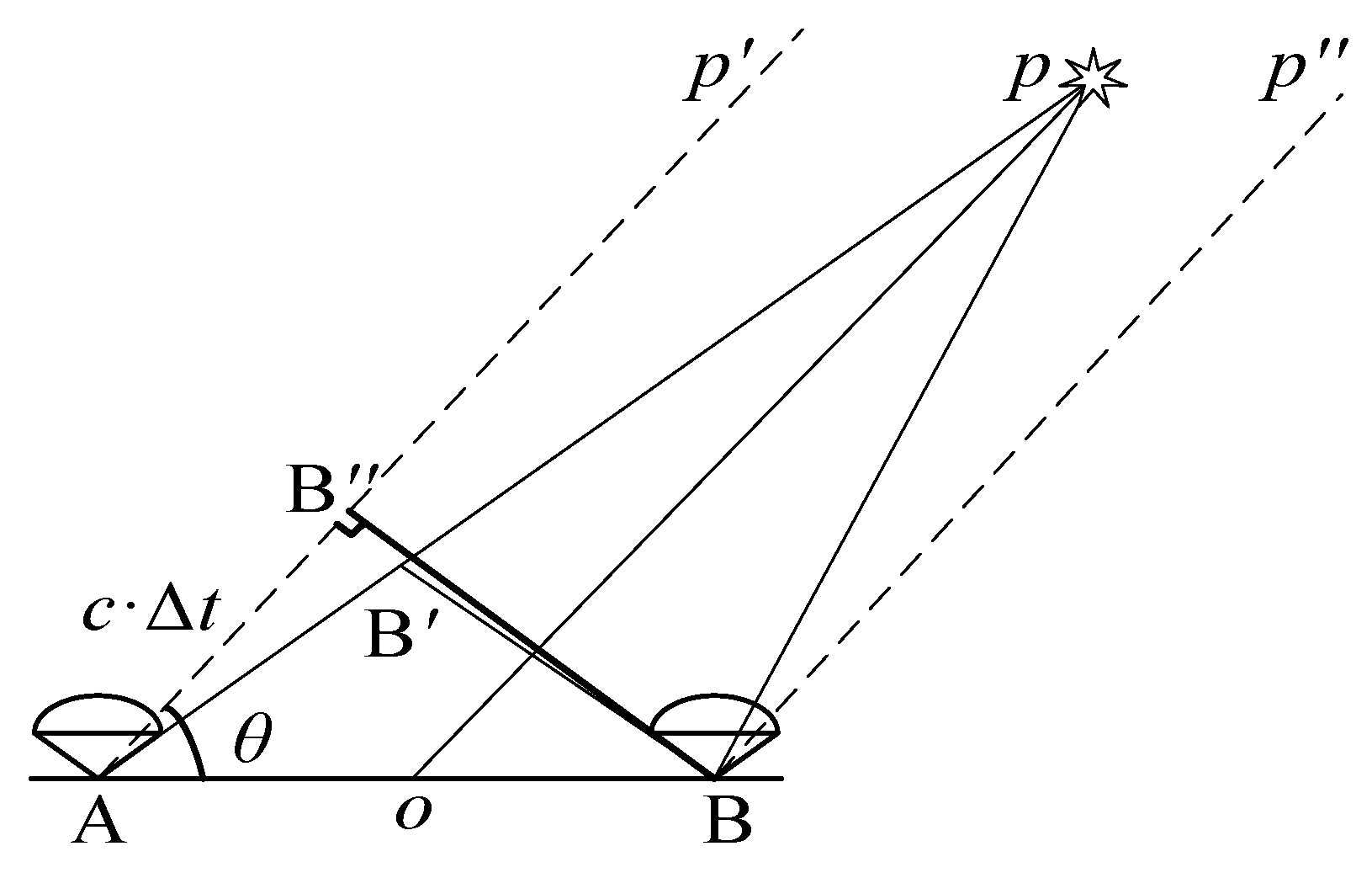
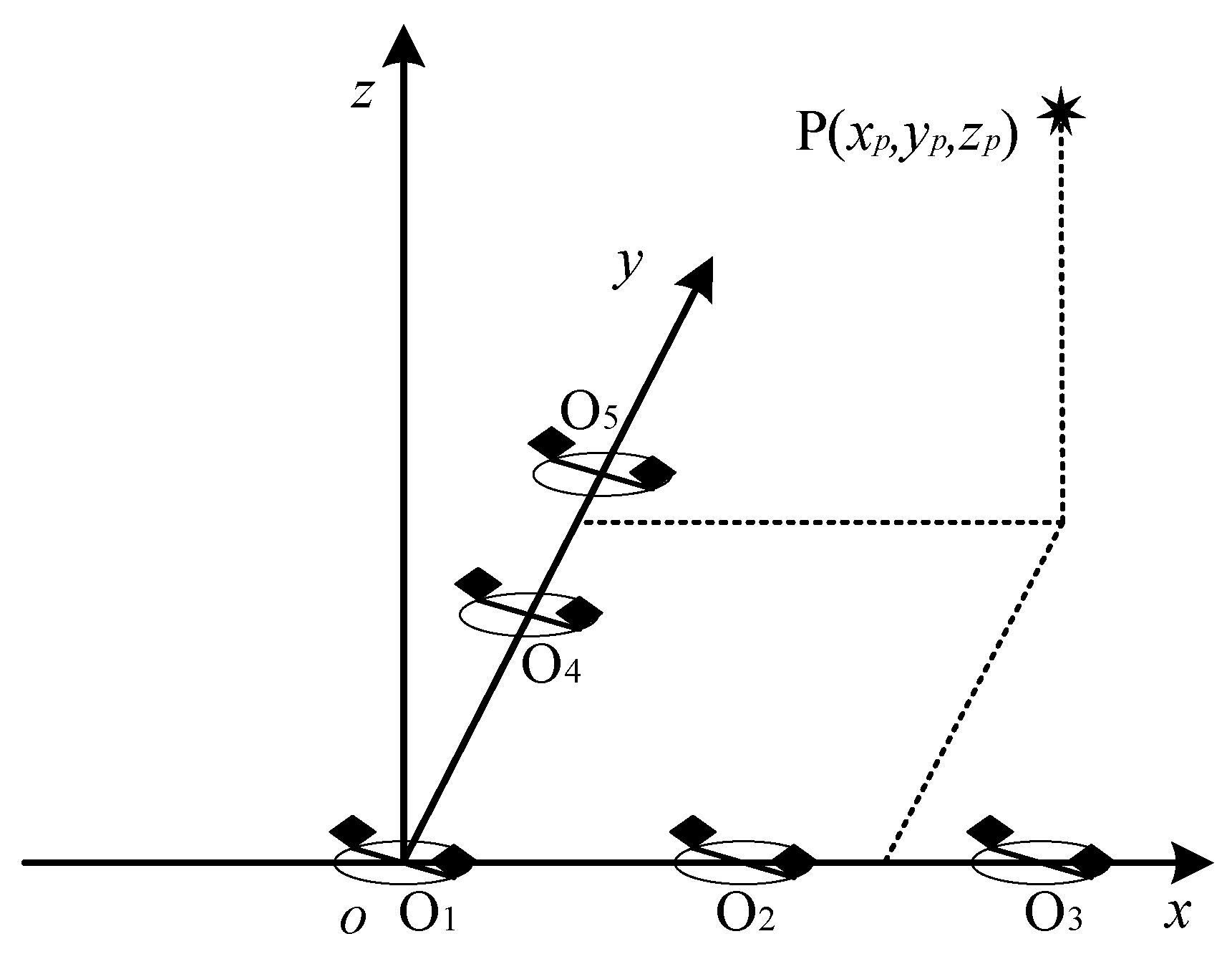
2.1. The Principle of PD Localization Based on a Symmetrical Antenna Array

When performing PD localization in a substation, the entire substation is treated as an infinite half-space. The localization principle is shown in Figure 1. Point O is the measurement point, which coincides with the coordinate origin o. In the figure, the antennas A and B are installed symmetrically at both ends of the connecting rod that rotates around the point O, and the connecting rod AB is free to rotate around the point O in the plane xoy. αj is the current rotation angle, where j is the serial number of rotation angles. θ and φ are the azimuth angle and pitch angle between the PD source and point O. Given that P is located at any point (xp, yp, zp) in space, the UHF signal radiated by the PD propagates to the directional antennas A and B via paths PA and PB. Because the lengths of the paths PA and PB are different, there is a time difference Δtj between the time (denoted as tA and tB respectively) of the two antennas receiving signals. By rotating the connecting rod, a series of time differences Δtj are obtained at different rotation angles, the time differences meet the geometric requirements demonstrated in Equation (1), where djA and djB are the distances from the PD source P to the antennas A and B, respectively, and c is the propagation speed of electromagnetic waves in the air. Based on the spatial geometric relationship, the wave path difference is demonstrated as Equation (2).
d j A d j B = c Δ t j
c Δ t j = ( x p r cos α j ) 2 + ( y p + r sin α j ) 2 + z p 2 ( x p + r cos α j ) 2 + ( y p r sin α j ) 2 + z p 2
To obtain the position of P(xp, yp, zp), at least three equations need to be solved simultaneously. Therefore, by rotating the antenna array at one detection point, two channels of UHF signals are obtained under three different αj. Next, the time delay estimation algorithm is used to calculate Δtj, and three equations are established to solve simultaneously, as shown in Equation (3), which is nonlinear and non-symmetrical.
{ d 1 A d 1 B = c Δ t 1 d 2 A d 2 B = c Δ t 2 d 3 A d 3 B = c Δ t 3

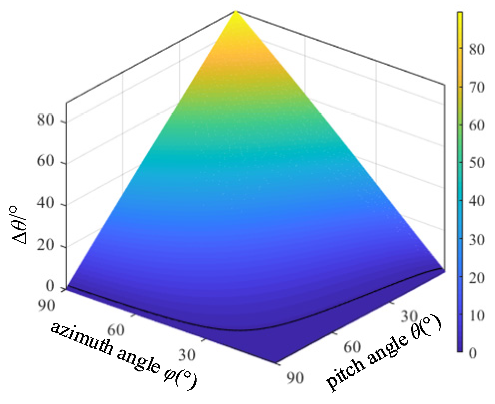
2.2. Localization Error Analysis

Theoretically, the three-dimensional coordinates of the PD source can be acquired by solving Equation (3). However, there must be time delay errors, antenna array size errors and rotation angle errors in engineering applications. There are two kinds of time delay errors. The first is a random error, which is caused by the time delay estimation algorithm caused by noise, which is caused by the low signal-to-noise ratio of the signal. The second is systematic error, which is caused by discrete sampling. The former can be reduced by increasing the signal-to-noise ratio or improving time delay estimation algorithm performance, while the latter is inevitable. The antenna array size error comes from the installation and size measurement process, which is generally small. The rotation angle error comes from the accuracy level of the angle measuring device itself. The mathematical model of the PD location is to calculate the coordinates of PD source according to the spatial geometric relationship, which is a precise process. When there are errors in the above parameters, it will cause the deviation of the spatial geometric relationship, resulting in no solution to the equations, and it is impossible to obtain the coordinates of the PD source. Therefore, iterative and optimization methods are usually used to solve the equations. However, usually only the direction angle or two-dimensional plane coordinates of the PD source can be obtained.
According to the analysis of literature [26], the PD localization method based on the TDOA algorithm can obtain a relatively accurate two-dimensional azimuth angle. However, there are still errors, and the error distribution is related to the relative position between the PD source and the antenna array. Therefore, detection is often performed at multiple detection points. The azimuth angle is obtained and then positioned on a two-dimensional plane through the intersection of the azimuth angles [27]. The principle of two-dimensional plane azimuth measurement is shown in Figure 2. A and B are the antennas at both ends of the antenna array, and the distance is 2r. p is the PD source. pA and pB denote the propagation paths of electromagnetic waves. ∆pBB′ represents the isosceles triangle. The time delay c·Δt = dAB′ of the signals is received by the two antennas A and B. When the PD source is far away from the antenna array, the propagation paths pA and pB of the UHF signal can be approximated as parallel lines, i.e., p′A//p′′B. As shown in the figure, B′′ is the vertical foot of point B on the straight line p′A, and the path distance difference c·Δt = AB′ can be approximated as c·Δt ≈ AB′′. The apparent azimuth angle θapp can be calculated by the Formula (4).
θ app = arccos c Δ t 2 r
The calculation method of the PD source azimuth obtained from Equation (4) is based on two assumptions: (1) the PD source and the antenna array are in the same plane; (2) the distance between the PD source and the antenna array is op >> 2r. Therefore, a certain error Δθ between the θapp calculated by the formula (4) and the θ in Figure 1 is inevitable. This error is illustrated by Equation (5). Figure 3 lists the error distribution with φ and θ when r = 0.75 m and z = 7.5 m. The maximum value of Δθ is 90°, which occurs at θ = 0° and φ = 90°. At the same time, there are two cases where the azimuth error is 0. The first case is when φ = 0°, no matter how many degrees θ is, the error is 0°. The physical meaning is when the height of the PD source is the same as the height of the antenna array, there is no error in the azimuth angle obtained by the simplified localization method. However, when conducting detections in the AIS, the height of the power equipment must be higher than the height of the antenna array. This situation does not exist in practice. The second case is when θ = 90°, no matter how many degrees φ is, the error is 0°. The physical outcome is that, when the projection of the PD source on the two-dimensional plane is located on the mid-perpendicular line of the antenna array, the height change of the PD source does not have any effect on the localization result. In this case, the corresponding delay is 0. Moreover, the closer θ is to 90°, the smaller the corresponding error is. Furthermore as θ deviates from the 90° direction, the height has a greater impact on the localization result.
Δ θ = θ app - θ = arccos c Δ t 2 r θ

3. An Improved PSO Algorithm-Based 3D Localization

To improve the localization accuracy, multiple detection points are selected to detect PD signals. Multiple groups of array UHF signals at different rotation angles are obtained at each measuring point. In addition, the time delay is calculated and an implicit formal equation system with redundant equations is established. This is shown in Formula (6), where k is the number of localization equations obtained at all measuring points. Based on the error analysis, by adjusting the angle of the antenna array, when the projection of the PD source on the plane is closer to the vertical line of the antenna array, the two-dimensional azimuth can be obtained more accurately. According to this conclusion, the three-dimensional localization method based on the PSO algorithm consists of two steps: the optimization of the two-dimensional plane coordinates (x, y) and the optimization of the height z. The overall process consists of five steps as follows:
Step 1: Establish the location equation system. Specifically, the PD signals at multiple rotation angles of each detection point are detected, and then the time difference is obtained using the delay estimation method. The coordinates of the detection point Om(xm, ym), the rotation angle αmn and the time delay Δtmn are recorded, where m is the number of the measurement point, n is the number of the rotation angle, and K = m n . Thus, the equation system shown in (6) is established.
{ f 1 = d 1 A d 1 B c Δ t 1 f 2 = d 2 A d 2 B c Δ t 2                                                                     f k = d k A d k B c Δ t k                                                                     f K = d K A d K B c Δ t K
Step 2: Establish a two-dimensional plane coordinate optimization objective function SP. As shown in Equation (7), where ak is the selected coefficient of the objective function and bk is the weight coefficient of the objective function. The calculation of ak is illustrated in Equation (8), where ε is the set delay threshold. In addition, bk is calculated in Equation (9).
S P = min k = 1 K a k b k f k
a k = { 1 i f       Δ t k < ε 0         e l s e
b k = 1 c Δ t k 2 L
Step 3: Locating the PD source in the two-dimensional plane based on the PSO algorithm. The coordinates (x, y) of the PD source are set as the value of the particle, and set z = 0 in Equation (6). Then, the PSO algorithm is used, and the calculation is performed based on the following four sub-steps:
(3.1) Set the number of particles i, and randomly initialize the coordinates gi(0), and other parameters, such as the number of iterations q and the speed Vi(0), where the superscript (0) indicates that the number of iterations is the 0th. In gi(0), the coordinates of the PD source in the two-dimensional plane is (xi(0), yi(0));
(3.2) Substitute the value gi(0) of the initialized particle into Equation (6) and set the ordinate z = 0 to calculate fki(0). Use Equation (6) to calculate the objective function SPi corresponding to each particle. Record the value of each particle and store it in the array gid(0), and store the particle value corresponding to the minimum value in the objective function SPi into the variable ggd(0);
(3.3) Update the spatial coordinates and velocity of each particle according to Equations (10) and (11), where w is the inertia weight, Vid(q) is the update velocity of the qth particle iteration, η1 and η2 are the acceleration constants, and rand() is a random constant between (−1~1).
V i d ( q + 1 ) = w V i d ( q ) + η 1 rand ( ) [ g i ( q ) g g d ( q ) ] + η 2 rand ( ) [ g i ( q ) g i d ( q ) ]
g i ( q + 1 ) = g i ( q ) + V i d ( q )
(3.4) Repeat steps (3.2) and (3.3) until the number of iterations is satisfied, and output the coordinates (xgd, ygd) of ggd(Q), which are the coordinates of the PD source in the two-dimensional plane.
Step 4: Establish a three-dimensional plane coordinate optimization objective function ST, and the expression form is the same as that of Equation (6). The weight coefficient bk is all 1. In order to distinguish from the ak in step 2, the selected coefficient here is expressed as ak, As shown in Equation (12).
a k = { 0 i f       Δ t k < ε 1         e l s e
Step 5: Location in three-dimensional space based on the PSO algorithm. The three-dimensional coordinates (x, y, z) of the PD source are used as the value of the particle, while the values of x and y in each particle are limited to a certain range, and this range is denoted by δ, i.e., during particle initialization and iteration, each time the assignment should be within the range of [xgdδ, xgd + δ] and [ygdδ, ygd + δ]. Then, the particle swarm optimization algorithm should be used for optimization. Calculate according to steps (3.1)–(3.4), and the optimal solution will be the output after satisfying the conditions; that is, the coordinates of the PD source in three-dimensional space.
According to the method above, the locating equations are classified based on the error distribution characteristics. In the plane coordinate solution stage, only the equations with the greatest weight of the plane coordinates are selected to be solved to ensure the accuracy of the plane coordinates. This minimizes the plane positioning error caused by assuming “op >> 2r”. In the space coordinate solution stage, the obtained plane coordinates are used to constrain the optimization range of the PSO algorithm, which effectively avoids the algorithm falling into the local optimal solution. Further, the equations that are not sensitive to height are excluded, while the locating equations that are more sensitive to height are retained, which effectively improves the accuracy of the localization results.

4. Experimental Verification
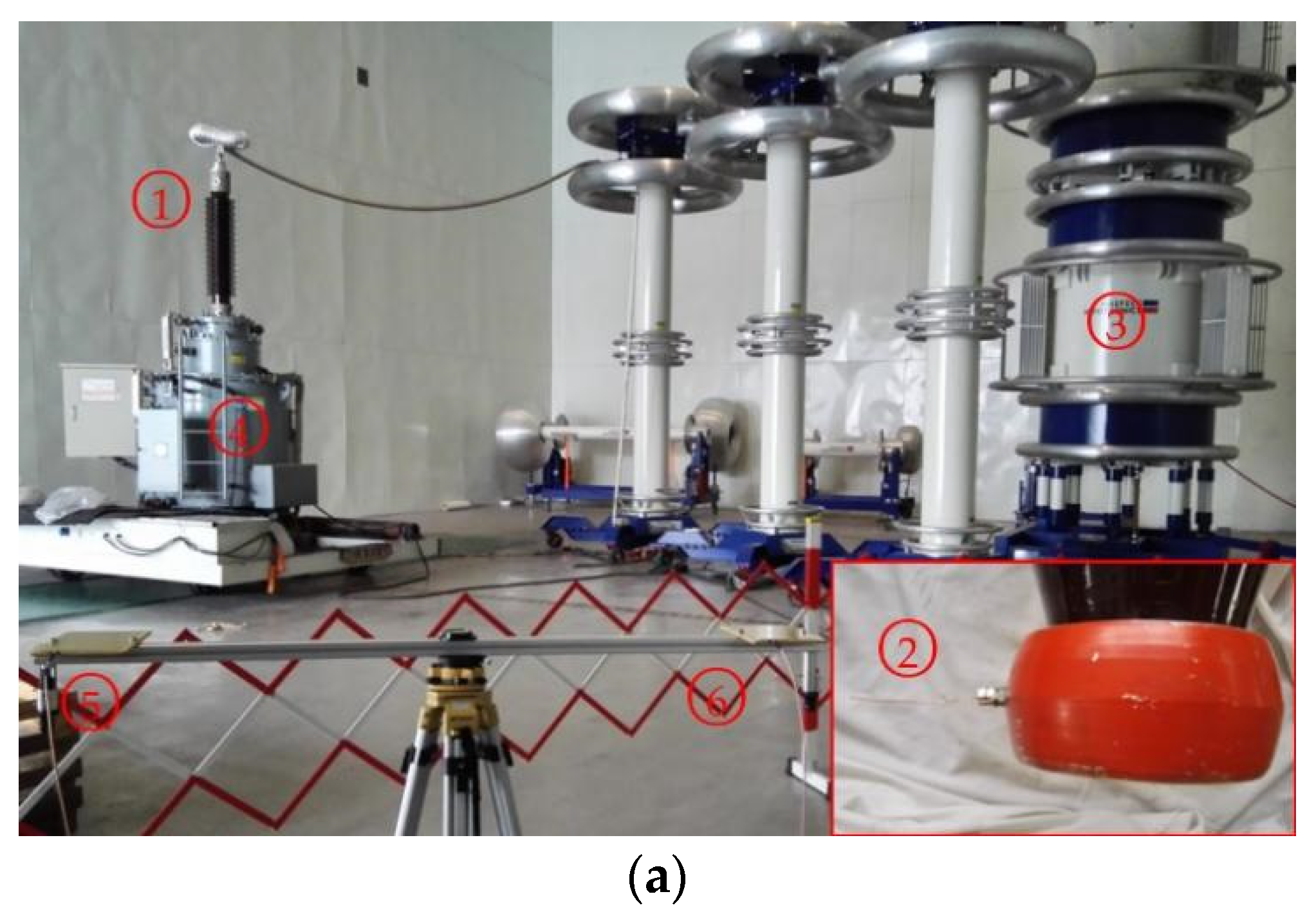
4.1. Experiment

In order to verify the proposed method, the experiment of the simulated PD source is carried out in the laboratory, and the photo of the experimental site is shown in Figure 4a. The antenna adopts the Vivaldi antenna [28] with high gain and directivity, the bandwidth is 0.5–3 GHz, and the maximum gain is 7.9 dBi. The LeCry640 oscillograph is used as the signal acquisition device, and the dual-channel sampling rate is 40 GS/s. The dividing disk is used to measure the rotation angle and take the counterclockwise rotation as the positive direction. The two antennas are connected to the testing equipment through coaxial high-frequency cables of the same model and length. The prefabricated fault 110 kV bushing is used as the detection target, and the prefabricated fault type is tip discharge in oil, as shown in the lower right corner of Figure 4. The tip electrode is installed on the equalizing ring of the bushing, and then the electrode is immersed in the transformer oil with the equalizing ring. The electric field at the tip electrode is distorted, which is the PD source. The test voltage is 74.6 kV, and the TWPD-2B multi-channel partial discharge tester is used to measure the PD in real time. The obtained PRPD map is shown in Figure 4b. The magnitude of the PD source is 95.57 PC, which can be determined as a partial discharge of insulation fault from the PRPD map.
A coordinate system is established in the laboratory. As shown in Figure 5, the height of the antenna is taken as the xoy plane, and five measuring points are selected for detection, where O1(0, 0, 0), O2(4.2, 0, 0), O3(8, 0, 0), O4(0, 3.2, 0), O5(0, 6, 0) (unit: m). Because the simulated PD source is located in the hoist seat, the UHF signal overflows from the connection between the casing and the hoist seat. The diameter of the casing flange is 0.4 m. In the coordinate system, the coordinate of the casing center is (6.5, 5.5) (unit: m), and the height of the flange is 3.47 m. Therefore, the coordinate range of the PD source is p (6.5 ± 0.2, 5.5 ± 0.2, 3.47) (unit: m). Multiple rotation angles are measured at each measuring point and six groups of UHF signals are measured for each rotation angle.

4.2. Testing Results

The UHF signal of the array when the rotation angle of the measuring point O2 is 0° is shown in Figure 6. According to the time delay estimation method provided in the literature [29], the time delay of the two signals is estimated. The time difference is −1.650 ns. The time delays obtained by the five measuring points at different rotation angles are listed in Table 1.

4.3. Data Analysis

4.3.1. Position Analysis

Based on the localization method of the third part, a set of locating equations with 30 equations is established. Firstly, the localization of the PD source in the two-dimensional plane is carried out, and further, the optimization objective function Sp in the two-dimensional plane is constructed. The expression is shown in Equation (7), where K = 30. The selection coefficient ak and the weighting coefficient bk are calculated according to Equations (8) and (9), as shown in Figure 7, where ε = 1 is set. A total of 10 equations are selected of plane coordinates, the number of particles is 500, the number of iterations is 2000, the dimension of each particle is 2, and z = 0. After calculation, the obtained plane coordinates are (6.34, 5.49) (unit: m).
Next, according to steps 4 and 5, the optimization of the three-dimensional space is conducted. The optimization objective function Sp in the three-dimensional space is constructed, shown in Equation (7). According to step 4, the selection coefficient ak and the weighting coefficient bk are reset. The number of particles is set to 500, the number of iterations is 2000, the dimension of each particle is 3, and the updated range of the plane coordinates is limited to δ = 0.4. After calculation, the obtained localization result is (6.4, 5.37, 3.31) (unit: m), where the abscissa and ordinate are within the range of the PD source p(6.5 ± 0.2, 5.5 ± 0.2, 3.47) (unit: m), and the height deviation is 0.16 m.
Combined with the size of the high-voltage equipment, this error range can effectively locate the equipment where PD occurs and the location of signal overflow.

4.3.2. Analysis of Factors

In the analysis, the parameter ε is set by the authors. To study the influence of this parameter on the localization results, different values are set for recalculation. Setting ε = 0.3, 0.7, 1, 1.3, 1.7, 2, 2.3, respectively, the calculation results are shown in Table 2. The deviation range of the results is all less than 0.6 m, and the errors are mainly concentrated in the height. This result is consistent with the error analysis results of the literature [26]. As ε varies, the error is the smallest when the number of equations selected for plane locating is 14. When the number of equations is less than or equal to 7, or greater than or equal to 18, the deviation of the plane coordinates is slightly larger. Compared with the size of the electrical equipment in the substation, the error can basically locate the equipment where PD occurs. The analysis results show that the selection of the delay threshold has a certain influence on the localization results. However, the influence is limited; thus, relatively accurate results can be obtained in practical engineering.

4.3.3. Comparison Analysis

In order to further prove the effectiveness of the method proposed in this paper, it is compared with the four localization algorithms published before. The analysis is realized from the two aspects, accuracy and efficiency. The four comparison methods are the direct particle swarm solution algorithm [25], grid search algorithm [23,24], iterative solution algorithm [30], and localization algorithm based on error probability distribution [26]. The details of various methods are shown in Table 3. The computer configuration is set as follows: an Intel Core i5-4460 system with 3.2 GHz of clock speed, 8 GB of RAM, and a 64-bit Windows 7 operating system. The localization results and time taken for the four methods are shown in Table 4.
According to the results in Table 4, the accuracy of the localization is analyzed first. There is a big difference between the four results of method A. It is a well-known problem of PSO algorithm that it can easily fall into a locally optimal solution. According to the conclusion of Section 2.2, when the rotation angle is different, the influence weight of height on time delay is different. The PSO algorithm is used to locate PD source in 3D without classifying the localization equations, and the result is that the free variation range of the third dimension of the particle is too large. Therefore, there are many locallly optimal solutions in the space, resulting in poor consistency of the results of multiple calculations. Because it is easy to fall into the local optimal solution, the deviation from the results of multiple calculations is large. Method B can only select the nodes in the grid, and due to the limitation of the grid size, it can only obtain relatively accurate coordinates in the two-dimensional plane, and the height error is large. The reason is that the height is more sensitive to the influence of the delay estimation error [26]; a small delay deviation could lead to a large height deviation. In addition, the coordinates of the grid nodes cannot be selected continuously; thus, the height error is large. Method C shows the same disadvantage. Because the height is greatly affected by the delay estimation error, there is a large error in the height in the iterative result. The calculation results of the localization method based on the method D are basically consistent with the accuracy of the method proposed in this paper. From the analysis of algorithm efficiency, Method A for 3D location has the highest efficiency, while method B requires too much computation. When the grid size is 0.25 m, the time consumption reaches 4399.88 s, and the efficiency is the lowest. Method C mainly costs too much time in the iterative stage, and the efficiency is low. Method D needs to perform the particle swarm optimization algorithm six times, and then calculate the error probability of each point in the space near the 6th azimuth angle, which reduces the efficiency. Compared with method D, the proposed method improves the efficiency by 16.13 times while ensuring the localization accuracy.

5. Conclusions

In order to improve the accuracy and efficiency of PD localization in AIS, the principle and error distribution characteristics of PD localization based on antenna arrays are analyzed in this paper, and a method based on improved PSO algorithm is proposed. The test was carried out in the laboratory to verify the method and compare with the four reported methods. Several conclusions are summarized as follows:
(1) the error distribution of the localization results is greatly affected by the relative position relationship between the PD source and the antenna array. When the projection of the PD source on the plane is located on the mid-perpendicular line of the antenna array, the azimuth error is the smallest.
(2) The locating equations are classified based on the error distribution characteristics. When calculating the plane coordinate, only the equations with the greatest weight of the plane coordinates are selected. When calculating the space coordinate, the obtained plane coordinates are used to constrain the optimization range of the PSO algorithm. The equations that are not sensitive to height are excluded. The test results show that the minimum error is 0.21 m, and the maximum error is 0.54 m. The faulty equipment can be accurately located with this error.
(3) Comparing with the four reported methods in both accuracy and efficiency with the same locating equations, the accuracy of the proposed method is consistent with the existing high-accuracy method; however, the efficiency is increased by 16.13 times.
The use of the proposed method can greatly improve both efficiency and accuracy, which is more suitable for applications in AIS. However, the structure of the equipment needs to be reformed to make it suitable for convenient movement in AIS. At the same time, it needs to be tested and applied repeatedly in AIS to further improve the performance of the equipment and algorithm. Of course, this is an urgent problem to be studied in the next steps.

Author Contributions

P.L. contributed to the conception of the study, the background research, method design and analysis of the experimental results; X.P. wrote the manuscript; K.Y. provided methodological guidance, writing review and funding support; Y.X. reviewed and revised the manuscript; R.W. performed methodological guidance and writing review. Z.M. carried out the experiment. All authors have read and agreed to the published version of the manuscript.

Funding

This research is funded by the Project of the Science and Technology Department of Henan Province under Grant 212102210017 and 222102220116.

Institutional Review Board Statement

Not applicable.

Informed Consent Statement

Not applicable.

Data Availability Statement

Not applicable.

Conflicts of Interest

The authors declare no conflict of interest.

References

  1. Abdel-Gawad, N.M.; El Dein, A.Z.; Mansour DE, A.; Ahmed, H.M.; Darwish, M.M.; Lehtonen, M. PVC nanocomposites for cable insulation with enhanced dielectric properties, partial discharge resistance and mechanical performance. High Volt. 2020, 5, 463–471. [Google Scholar] [CrossRef]
  2. Abdel-Gawad, N.M.; El Dein, A.Z.; Mansour DE, A.; Ahmed, H.M.; Darwish MM, F.; Lehtonen, M. Experimental measurements of partial discharge activity within LDPE/TiO2 nanocomposites. In Proceedings of the 2017 Nineteenth International Middle East Power Systems Conference (MEPCON), Cairo, Egypt, 19–21 December 2017; pp. 811–816. [Google Scholar]
  3. Abdel-Gawad, N.M.; Mansour DE, A.; Darwish MM, F.; El Dein, A.Z.; Ahmed, H.M.; Lehtonen, M. Impact of nanoparticles functionalization on partial discharge activity within PVC/SiO2 nanocomposites. In Proceedings of the 2018 IEEE 2nd International Conference on Dielectrics (ICD), Budapest, Hungary, 1–5 July 2018; pp. 1–4. [Google Scholar]
  4. Cheng, J.; Xu, Y.; Ding, D.; Liu, W. Investigation of the UHF Partial Discharge Detection Characteristics of a Novel Bushing Tap Sensor for Transformers. IEEE Trans. Power Deliv. 2020, 36, 2748–2757. [Google Scholar] [CrossRef]
  5. Zhou, L.; Cai, J.; Hu, J.; Lang, G.; Guo, L.; Wei, L. A Correction-iteration Method for Partial Discharge Localization in Transformer based on Acoustic Measurement. IEEE Trans. Power Deliv. 2020, 36, 1571–1581. [Google Scholar] [CrossRef]
  6. Zhang, X.; Shi, M.; He, C.; Li, J. On Site Oscillating Lightning Impulse Test and Insulation Diagnose for Power Transformers. IEEE Trans. Power Deliv. 2020, 35, 2548–2550. [Google Scholar] [CrossRef]
  7. Ning, S.; He, Y.; Yuan, L.; Sui, Y.; Huang, Y.; Cheng, T. A Novel Localization Method of Partial Discharge Sources in Substations Based on UHF Antenna and TSVD Regularization. IEEE Sens. J. 2021, 21, 17040–17052. [Google Scholar] [CrossRef]
  8. Zhu, M.; Wang, Y.; Liu, Q.; Zhang, J.; Deng, J.; Zhang, G.; Shao, X.; He, W. Localization of multiple partial discharge sources in air-insulated substation using probability-based algorithm. IEEE Trans. Dielectr. Electr. Insul. 2017, 24, 157–166. [Google Scholar] [CrossRef]
  9. Li, Z.; Luo, L.; Zhou, N.; Sheng, G.; Jiang, X. A Novel Partial Discharge Localization Method in Substation Based on a Wireless UHF Sensor Array. Sensors 2017, 17, 1909. [Google Scholar] [CrossRef]
  10. Dhara, S.; Koley, C.; Chakravorti, S. A UHF Sensor Based Partial Discharge Monitoring System for Air Insulated Electrical Substations. IEEE Trans. Power Deliv. 2020, 36, 3649–3656. [Google Scholar] [CrossRef]
  11. Hou, H.; Sheng, G.; Jiang, X. Robust Time Delay Estimation Method for Locating UHF Signals of Partial Discharge in Substation. IEEE Trans. Power Deliv. 2013, 28, 1960–1968. [Google Scholar]
  12. Sinaga, H.H.; Phung, B.T.; Blackburn, T.R. Partial discharge localization in transformers using UHF detection method. IEEE Trans. Dielectr. Electr. Insul. 2012, 19, 1891–1990. [Google Scholar] [CrossRef]
  13. Judd, M.D.; Farish, O.; Hampton, B.F. The excitation of UHF signals by partial discharges in GIS. IEEE Trans. Dielectr. Electr. Insul. 1996, 3, 213–228. [Google Scholar] [CrossRef]
  14. Portugues, I.E.; Moore, P.J.; Glover, I.A.; Johnstone, C.; McKosky, R.H.; Goff, M.B.; van der Zel, L. RF-Based Partial Discharge Early Warning System for Air-Insulated Substations. IEEE Trans. Power Deliv. 2009, 24, 20–29. [Google Scholar] [CrossRef]
  15. He, J.; Li, M.; Chen, G.; Wang, Z. Error analysis and antenna array placement optimization of localization system for partial discharge in substation. Prz. Elektrotechniczny 2014, 90, 104–107. [Google Scholar]
  16. Wenjun, Z.; Pengfei, L.; Shuai, Y.; Yushun, L.; Yan, T.; Yong, W. Partial Discharge Localization Method by Multi-direction Measurement Using Directional Antenna in Substation. Gaodianya Jishu/High Volt. Eng. 2017, 43, 1476–1484. [Google Scholar]
  17. Xavier, G.V.; de Oliveira, A.C.; Silva, A.D.; Nobrega, L.A.; da Costa, E.G.; Serres, A.J. Application of Time Difference of Arrival Methods in the Localization of Partial Discharge Sources Detected Using Bio-Inspired UHF Sensors. IEEE Sens. J. 2020, 21, 1947–1956. [Google Scholar] [CrossRef]
  18. Wang, S.; He, Y.; Yin, B.; Ning, S.; Zeng, W. Partial Discharge Localization in Substations Using a Regularization Method. IEEE Trans. Power Deliv. 2020, 6, 822–830. [Google Scholar] [CrossRef]
  19. Zhu, M.X.; Wang, Y.B.; Liu, Q.; Zhang, J.N.; Deng, J.B.; Zhang, G.J.; Shao, X.J.; He, W.L. Localization of Partial Discharge Signals Based on Ultra-high-frequency Antenna Array and Analysis of Influence Factors. High Volt. Appar. 2019, 55, 53–60. [Google Scholar]
  20. Khan, U.F.; Lazaridis, P.I.; Mohamed, H.; Albarracín, R.; Zaharis, Z.D.; Atkinson, R.C.; Tachtatzis, C.; Glover, I.A. An Efficient Algorithm for Partial Discharge Localization in High-Voltage Systems Using Received Signal Strength. Sensors 2018, 18, 4000. [Google Scholar] [CrossRef] [Green Version]
  21. Zheng, Q.; Luo, L.; Song, H.; Sheng, G.; Jiang, X. Fault Early Warning in Air-insulated Substations by RSSI-Based Angle of Arrival Estimation and Monopole UHF Wireless Sensor Array. IET Gener. Transm. Distrib. 2020, 14, 2345–2361. [Google Scholar]
  22. Zheng, Q.; Luo, L.; Song, H.; Sheng, G.; Jiang, X. A RSSI-AOA Based UHF Partial Discharge Localization Method Using MUSIC Algorithm. IEEE Trans. Instrum. Meas. 2021, 70, 1–9. [Google Scholar] [CrossRef]
  23. Wei, B.; Yu, G.F.; Liu, F.; Sun, H.J.; Li, H.J. Research on Location Method of PD Signal for Metal-Clad Switchgear. Appl. Mech. Mater. 2017, 864, 231–236. [Google Scholar] [CrossRef]
  24. Hou, H.; Sheng, G.H.; Miao, P.Q.; Li, X.W.; Hu, Y.; Jiang, X.C. Partial Discharge Location Based on Radio Frequency Antenna Array in Substation. High Volt. Eng. 2012, 38, 1334–1340. [Google Scholar]
  25. Wang, S.; He, Y.; Yin, B.; Zeng, W.; Li, C.; Ning, S. Multi-Resolution Generalized S-Transform Denoising for Precise Localization of Partial Discharge in Substations. IEEE Sens. J. 2020, 21, 4966–4980. [Google Scholar] [CrossRef]
  26. Li, P.; Zhou, W.; Yang, S.; Liu, Y.; Tian, Y.; Wang, Y. A Novel Method for Partial Discharge Localization in Air-insulated Substations. IET Sci. Meas. Technol. 2017, 11, 331–338. [Google Scholar] [CrossRef]
  27. Hou, H.; Sheng, G.; Jiang, X. Localization Algorithm for the PD Source in Substation Based on L-Shaped Antenna Array Signal Processing. IEEE Trans. Power Deliv. 2015, 30, 472–479. [Google Scholar] [CrossRef]
  28. Liu, Y.; Zhou, W.; Yang, S.; Li, W.; Li, P.; Yang, S. A Novel Miniaturized Vivaldi Antenna Using Tapered Slot Edge with Resonant Cavity Structure for Ultra-wide Band Applications. IEEE Antennas Wirel. Propag. Lett. 2016, 15, 1881–1884. [Google Scholar] [CrossRef]
  29. Li, P.; Dai, K.; Zhang, T.; Jin, Y.; Liu, Y.; Liao, Y. An accurate and efficient time delay estimation method of ultra-high frequency signals for partial discharge localization in substations. Sensors 2018, 18, 3439. [Google Scholar] [CrossRef] [Green Version]
  30. Zheng, S.; Li, C.; He, M. A Novel Method of Newton Iteration in Complex Field and Lattice Search for Locating Partial Discharges in Transformers. Proc. CSEE 2013, 33, 155–161. [Google Scholar]
Figure 1. The principle of PD source location based on directional antenna.
Symmetry 14 01241 g001
Figure 2. The azimuth position method of PD source based on dual antenna.
Symmetry 14 01241 g002
Figure 3. The relationship of Δθ, φ and θ (r = 0.75 m, h = 7.5 m).
Symmetry 14 01241 g003
Figure 4. The laboratory testing site and the measuring result. (a)The picture of the testing site. ① the bushing with prefabricated fault, ② type of the prefabricated fault, ③ testing transformer, ④ the hoist seat, ⑤ antenna A, ⑥ antenna B. (b)The picture of phase-resolved partial discharge of the prefabricated fault.
Symmetry 14 01241 g004aSymmetry 14 01241 g004b
Figure 5. Positional relationship between PD source and detection point.
Symmetry 14 01241 g005
Figure 6. Two UHF signals of measuring point O2 with αj = 0°.
Symmetry 14 01241 g006
Figure 7. Selected coefficients and weight coefficients.
Symmetry 14 01241 g007
Table 1. Time delays obtained by the five measuring points at different rotation angles.
Testing Point (m)Rotation Angle (°)Time Delay (ns)
O1 (0, 0, 0)310−0.050
2603.500
2802.375
320−0.825
335−1.900
0−3.550
O2 (4.2, 0, 0)0−1.650
20−2.975
3380.025
3241.050
3072.250
2833.500
O3 (8, 0, 0)01.175
15−0.025
28−0.900
60−3.100
3511.700
3183.650
O4 (0, 3, 0)0−4.200
2910.025
340−3.400
300−0.650
2781.050
2423.300
O5 (0, 6, 0)2660.000
325−3.75
289−1.700
275−0.750
2600.450
2401.950
Table 2. Localization results and error analysis with different ε.
εThe Number of Selected akLocalization Results (m)Error Analysis
Whether the Plane Coordinates Are in RangeHeight Error (m)Absolute Error (Distance from Center Position) (m)
0.356.37, 5.04, 3.22N0.250.54
0.776.39, 5.08, 3.16N0.310.53
1106.4, 5.37, 3.31Y0.160.23
1.3136.38, 5.41, 3.33Y0.140.21
1.7146.36, 5.33, 3.29Y0.180.28
2186.44, 5.28, 3.11N0.360.42
2.3196.42, 5.19, 3.04N0.430.53
Table 3. Description of the Four Localization Methods.
Localization MethodsName of MethodsPrinciple DescriptionKey
Parameters
Method ADirect Particle Swarm Solution AlgorithmSimilarly to step 4 and step 5 in the algorithm described in the Section 3, the dimension of the particle is set to 3, and the objective function is the same as Equation (7), where ak and bk are all set to 1.The number of iterations and the number of particles
Method BSpatial grid search algorithmThe three-dimensional space is meshed, the grid node coordinates are brought into the equation system, and the node corresponding to the minimum deviation value is used as the position of the PD source.grid size
Method CIterative grid search solution algorithmFirst, the Newton iterative algorithm is used to solve the equation system. Secondly, the grid search algorithm is used to search around the solution result of the iterative method. Next, the node corresponding to the minimum deviation value is used as the position of the PD source.Number of iterations; Grid size; Search range
Method DError Probability Distribution- localization algorithmBased on the equations of each detection point, a system of equations is established. The particle swarm algorithm is used to calculate the azimuth and elevation angles of the PD source, to calculate the error law, to calculate the error probability of each point in the space, and to calculate the error probability of the azimuth and elevation angles of all detection points. The coordinate corresponding to the minimum value of the superimposed value is used as the position of the PD source.The number of iterations and the number of particles
Table 4. The localization results and time taken for various methods.
Localization MethodsSettings of Key ParametersLocalization Results and ErrorsTime (s)
Results (m)Absolute Error (m)
Method Anumber of iterations 2000, number of particles 500, calculate four times(0.03, 0.01, 0.01)9.1622.33
(5.67, 5.47, 2.74)1.1121.59
(6.29, 5.11, 3.64)0.4723.35
(5.84, 4.88, 3.03)1.0122.78
Method Bgrid size 0.5 m, search range 30 m × 30 m × 20 m(6.5, 5, 0.5)3.0222.05
grid size 0.25 m, search range 30 m × 30 m × 20 m(6.5, 5.25, 0.25)3.234399.88
Method Cnumber of iterations 2000, search objective ± 0.5 m(6.41, 5.01, 1.25)2.28824.36
Method Dnumber of iterations 2000, number of particles 500(6.44, 5.42, 3.32)0.18682.18
Proposed methodnumber of iterations 2000, number of particles 500(6.38, 5.41, 3.33)0.2142.29
Publisher’s Note: MDPI stays neutral with regard to jurisdictional claims in published maps and institutional affiliations.

