Article

Type II Half-Logistic Odd Fréchet Class of Distributions: Statistical Theory and Applications

by
Salem A. Alyami
1,
Moolath Girish Babu
2,†,
Ibrahim Elbatal
1,†,
Naif Alotaibi
1,† and
Mohammed Elgarhy
3,*,†
1
Department of Mathematics and Statistics, College of Science Imam Mohammad Ibn Saud Islamic University (IMSIU), Riyadh 11432, Saudi Arabia
2
Department of Statistics, CHMKM Government Arts and Science College, Kozhikode 673 572, India
3
The Higher Institute of Commercial Sciences, Al Mahalla Al Kubra 31951, Algharbia, Egypt
*
Author to whom correspondence should be addressed.
These authors contributed equally to this work.
Symmetry 2022, 14(6), 1222; https://doi.org/10.3390/sym14061222
Submission received: 13 May 2022 / Revised: 2 June 2022 / Accepted: 6 June 2022 / Published: 13 June 2022

Abstract

:
A new class of statistical distributions called the Type II half-Logistic odd Fréchet-G class is proposed. The new class is a continuation of the unusual Fréchet class. This class is analytically feasible and could be used to evaluate real-world data effectively. The new suggested class of distributions has many new symmetrical and asymmetrical sub-models. We propose new four sub-models from the new class of distributions which are called Type II half-Logistic odd Fréchet exponential distribution, Type II half-Logistic odd Fréchet Rayleigh distribution, Type II half-Logistic odd Fréchet Weibull distribution, and Type II half-Logistic odd Fréchet Lindley distribution. Some statistical features of Type II half-Logistic odd Fréchet-G class such as ordinary moments (ORMs), incomplete moments (INMs), moment generating function (MGEF), residual life (REL), and reversed residual life (RREL) functions, and Rényi entropy (RéE) are derived. Six methods of estimation such as maximum likelihood, least-square, a maximum product of spacing, weighted least square, Cramér-von Mises, and Anderson–Darling are produced to estimate the parameters. To test the six estimation methods’ performance, a simulation study is conducted. Four real-world data sets are utilized to highlight the importance and applicability of the proposed method.

1. Introduction

Today, there is a need for mathematical models required to retrieve all of the information from data and the ability to engage with it and make it usable in engineering, biological study, economics, and environmental sciences, to name a few examples. A lot of generations of academics have so far concentrated their efforts to build larger classes of distributions. The classic strategy consists of adding (parameters) to a scale or shape to the baseline model, also through the use of special functions (beta, gamma, excessive geometry, etc.), which makes the resulting distribution more adaptable, which is useful for understanding the behavior of density shapes and hazard rate shapes, for checking the goodness of fit of proposed distributions, or the flexibility on some important modeling aspects such as mean E(X), variance V(X), distribution tails, skewness (SK), kurtosis (KU), etc. Consequently, new different classes of continuous distributions have been offered, including those produced in the statistical literature listed below. Some well-known classes are the Fréchet class defined in [1], Marshall–Olkin class given in [2], beta-class given in [3], the generalized log-logistic class given in [4], the odd exponentiated half logistic (HL) class given in [5], the generalized odd log-logistic class given in [6], the Type I HL class given in [7], the logistic-X class given in [8], generalized odd log-logistic class given in [9], Kumaraswamy Type I HL class given in [10], the transmuted odd Fréchet ( O F )-class given in [11], extended O F -G class given in [12], transmuted geometric-G [13], odd Perks-G class [14], odd Lindley-G in [15], truncated Cauchy power Weibull-G [16], generalized transmuted-G [17], truncated Cauchy power-G in [18], Burr X-G (BX-G) class [19], odd inverse power generalized Weibull-G [20], Type II exponentiated half-Logistic-G in [21], Topp Leone -G in [22], exponentiated M-G by [23], odd Nadarajah–Haghighi-G in [24], exponentiated truncated inverse Weibull-G in [25], T-X generator proposed in [26], among others.
Several Fréchet classes have been judged successful in a variety of statistical applications in the last years as [27] proposed a four-parameter model named the exponential transmuted Fréchet distribution, which extends the Fréchet distribution. Ref [1] proposed the O F G class of distributions with distribution function (cdf) and density function (pdf), respectively, are follows, for x > 0
G O F r ( x ; θ ) = e G ¯ ( x , φ ) G ( x , φ ) θ ,
and
g O F r ( x ; θ ) = θ g ( x , φ ) 1 G ( x , φ ) θ 1 G ( x , φ ) θ + 1 e G ¯ ( x , φ ) G ( x , φ ) θ ,
where θ > 0 is a shape parameter, G ( x , φ ) and g ( x , φ ) are the pdf and cdf of a baseline continuous distribution with φ as parameter vector, respectively.
The O F G class was successfully considered in various statistical applications over the last few years. This reputation can be explained by its simple and versatile exponential-odd form, with the use of just one additional parameter, very different from the other current families. Ref [28] represented a new class of continuous distributions with an extra scale parameter α > 0 called the Type II HL-G ( T I I H L G ) class. The cdf and pdf of the T I I H L G class of distributions, respectively, are provided by
F ( x ) = 2 G ( x ) α 1 + [ G ( x ) ] α ,
and
f ( x ) = 2 α g ( x ) G ( x ) α 1 1 + G ( x ) α 2 .
The failure (hazard) rate function (hrf) is defined by
τ ( x ) = 2 α g ( x ) G ( x ) α 1 1 G ( x ) 2 α .
In this paper, we discuss a new extension of the odd Fréchet-G class for a given baseline distribution with cdf G ( x , φ ) using the Type II HL generator and this class is called the Type II HL odd Fréchet-G ( T I I H L O F G ) class of distributions. This new suggested class of distributions is very flexible and has many new symmetrical and asymmetrical sub-models. The cdf of ( T I I H L O F G ) class is obtained by inserting Equation (1) in Equation (3), we get
F ( x , α , θ , φ ) = 2 e α G ¯ ( x , φ ) G ( x , φ ) θ 1 + e α G ¯ ( x , φ ) G ( x , φ ) θ , x > 0 .
For each baseline G, the T I I H L O F G cdf is given by Equation (6). The corresponding pdf is
f ( x ; α , θ , φ ) = 2 α θ g ( x , φ ) G ¯ ( x , φ ) θ 1 G ( x , φ ) θ + 1 e α G ¯ ( x , φ ) G ( x , φ ) θ 1 + e α G ¯ ( x , φ ) G ( x , φ ) θ 2 .
The hrf of T I I H L O F G class is provided by
χ ( x ) = 2 α θ g ( x , φ ) G ¯ ( x , φ ) θ 1 e α G ¯ ( x , φ ) G ( x , φ ) θ G ( x , φ ) θ + 1 1 e 2 α G ¯ ( x , φ ) G ( x , φ ) θ .
The T I I H L O F G quantile function (qf) is given below
F 1 ( u ) = Q G ( u ) = G 1 1 1 + 1 α log ( u 2 u ) 1 θ .
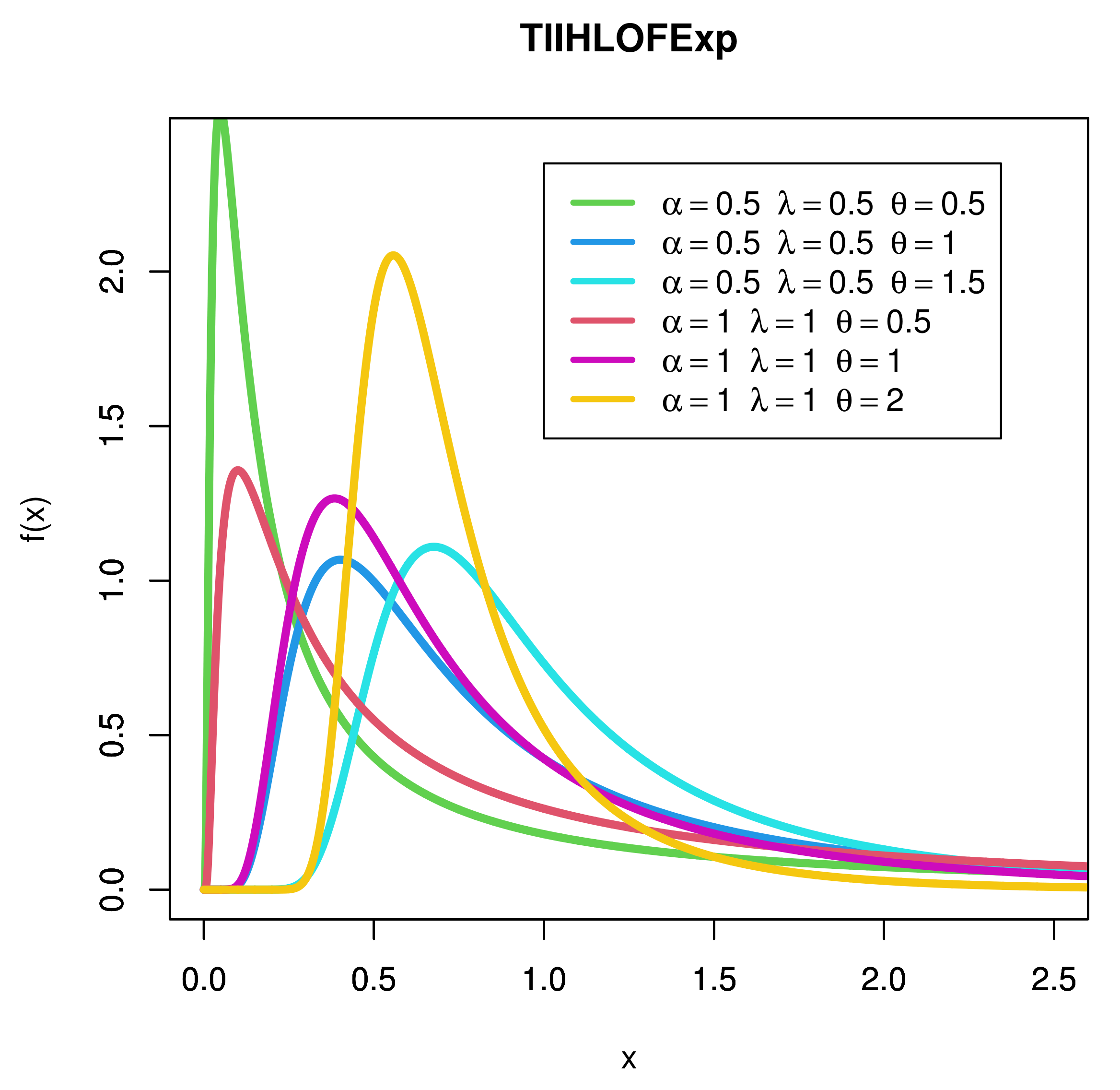
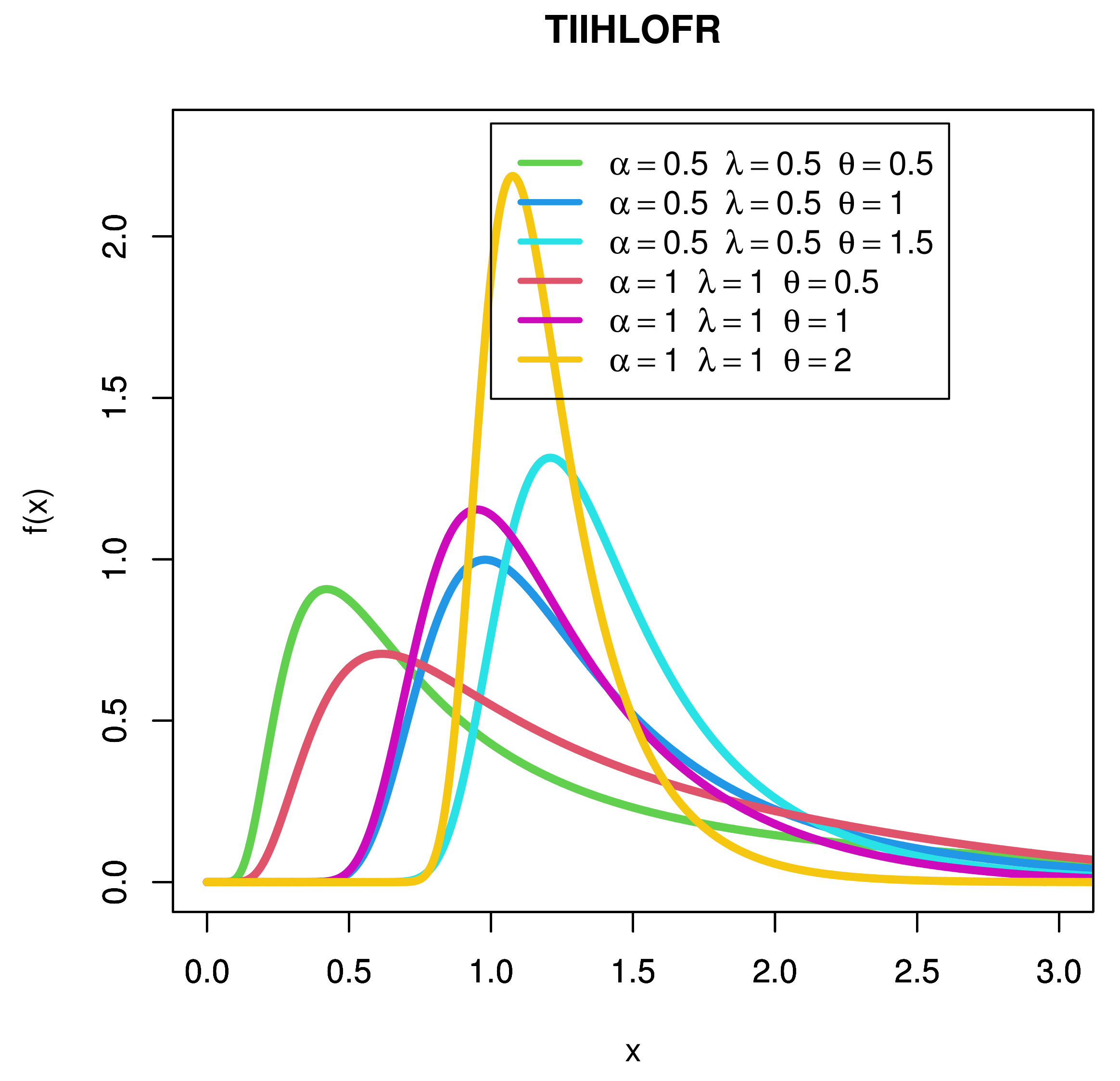
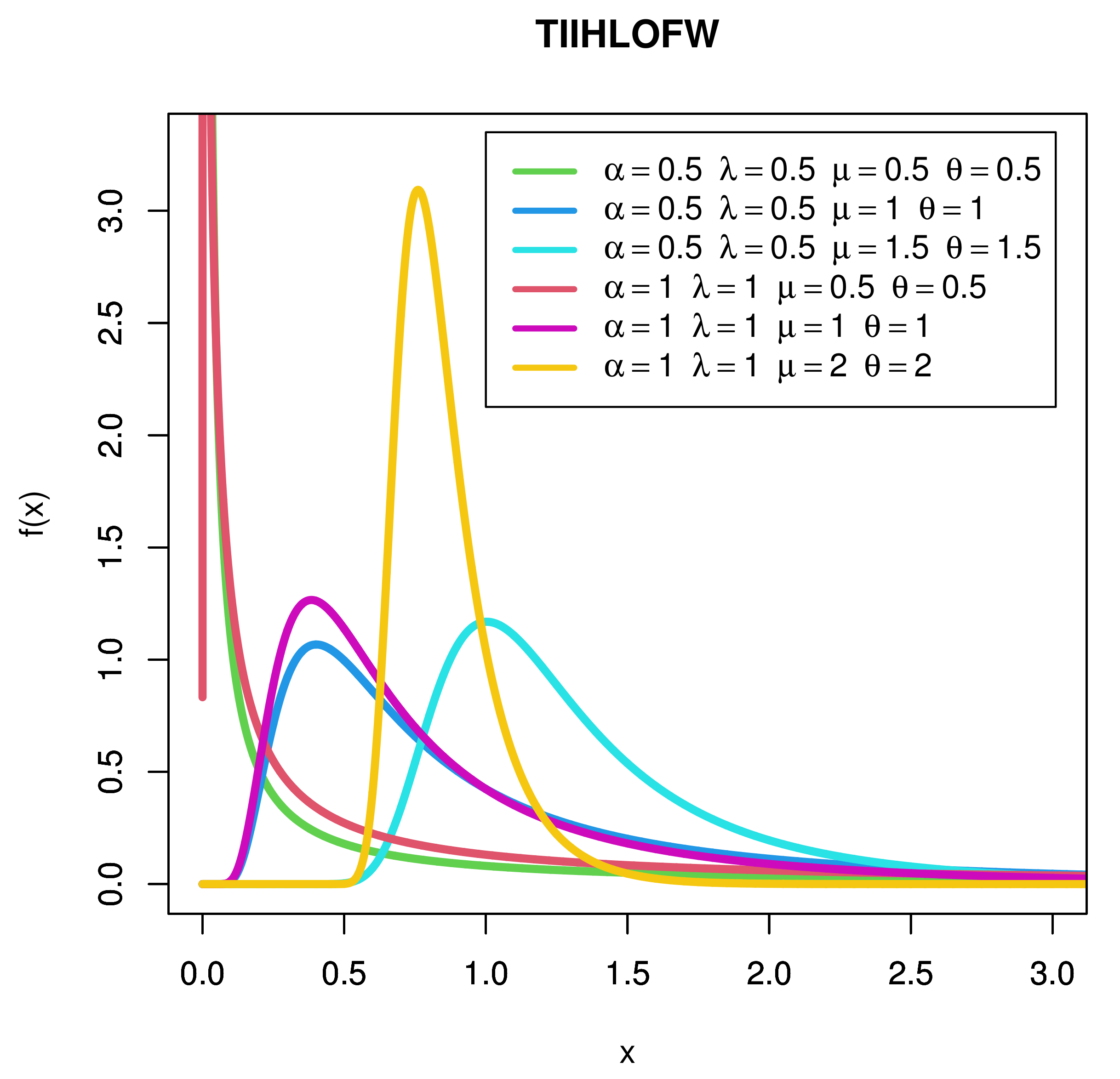
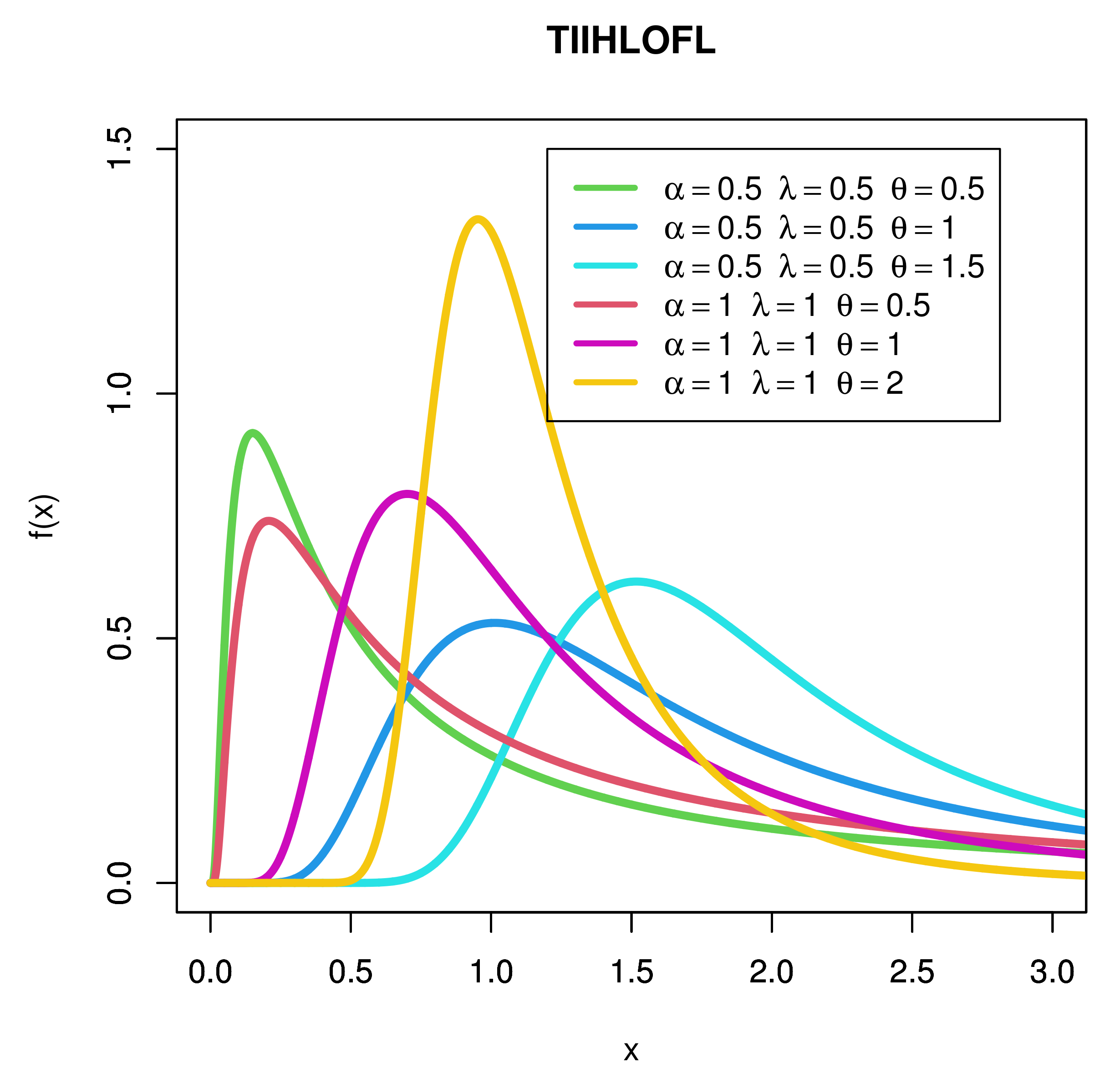
The fundamental goal of the article under consideration is to introduce a new class of statistical distributions called the Type II half-Logistic odd Fréchet-G class (TIIHLOF-G for short) as well as to investigate its statistical characteristics. The following points provide sufficient incentive to study the proposed class of distributions. We specify it as follows: (i) the new class of distributions are very flexible and have many new symmetrical and asymmetrical sub-models; (ii) it is remarkable to observe the flexibility of the proposed family with the diverse graphical shapes of probability density functions (pdf) and hazard rate functions (hrf). So, the form analysis of the corresponding pdf and hrf has shown new characteristics, revealing the unseen fitting potential of the TIIHLOF-G; (iii) the new suggested class has a closed form of the quantile function; (iv) six methods of estimation are proposed to assess the behavior of the parameters; (v) the TIIHLOF-G is very flexible and applicable. This ability of the new class is explored using four real-life data sets proving the practical utility of the model being featured.
The substance of the article is arranged as follows: Section 2 presents a linear representation of the T I I H L O F G class density. Four new sub-models are provided in Section 3. Section 4 contains a number of statistical features such as ORMs, INMs, MGEF, REL, and RREL functions, and RéE. In Section 5, different estimation methods of the model parameters are determined. Section 6 shows simulation results. Section 7 investigates three real-world data sets to demonstrate the flexibility and potential of the T I I H L O F G class using the T I I H L O F E x p and T I I H L O F W distributions. Finally, in Section 8, the conclusions are offered.

2. Useful Expansion

Assuming z < 1 and b > 0 be a real non-integer, then the next binomial expansions occur.
( 1 + z ) b = k = 0 ( 1 ) k Γ ( b + k ) k ! Γ ( b ) z k .
Applying Equation (9) to the last term in Equation (7), then
f T I I H L O F G ( x ) = 2 α θ g ( x , φ ) G ¯ ( x , φ ) θ 1 G ( x , φ ) θ + 1 i = 0 ( i + 1 ) e α ( i + 1 ) G ¯ ( x , φ ) G ( x , φ ) θ .
The exponential function’s power series now yields
e α ( i + 1 ) G ¯ ( x , φ ) G ( x , φ ) θ = j = 0 ( 1 ) j α j ( i + 1 ) j j ! G ¯ ( x , φ ) θ j G ( x , φ ) θ j .
Inserting Equation (11) in Equation (10), then
f T I I H L O F G ( x ) = g ( x , φ ) i , j = 0 2 θ ( 1 ) j α j + 1 ( i + 1 ) j + 1 j ! G ¯ ( x , φ ) θ ( j + 1 ) 1 G ( x , φ ) θ ( j + 1 ) + 1 ,
using the generalized binomial expansion to ( 1 G ( x ; φ ) ) θ ( j + 1 ) + 1 ,
( 1 G ( x ; φ ) ) θ ( j + 1 ) + 1 = k = 0 Γ ( θ ( j + 1 ) + k + 1 ) k ! Γ ( θ ( j + 1 ) + 1 ) G ( x ; φ ) k ,
and
( 1 G ( x ; φ ) ) θ ( j + 1 ) + k + 1 = d = 0 ( 1 ) d θ ( j + 1 ) + k + 1 d G ( x ; φ ) d .
The T I I H L O F pdf is an endless combination of exp-G pdfs
f T I I H L O F G ( x ) = d = 0 ϖ d h ( d + 1 ) ( x ) ,
where
ϖ d = i , j , k = 0 2 θ ( 1 ) j + d α j + 1 ( i + 1 ) j + 1 Γ ( θ ( j + 1 ) + k + 1 ) j ! k ! Γ ( θ ( j + 1 ) + 1 ) ( d + 1 ) θ ( j + 1 ) + k + 1 d ,
and h ( d + 1 ) ( x ) = ( d + 1 ) g ( x ) G d ( x ) .

3. Submodels of the TIIHLOF-G Class

We exhibit four sub-models of the T I I H L O F G distribution class.

3.1. Type II Half-Logistic Odd Fréchet Exponential (TIIHLOFExp) Distribution

Let G ( x ) and g ( x ) in Equations (6) and (7) be the cdf and pdf of Exp distribution where G ( x ; φ ) = 1 e λ x and g ( x ; φ ) = λ e λ x . The cdf and pdf of Type II half-Logistic odd Fréchet Exp ( T I I H L O F E x p ) are given below
F ( x ) = 2 e α e λ x 1 e λ x θ 1 + e α e λ x 1 e λ x θ , x > 0 ,
and
f ( x ) = 2 α θ λ e λ x ( e λ x ) θ 1 ( 1 e λ x ) θ + 1 e α e λ x 1 e λ x θ 1 + e α e λ x 1 e λ x θ 2 .
Figure 1 describes the different forms of the pdf of TIIHLOFExp distribution.

3.2. Type II Half-Logistic Odd Fréchet Rayleigh (TIIHLOFR) Distribution

Here we take G ( x ) = 1 e λ 2 x 2 and g ( x ; φ ) = λ x e λ 2 x 2 be the Rayleigh distribution. The cdf and pdf of T I I H L O F R model, are given below
F ( x ) = 2 e α e λ 2 x 2 1 e λ 2 x 2 θ 1 + e α e λ 2 x 2 1 e λ 2 x 2 θ , x > 0 ,
and
f ( x ) = 2 α θ λ x e λ 2 x 2 ( e λ 2 x 2 ) θ 1 ( 1 e λ 2 x 2 ) θ + 1 e α e λ 2 x 2 1 e λ 2 x 2 θ 1 + e α e λ 2 x 2 1 e λ 2 x 2 θ 2 .
Figure 2 describes the different forms of the pdf of T I I H L O F R distribution.

3.3. Type II Half-Logistic Odd Fréchet Weibull (TIIHLOFW) Distribution

Let G ( x ) and g ( x ) in Equations (6) and (7) be the cdf and pdf of Weibull distribution, where G ( x ; φ ) = 1 e ( λ x ) μ and g ( x ; φ ) = μ λ μ x μ 1 e ( λ x ) μ . The cdf and pdf of ( T I I H L O F W ) distribution are given below
F ( x ) = 2 e α e ( λ x ) μ 1 e ( λ x ) μ θ 1 + e α e ( λ x ) μ 1 e ( λ x ) μ θ , x > 0 ,
and
f ( x ) = 2 α θ μ λ μ x μ 1 e θ ( λ x ) μ ( 1 e ( λ x ) μ ) θ + 1 e α e ( λ x ) μ 1 e ( λ x ) μ θ 1 + e α e ( λ x ) μ 1 e ( λ x ) μ θ 2 .
Figure 3 describes the different forms of the pdf of TIIHLOFW distribution.

3.4. Type II Half-Logistic Odd Fréchet Lindely (TIIHLOFL) Distribution

Let Lindely be the baseline distribution having cdf and pdf G ( x ; φ ) = 1 ( 1 + λ λ + 1 x ) e λ x and g ( x ; φ ) = λ 2 λ + 1 ( x + 1 ) e λ x . The cdf and pdf of T I I H L O F L model are provided below
F ( x ) = 2 e α ( 1 + λ λ + 1 x ) e λ x 1 ( 1 + λ λ + 1 x ) e λ x θ 1 + e α ( 1 + λ λ + 1 x ) e λ x 1 ( 1 + λ λ + 1 x ) e λ x θ , x > 0 ,
and
f ( x ) = 2 α θ λ 2 ( x + 1 ) e λ x ( ( 1 + λ λ + 1 x ) e λ x ) θ 1 e α ( 1 + λ λ + 1 x ) e λ x 1 ( 1 + λ λ + 1 x ) e λ x θ ( λ + 1 ) ( 1 ( 1 + λ λ + 1 x ) e λ x ) θ + 1 1 + e α ( 1 + λ λ + 1 x ) e λ x 1 ( 1 + λ λ + 1 x ) e λ x θ 2 .
Figure 4 describes the different forms of the pdf of TIIHLOFL distribution.

4. Statistical Properties

In this section, we derive some statistical features for the T I I H L O F G class including ORMs, INMs, MGEF, REL, and RREL functions, and RéE.

4.1. Different Types of Moments

The rth ORM of the T I I H L O F G is
μ r / = E ( X r ) = d = 0 ϖ d E ( Z ( d + 1 ) r ) .
Table 1, Table 2 and Table 3 show the numerical values of E ( X ) , E ( X 2 ) , E ( X 3 ) , E ( X 4 ) , Var(X), SK, KU, and coefficient of variation (CV) of the T I I H L O F E x p and T I I H L O F R distributions.
The sth INMs of the T I I H L O F G noted by ζ s ( t ) for any real s > 0 , is
ζ s ( t ) = t x s f ( x ) d x = d = 0 ϖ d t x s h ( d + 1 ) ( x ) d x .
The MGEF of the T I I H L O F G is
M X ( t ) = E ( e t X ) = d = 0 ϖ d M ( d + 1 ) ( t ) ,
where M ( d + 1 ) ( t ) is the MGEF of Z ( d + 1 ) .
The rth-order moment of the REL of the T I I H L O F G is
ψ r ( t ) = 1 F ¯ ( t ) t ( x t ) r f ( x ) d x , r 1 = 1 F ¯ ( t ) d = 0 ϖ d * t x r h ( d + 1 ) ( x ) d x ,
where ϖ d * = d = 0 ϖ d m = 0 r r m ( t ) r m . The rth-order moment of the RREL of the T I I H L O F G is
m r ( t ) = 1 F ( t ) 0 t ( t x ) r f ( x ) d x , r 1 = 1 F ( t ) d = 0 ϖ d * 0 t x r h ( d + 1 ) ( x ) d x ,

4.2. Rényi Entropy

The RéE of the T I I H L O F G is given below
I R ( ρ ) = 1 1 ρ log f ρ ( x ) d x , ρ > 0 , ρ 1 .
Employing Equation (9) and the same manner of the beneficial expansion of Equation (15), we obtain, after a little simplification,
f ρ ( x ) = d = 0 η d g ( x ) ρ G ( x ) d ,
where
η d = i , k , m = 0 ( 1 ) k + m + d α i + ρ k k ! 2 ρ i θ ( ρ + k ) ρ m θ ( ρ + k ) + m ρ d .
Thus the RéE of T I I H L O F G class is given below
I R ( ρ ) = 1 1 ρ log d = 0 η d g ( x ) ρ G ( x ) d d x .

5. Estimation Methods

To evaluate the estimation problem of the T I I H L O F G family parameters, this part uses six estimate methods: maximum likelihood, least-square, a maximum product of spacing, weighted least square, Cramér-von Mises, and Anderson–Darling. For more examples see [29,30,31,32,33].

5.1. Method of Maximum Likelihood Estimation

Suppose x 1 , , x n represent a random sample of size n from the T I I H L O F G class having parameters α , θ and φ . Consider Ψ = ( α , θ , φ ) T be a p × 1 parameter vector. The log-likelihood (LL) function is defined as follows:
L n = n log ( 2 α ) + n log ( θ ) + i = 1 n log g ( x i ; φ ) + ( θ 1 ) i = 1 n log G ¯ ( x i ; φ ) ( θ + 1 ) i = 1 n log ( G ( x i ; φ ) ) α i = 1 n d i θ 2 i = 1 n log 1 + e α d i θ ,
where d i = G ¯ ( x i ; φ ) G ( x i ; φ ) . The components of score vector U n ( Ψ ) = L n Ψ = L n α , L n θ , L n φ k are given below
U α = L n α = n α i = 1 n d i θ + 2 i = 1 n d i θ e α d i θ 1 + e α d i θ ,
U θ = L n θ = n θ + i = 1 n log G ¯ ( x i ; φ ) i = 1 n log ( G ( x i ; φ ) ) α i = 1 n d i θ log ( d i ) + 2 i = 1 n α d i θ log ( d i ) e α d i θ 1 + e α d i t h e t a ,
and
U φ k = L n φ k = i = 1 n g ( x i ; φ ) g ( x i ; φ ) + ( θ 1 ) i = 1 n G ( x i ; φ ) G ( x i ; φ ) ( θ + 1 ) i = 1 n G ¯ ( x i ; φ ) G ¯ ( x i ; φ ) α θ i = 1 n d i θ 1 d i φ k 2 i = 1 n α θ d i θ 1 e α d i θ 1 + e α d i θ d i φ k ,
where g ( x i ; φ ) = g ( x i ; φ ) φ k , G ( x i ; φ ) = G ( x i ; φ ) φ k , G ¯ ( x i ; φ ) = G ¯ ( x i ; φ ) φ k .

5.2. Ordinary Least Squares and Weighted Least Squares Methods

The methods of ordinary least squares (OLS) and weighted least squares (WLS) are used to estimate the parameters of diverse distributions. Let x ( 1 ) < < x ( n ) be a random sample with the Ψ = ( α , θ , φ ) T parameters from the T I I H L O F G class having parameters. OLS estimators (OLSE) and WLS estimators (WLSE) of the Ψ = ( α , θ , φ ) T distribution parameters of T I I H L O F G can be obtained by minimizing the following:
V ( Ψ ) = i = 1 n υ i 2 e α G ¯ ( x ( i ) , φ ) G ( x ( i ) , φ ) θ 1 + e α G ¯ ( x ( i ) , φ ) G ( x ( i ) , φ ) θ 2
υ i = 1 for OLSE and υ i = ( n + 1 ) 2 ( n + 2 ) [ i ( n I + 1 ) ] for WLSE with respect to α , θ , and φ . Furthermore, by resolving the nonlinear equations, the OLSE and WLSE with respect to α , θ , and φ .

5.3. Maximum Product of Spacings Method

If x ( 1 ) < < x ( n ) is a random sample of the size n, you can describe the uniform spacing of the T I I H L O F G family as:
D i ( Ψ ) = F ( x ( i ) , Ψ ) F ( x ( i 1 ) , Ψ ) ; i = 1 , , n + 1
where D i ( Ψ ) denotes to the uniform spacings, F ( x ( 0 ) , Ψ ) = 0 , F ( x ( n + 1 ) , Ψ ) = 1 and i = 1 n + 1 D i ( Ψ ) = 1 . The maximum product of spacing (MPS) estimators (MPSE) of the T I I H L O F G family parameters can be obtained by maximizing
G ( Ψ ) = 1 n + 1 i = 1 n + 1 ln 2 e α G ¯ ( x ( i ) , φ ) G ( x ( i ) , φ ) θ 1 + e α G ¯ ( x ( i ) , φ ) G ( x ( i ) , φ ) θ 2 2 e α G ¯ ( x ( i 1 ) , φ ) G ( x ( i 1 ) , φ ) θ 1 + e α G ¯ ( x ( i 1 ) , φ ) G ( x ( i 1 ) , φ ) θ 2
with respect to α , θ , and φ . Further, the MPSE of the T I I H L O F G family can also be obtained by solving nonlinear equation of derivatives of G ( Ψ ) with respect to α , θ , and φ .

5.4. Cramér-von-Mises Method

In Cramér–von-Mises (CVM), we obtain the T I I H L O F G family by minimizing the following function with respect to α , θ , and φ ; the CVM estimators (CVME) of the T I I H L O F G family parameters α , θ , and φ are obtained.
C ( Ψ ) = 1 12 + i = 1 n 2 e α G ¯ ( x ( i ) , φ ) G ( x ( i ) , φ ) θ 1 + e α G ¯ ( x ( i ) , φ ) G ( x ( i ) , φ ) θ 2 2 i 1 2 n 2
In addition, we resolve the nonlinear equations of derivatives of C ( Ψ ) with respect to α , θ , and φ .

5.5. Anderson-Darling Method

In Anderson–Darling (AD), other forms of minimum distance estimators are the AD estimators (ADE). The ADE of the parameters of the T I I H L O F G family is acquired by minimizing
A ( Ψ ) = n 1 n i = 1 n ( 2 i 1 ) ln 2 e α G ¯ ( x ( i ) , φ ) G ( x ( i ) , φ ) θ 1 + e α G ¯ ( x ( i ) , φ ) G ( x ( i ) , φ ) θ 2 ln 1 2 e α G ¯ ( x ( n + 1 i ) , φ ) G ( x ( n + 1 i ) , φ ) θ 1 + e α G ¯ ( x ( n + 1 i ) , φ ) G ( x ( n + 1 i ) , φ ) θ 2 2
for α , θ , and φ , respectively. It is also possible to obtain the ADE by resolving the nonlinear equations of derivatives of A ( Ψ ) with respect to α , θ , and φ .

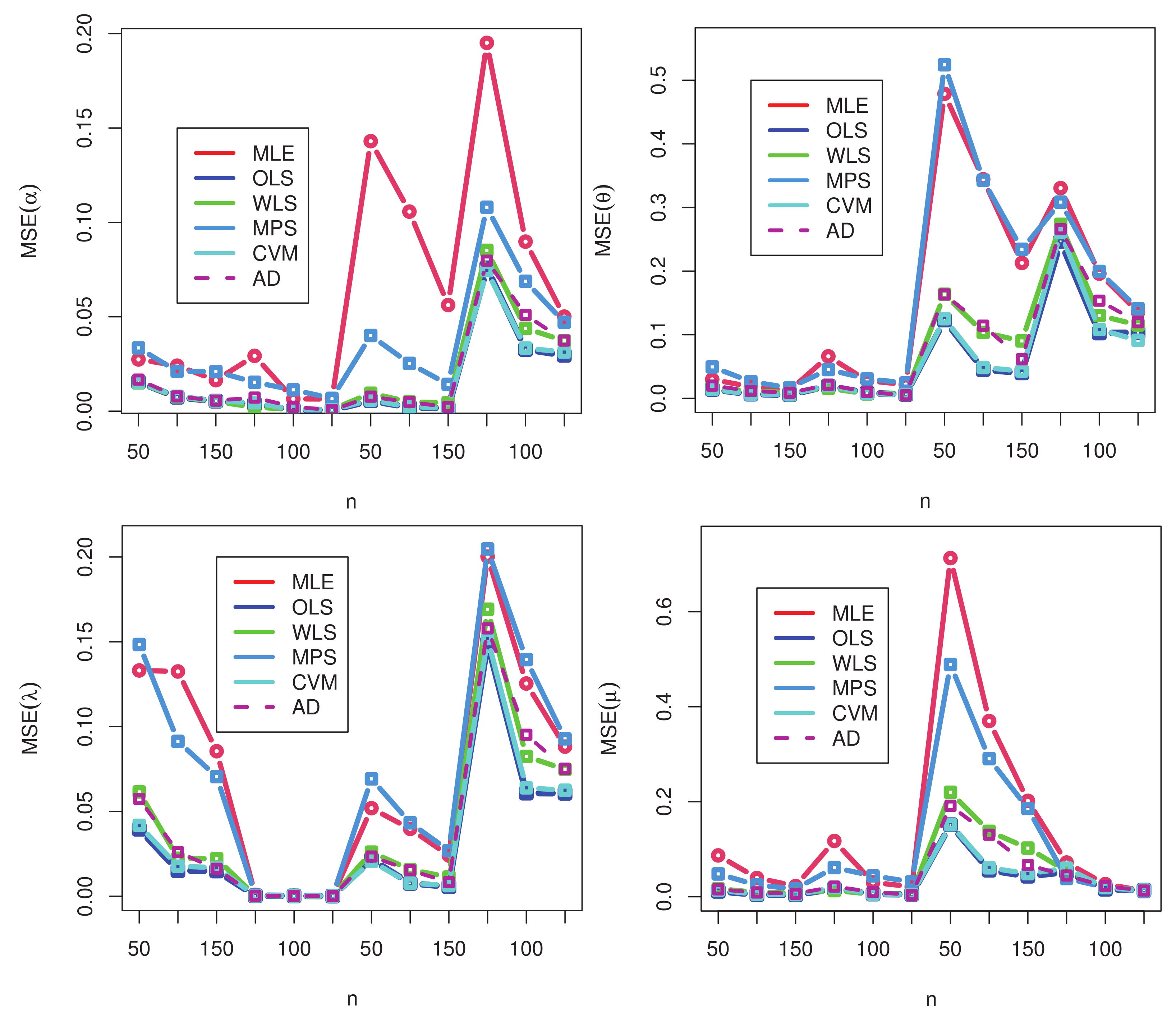
6. Numerical Outcomes

In this section, Monte Carlo simulations are run to evaluate the correctness and consistency of the new class’s six estimation methods. For the sake of example, the simulations are run with the estimators of the T I I H L O F W distribution’s parameters. The simulation replication is taken as N = 1000 and samples of sizes n = 50 , 100 and 150 are generated by using the inverse transformation,
x i = 1 λ log 1 1 1 + [ 1 α log ( U 2 U ) ] 1 θ 1 μ , i = 1 , 2 , , n ,
where U is a uniform distribution on ( 0 , 1 ) . The numerical outcomes are evaluated depending on the estimated relative biases (RB) and mean square errors (MSE). Table 4, shows the estimated RB and the MSE for the estimators of the parameters. Set four arbitrarily true values of ( α , θ , λ and μ ) such as Case I: ( α = 0.5 ; θ = 0.5 ; λ = 0.5 ; μ = 0.5 ), Case II: ( α = 1.5 ; θ = 1.5 ; λ = 0.5 ; μ = 2 ), Case III: ( α = 3 ; θ = 1.5 ; λ = 3 ; μ = 2 ), and Case IV: ( α = 3 ; θ = 1.5 ; λ = 3 ; μ = 0.5 ).
Extensive computations were carried out using the R statistical programming language software, with the most useful statistical package being the “stats” package, which used the conjugate-gradient maximization algorithm.
From Table 4, we are able to make the following observations. The performances of the proposed estimates of α , θ , λ , and μ in terms of their RB and MSE become better as n increases, as expected, where the results revealed that as the sample size increases, RB and MSE decrease. These findings clearly demonstrate the estimation methods estimators’ accuracy and consistency. As a result, the six estimation methods approach performs well in estimating the parameters of the T I I H L O F W distribution. By the results of Table 4 and Figure 5, we show the OLS method and CVM method of estimation are better than other methods.

7. Applications

Here, we provide three applications to demonstrate the adaptability of the new recommended family. Some measures of goodness of fit are used to illustrate the flexibility of the TIIHLOF-G: the values of negative LL function (−LL), KAINC (Akaike Information Criterion (INC) ), KCAINC (Akaike INC with correction), KBINC (Bayesian INC), and KHQINC (Hannon–Quinn INC) are computed for all competitive models in order to verify which distribution fits the data more closely. The best distribution has the lowest numerical values of −LL, KAINC, KCAINC, KBINC, and KHQINC.

7.1. The Biomedical Data Set

The set of data just on relief times of 20 patients who received an analgesic (Gross and Clark, 1975) is 1.50, 1.20, 2.30, 1.80, 2.20, 1.70, 1.10, 4.10, 1.80, 1.60, 1.40, 1.40, 3.00, 1.70, 1.30, 1.60, 1.70, 1.90, 2.70, 2.00.
Throughout this subsection, we apply the TIIHLOFExp model to a real-world data set to assess its adaptability. To compare the TIIHLOFExp model to the other ten fitted distributions, one, two, three, four, and five parameters are employed. We compare the TIIHLOFExp distribution with the beta transmuted Weibull (BTW), Type I half-Logistic inverse power Ailamujia (TIHLIPA), McDonald log-logistic (McLL), Marshall–Olkin exponential (M-OExp), McDonald Weibull (McW), Burr X-Ex (BrXExp), transmuted exponentiated Chen (TEC), Kumaraswamy Ex (KwExp), generalized Marshall–Olkin Ex (GM-OExp), transmuted complementary Weibull-geometric (TCWG), beta Ex (BExp), Kumaraswamy Marshall–Olkin Ex (KwM-OExp), transmuted Chen (TC), Ailamujia (A), inverse Ailamujia (IA), Exp, beta Lomax (BL), gamma-Chen (GaC), Chen (C), Weibull Lomax (WL), Kumaraswamy Chen (KwC), odd log-logistic Weibull (OLL-W), beta Weibull (BW), beta-Chen (BC), Weibull (W), and Marshall–Olkin Chen (M-OC) models. All of these competitive models are mentioned in Al-Moisheer and Alotaibi (2022).
The parameter estimates and the numerical value of negative LL are presented in Table 5. Additionally, the numerical values of KAINC, KCAINC, KBINC, and KHQINC statistics for the biomedical data are presented in Table 6.
From Table 5 and Table 6, the values of −LL, KAINC, KCAINC, KBINC, and KHQINC are minimum for the T I I H L O F E x p distribution. Thus the T I I H L O F E x p distribution is a better model for the biomedical data as compared with the other twenty-six models.

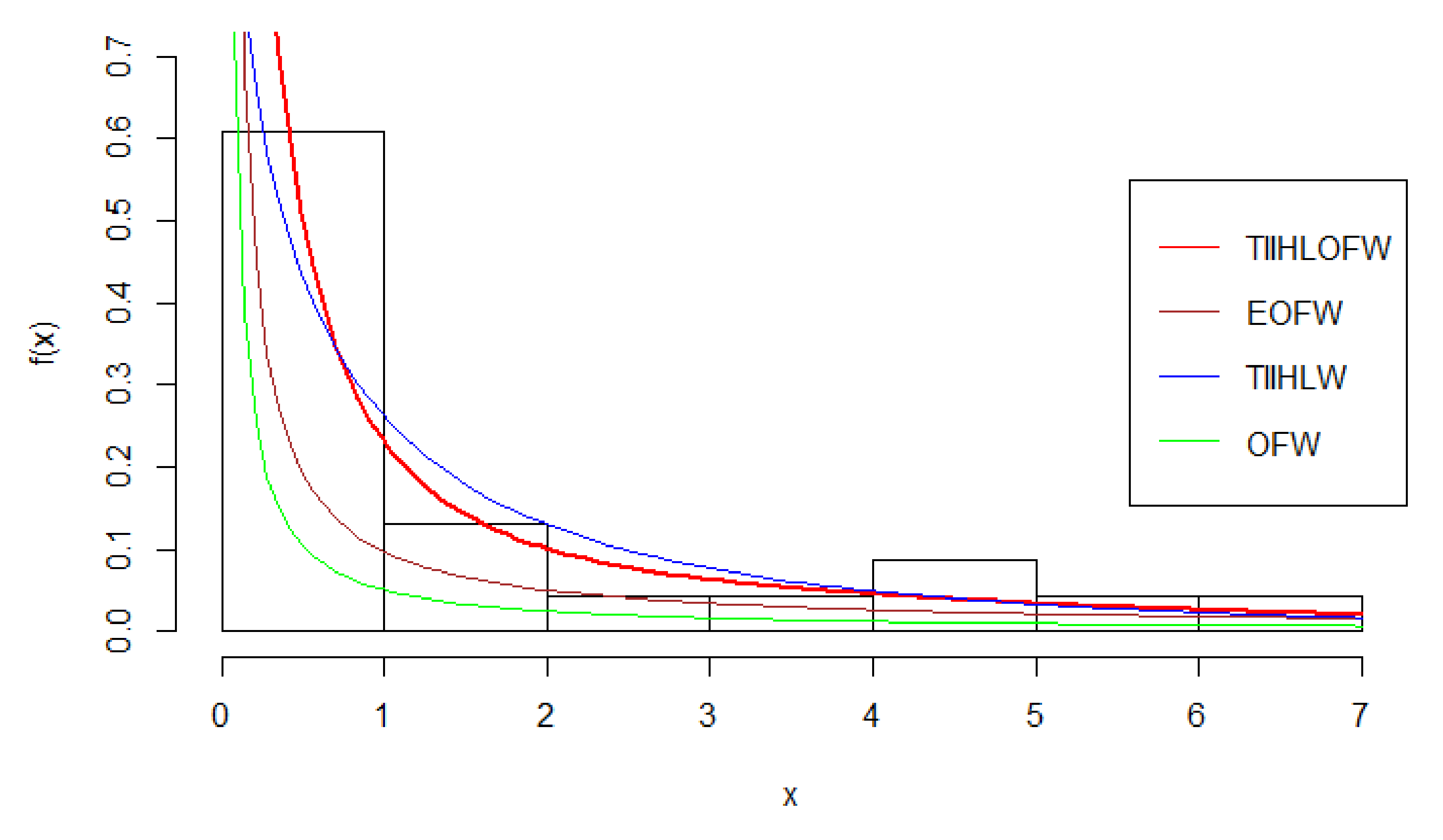
7.2. Engineering Data Set

The second data have been obtained from [34], it is for the time between failures (thousands of hours) of secondary reactor pumps. The data are as follows:
1.9210, 4.0820, 0.1990, 2.1600, 0.7460, 6.5600, 4.9920, 0.3470, 0.1500, 0.3580, 0.1010, 1.3590, 3.4650, 1.0600, 0.6140, 0.6050, 0.4020, 0.9540, 0.4910, 0.2730, 0.0700, 0.0620, 5.320.
We compare the fit of the T I I H L O F W distribution with the following continuous lifetime distributions:
(i) Extended OF Weibull (EOFW) distribution of [12] has pdf given by
f ( x ; λ , α , μ , θ ) = α θ μ λ μ x μ 1 e ( λ x ) μ [ 1 ( 1 e ( λ x ) μ ) α ] θ 1 [ 1 e ( λ x ) μ ] α θ + 1 , x > 0 .
(ii) Type II HL Weibull (TIIHLW) distribution of [28] has pdf given by
f ( x ; λ , α , μ , θ ) = 2 θ μ λ μ x μ 1 e ( λ x ) μ ( 1 e ( λ x ) μ ) θ 1 [ 1 + ( 1 e ( λ x ) μ ) θ ] 2 , x > 0 .
(iii) OF Weibull (OFW) distribution of [1] has pdf given by
f ( x ; λ , μ , θ ) = θ μ λ μ x μ 1 e ( λ x ) μ ( e ( λ x ) μ ) θ 1 e ( e ( λ x ) μ 1 e ( λ x ) μ ) θ ( 1 e ( λ x ) μ ) θ + 1 , x > 0 .
The parameter estimates and the numerical value of negative LL are presented in Table 7. Additionally, the numerical values of KAINC, KCAINC, KBINC, and KHQINC statistics for the engineering data are presented in Table 8.
From Table 7 and Table 8, the values of −LL, KAINC, KCAINC, KBINC, and KHQINC are minimum for the T I I H L O F W distribution. Thus the T I I H L O F W distribution is a better model for the engineering data as compared with the other three models. Figure 6 displays the fitted pdf plots of the engineering data set.

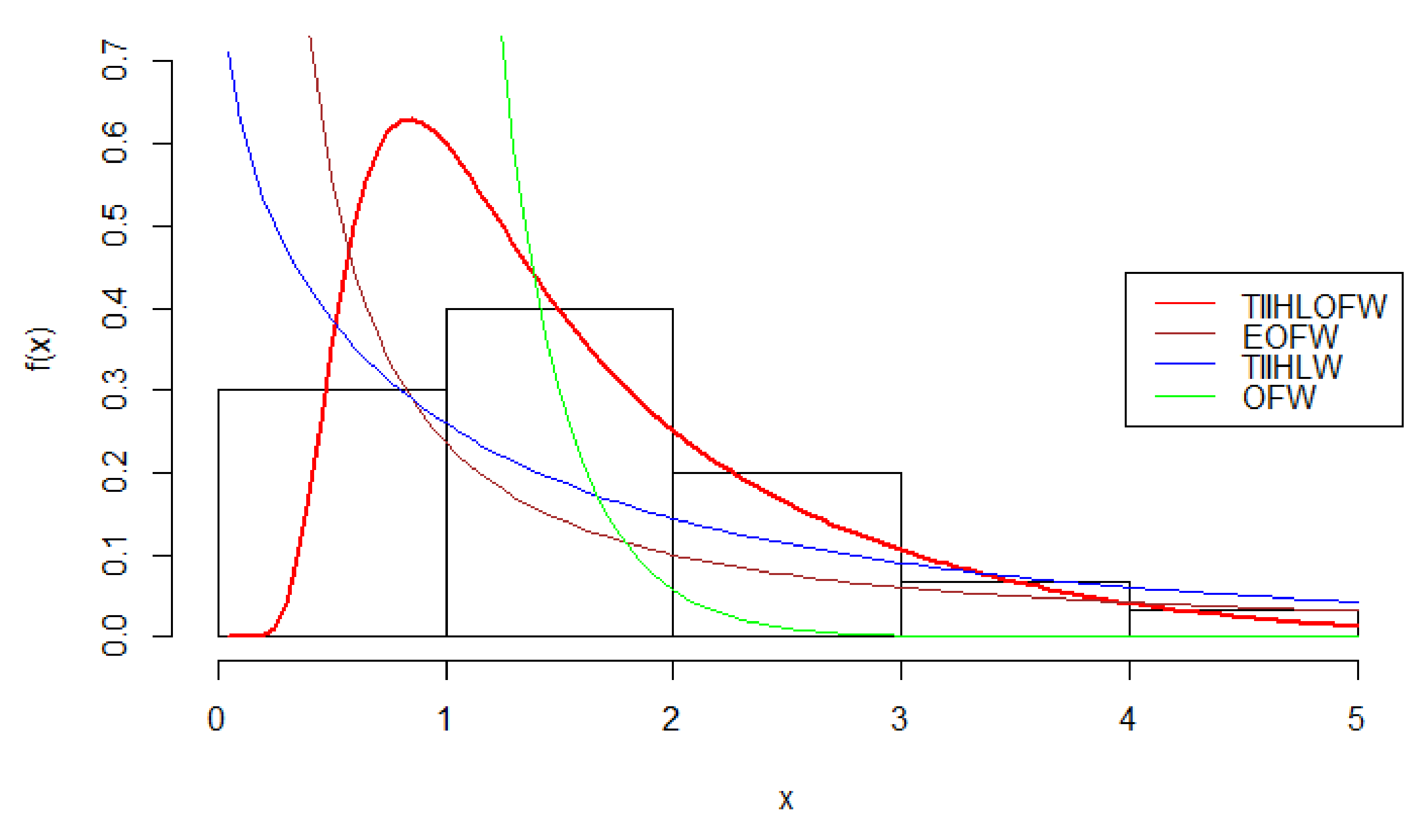
7.3. Environmental Data Set

The third data set is obtained from [35], it consists of thirty successive values of March precipitation (in inches) in Minneapolis/St Paul. The data are as follows:
1.180, 1.350, 4.750, 0.770, 1.950, 1.200, 0.470, 1.430, 3.370, 2.200, 3.000, 3.090, 1.510, 2.100, 0.520, 1.620, 1.310, 0.320, 0.590, 0.810, 2.810, 1.870, 2.480, 0.960, 1.890, 0.900, 1.740, 0.810, 1.200, 2.050.
We compare the fit of the T I I H L O F W distribution with the following continuous lifetime distributions: EOFW, TIIHLW, and OFW models.
The parameter estimates and the numerical value of negative LL are presented in Table 9. Additionally, the numerical values of KAINC, KCAINC, KBINC, and KHQINC statistics for the environmental data are presented in Table 10.
From Table 9 and Table 10, the values of −LL, KAINC, KCAINC, KBINC, and KHQINC are minimum for the T I I H L O F W distribution. Thus the T I I H L O F W distribution is a better model for the environmental data as compared with the other three models. Figure 7 displays the fitted pdf plots of the environmental data set.
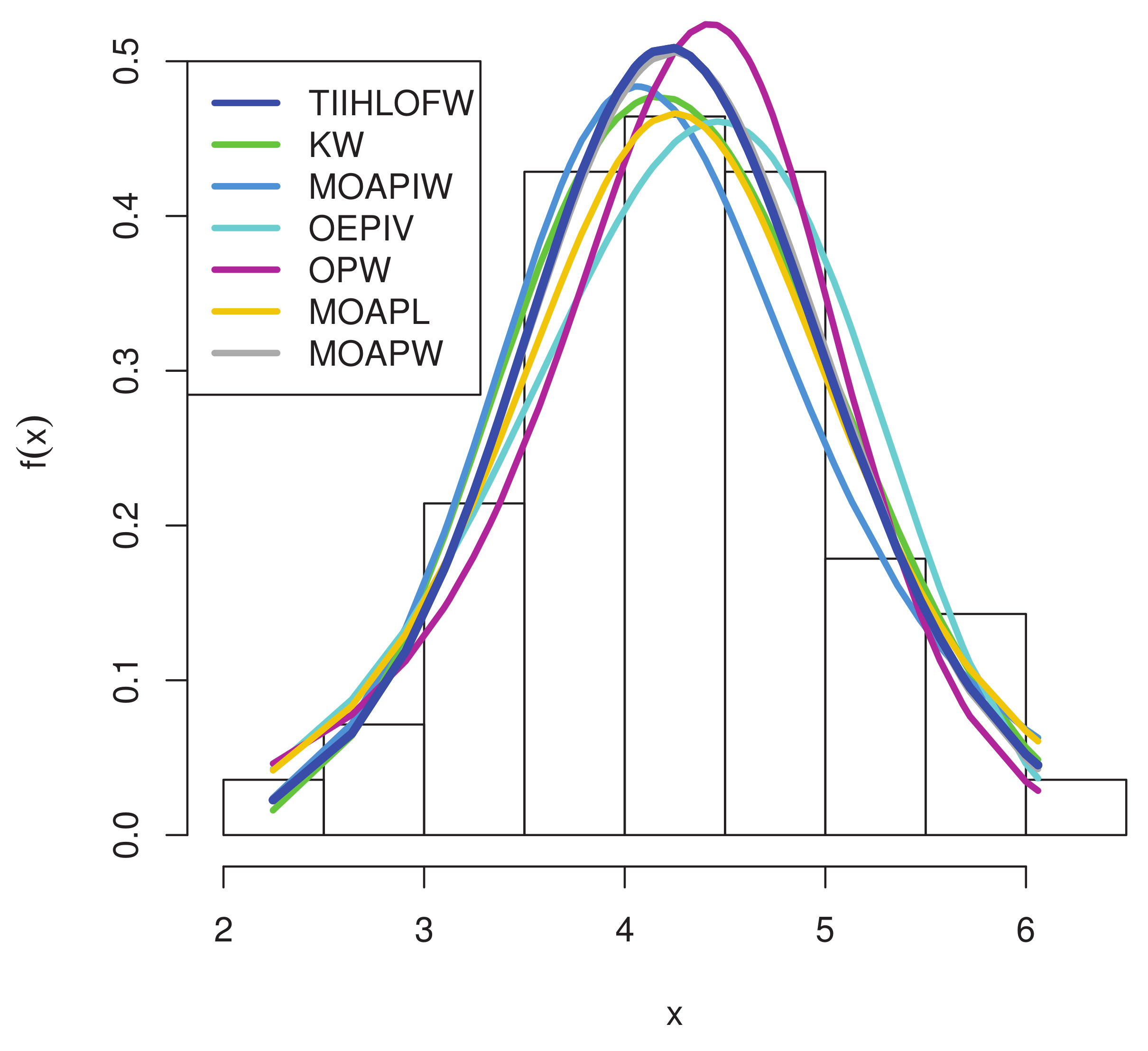
7.4. Strength Data

The fourth data set is obtained from Ahmadini et al. [36], it consists of 56 values of strength data measured in GPA, the single carbon fibers, and 1000 impregnated carbon fiber tows. The data are as follows:
2.247, 2.64, 2.908, 3.099, 3.126, 3.245, 3.328, 3.355, 3.383, 3.572, 3.581, 3.681, 3.726, 3.727, 3.728, 3.783, 3.785, 3.786, 3.896, 3.912, 3.964, 4.05, 4.063, 4.082, 4.111, 4.118, 4.141, 4.246, 4.251, 4.262, 4.326, 4.402, 4.457, 4.466, 4.519, 4.542, 4.555, 4.614, 4.632, 4.634, 4.636, 4.678, 4.698, 4.738, 4.832, 4.924, 5.043, 5.099, 5.134, 5.359, 5.473, 5.571, 5.684, 5.721, 5.998, 6.06
We compare the fit of the T I I H L O F W distribution with the following continuous lifetime distributions: Kumaraswamy Weibull (KW) by Cordeiro et al. [37], Marshall–Olkin alpha power Weibull (MOAPW) by Almetwally [38], Marshall–Olkin alpha power inverse Weibull (MOAPIW) by Basheer et al. [32], odd Perks Weibull (OPW) by Elbatal et al. [14], Marshall–Olkin alpha power Lomax (MOAPL) by Almongy et al. [33], and Odds exponential-Pareto IV (OWPIV) by Baharith et al. [39].
The parameter estimates and the numerical value of negative LL are presented in Table 11. Additionally, the numerical values of KAINC, KCAINC, KBINC, and KHQINC statistics for the environmental data are presented in Table 12.
From Table 11 and Table 12, the values of −LL, KAINC, KCAINC, KBINC, and KHQINC are minimum for the T I I H L O F W distribution. Thus the T I I H L O F W distribution is a better model for the environmental data as compared with the other three models. Figure 8 displays the fitted pdf plots of the strength data set.

8. Conclusions and Summary

We presented a new class of continuous distributions entitled the Type II half-Logistic odd Fréchet-G class in this work. The identifiability of the proposed model was proved and also studied its relationship with other families of distributions. Some statistical properties such as ORMs, INMs, MGEF, REL, RREL, and entropy are derived. The estimates of the parameters of the new model are estimated using the ML method. A simulation outcome was conducted to check the performance of the MLE method. Using four real-life data sets we illustrated the flexibility of the TIIHLOFExp and TIIHLOFW models. In our future works, the new suggested class of distributions will be used to generate more new statistical models, the statistical features of which will be explored. We also intend to study the statistical inferences of new models generated using the TIIHLOF-G class.

Author Contributions

Conceptualization, I.E.; methodology, I.E. and M.G.B.; software and M.E.; validation, N.A., S.A.A., M.E. and I.E.; formal analysis, M.G.B.; resources, I.E.; data curation, I.E., N.A. and S.A.A.; writing—original draft preparation, I.E. and M.E.; writing—review and editing, N.A., S.A.A. and M.E.; funding acquisition, I.E., N.A. and S.A.A. All authors have read and agreed to the published version of the manuscript.

Funding

The authors extend their appreciation to the Deanship of Scientific Research at Imam Mohammad Ibn Saud Islamic University for funding this work through Research Group no. RG-21-09-15.

Informed Consent Statement

Informed consent was obtained from all subjects involved in the study.

Data Availability Statement

Data sets are available in the application section.

Acknowledgments

The authors extend their appreciation to the Deanship of Scientific Research at Imam Mohammad Ibn Saud Islamic University for funding this work through Research Group no. RG-21-09-15.

Conflicts of Interest

The authors declare no conflict of interest.

References

  1. Haq, A.; Elgarhy, M. The odd Fréchet-G class of probability distributions. J. Stat. Appl. Probab. 2018, 7, 189–203. [Google Scholar] [CrossRef]
  2. Marshall, A.; Olkin, I. A new method for adding a parameter to a class of distributions with applications to the exponential and Weibull families. Biometrika 1997, 84, 641–652. [Google Scholar] [CrossRef]
  3. Eugene, N.; Lee, C.; Famoye, F. Beta-normal distribution and its applications. Commun. Stat. Theory Methods 2002, 31, 497–512. [Google Scholar] [CrossRef]
  4. Gleaton, J.U.; Lynch, J.D. Properties of generalized log-logistic families of lifetime distributions. J. Probab. Stat. Sci. 2006, 4, 51–64. [Google Scholar]
  5. Afify, A.Z.; Altun, E.; Alizadeh, M.; Ozel, G.; Hamedani, G.G. The odd exponentiated half-logistic-G class: Properties, characterizations and applications. Chil. J. Stat. 2017, 8, 65–91. [Google Scholar]
  6. Cordeiro, G.M.; Alizadeh, M.; Ozel, G.; Hosseini, B.; Ortega, E.M.M.; Altun, E. The generalized odd log-logistic class of distributions: Properties, regression models and applications. J. Stat. Comput. Simul. 2017, 87, 908–932. [Google Scholar] [CrossRef]
  7. Cordeiro, G.M.; Alizadeh, M.; Diniz Marinho, P.R. The type I half-logistic class of distributions. J. Stat. Comput. Simul. 2015, 86, 707–728. [Google Scholar] [CrossRef]
  8. Tahir, M.H.; Cordeiro, G.M.; Alzaatreh, A.; Mansoor, M.; Zubair, M. The Logistic-X class of distributions and its Applications. Commun. Stat. Theory Method 2016, 45, 7326–7349. [Google Scholar] [CrossRef] [Green Version]
  9. Haghbin, H.; Ozel, G.; Alizadeh, M.; Hamedani, G.G. A new generalized odd log-logistic class of distributions. Commun. Stat. Theory Methods 2017, 46, 9897–9920. [Google Scholar] [CrossRef]
  10. El-Sherpieny, E.; EL-Sehetry, M. Kumaraswamy Type I Half-logistic class of Distributions with Applications. Gazi Univ. J. Sci. 2019, 32, 333–349. [Google Scholar]
  11. Badr, M.; Elbatal, I.; Jamal, F.; Chesneau, C.; Elgarhy, M. The Transmuted Odd Fréchet-G class of Distributions: Theory and Applications. Mathematics 2020, 8, 958. [Google Scholar] [CrossRef]
  12. Nasiru, S. Extended Odd Fréchet-G class of Distributions. J. Probab. Stat. 2018, 2018, 2931326. [Google Scholar] [CrossRef]
  13. Afify, A.Z.; Alizadeh, M.; Yousof, H.M.; Aryal, G.; Ahmad, M. The transmuted geometric-G family of distributions: Theory and applications. Pak. J. Stat. 2016, 32, 139–160. [Google Scholar]
  14. Elbatal, I.; Alotaibi, N.; Almetwally, E.M.; Alyami, S.A.; Elgarhy, M. On Odd Perks-G Class of Distributions: Properties, Regression Model, Discretization, Bayesian and Non-Bayesian Estimation, and Applications. Symmetry 2022, 14, 883. [Google Scholar] [CrossRef]
  15. Gomes, F.; Percontini, A.; de Brito, E.; Ramos, M.; Venancio, R.; Cordeiro, G. The odd Lindley-G family of distributions. Austrian J. Stat. 2017, 1, 57–79. [Google Scholar]
  16. Alotaibi, N.; Elbatal, I.; Almetwally, E.M.; Alyami, S.A.; Al-Moisheer, A.S.; Elgarhy, M. Truncated Cauchy Power Weibull-G Class of Distributions: Bayesian and Non-Bayesian Inference Modelling for COVID-19 and Carbon Fiber Data. Mathematics 2022, 10, 1565. [Google Scholar] [CrossRef]
  17. Nofal, Z.M.; Afify, A.Z.; Yousof, H.M.; Cordeiro, G.M. The generalized transmuted-G family of distributions. Commun. Stat. Theory Methods 2017, 46, 4119–4136. [Google Scholar] [CrossRef]
  18. Aldahlan, M.A.; Jamal, F.; Chesneau, C.; Elgarhy, M.; Elbatal, I. The truncated Cauchy power family of distributions with inference and applications. Entropy 2020, 22, 346. [Google Scholar] [CrossRef] [Green Version]
  19. Yousof, H.M.; Afify, A.Z.; Hamedani, G.G.; Aryal, G. The Burr X generator of distributions for lifetime data. J. Stat. Theory Appl. 2017, 16, 288–305. [Google Scholar] [CrossRef] [Green Version]
  20. Al-Moisheer, A.S.; Elbatal, I.; Almutiry, W.; Elgarhy, M. Odd inverse power generalized Weibull generated family of distributions: Properties and applications. Math. Probl. Eng. 2021, 2021, 5082192. [Google Scholar] [CrossRef]
  21. Al-Mofleh, H.; Elgarhy, M.; Afify, A.Z.; Zannon, M.S. Type II exponentiated half logistic generated family of distributions with applications. Electron. J. Appl. Stat. Anal. 2020, 13, 36–561. [Google Scholar]
  22. Al-Shomrani, A.; Arif, O.; Shawky, A.; Hanif, S.; Shahbaz, M.Q. Topp–Leone family of distributions: Some properties and application. Pak. J. Stat. Oper. Res. 2016, 12, 443–451. [Google Scholar] [CrossRef] [Green Version]
  23. Bantan, R.A.; Chesneau, C.; Jamal, F.; Elgarhy, M. On the analysis of new COVID-19 cases in Pakistan using an exponentiated version of the M family of distributions. Mathematics 2020, 8, 953. [Google Scholar] [CrossRef]
  24. Nascimento, A.; Silva, K.F.; Cordeiro, M.; Alizadeh, M.; Yousof, H.; Hamedani, G. The odd Nadarajah–Haghighi family of distributions. Prop. Appl. Stud. Sci. Math. Hung. 2019, 56, 1–26. [Google Scholar]
  25. Almarashi, A.M.; Jamal, F.; Chesneau, C.; Elgarhy, M. The Exponentiated truncated inverse Weibull-generated family of distributions with applications. Symmetry 2020, 12, 650. [Google Scholar] [CrossRef] [Green Version]
  26. Alzaatreh, A.; Lee, C.; Famoye, F. A new method for generating families of continuous distributions. Metron 2013, 71, 63–79. [Google Scholar] [CrossRef] [Green Version]
  27. Jayakumar, K.; Babu, M.G. A new generalization of the Fréchet distribution: Properties and application. Statistica 2019, 79, 267–289. [Google Scholar]
  28. Hassan, A.S.; Elgarhy, M.; Shakil, M. Type II half-logistic class of distributions with applications. Pak. J. Stat. Oper. Res. 2017, 13, 245–264. [Google Scholar]
  29. Ibrahim, G.M.; Hassan, A.S.; Almetwally, E.M.; Almongy, H.M. Parameter estimation of alpha power inverted Topp–Leone distribution with applications. Intell. Autom. Soft Comput. 2021, 29, 353–371. [Google Scholar] [CrossRef]
  30. Almetwally, E.M. The odd Weibull inverse topp–leone distribution with applications to COVID-19 data. Ann. Data Sci. 2022, 9, 121–140. [Google Scholar] [CrossRef]
  31. Almetwally, E.M.; Ahmad, H.H. A new generalization of the Pareto distribution and its applications. Stat. Transit. New Ser. 2020, 21, 61–84. [Google Scholar] [CrossRef]
  32. Basheer, A.M.; Almetwally, E.M.; Okasha, H.M. Marshall-olkin alpha power inverse Weibull distribution: Non bayesian and bayesian estimations. J. Stat. Appl. Probab. 2021, 10, 327–345. [Google Scholar]
  33. Almongy, H.M.; Almetwally, E.M.; Mubarak, A.E. Marshall–Olkin alpha power lomax distribution: Estimation methods, applications on physics and economics. Pak. J. Stat. Oper. Res. 2021, 17, 137–153. [Google Scholar] [CrossRef]
  34. Salman, S.M.; Sangadji, P. Total time on test plot analysis for mechanical components of the RSG-GAS reactor. Atom Indones 1999, 25, 155–161. [Google Scholar]
  35. Hinkley, D. On quick choice of power transformations. J. R. Stat. Soc. Ser. Appl. Stat. 1977, 26, 67–69. [Google Scholar] [CrossRef]
  36. Ahmadini, A.A.H.; Hassan, A.S.; Mohamed, R.E.; Alshqaq, S.S.; Nagy, H.F. A New four-parameter moment exponential model with applications to lifetime data. Intell. Autom. Soft Comput. 2021, 29, 131–146. [Google Scholar] [CrossRef]
  37. Cordeiro, G.M.; Ortega, E.M.; Nadarajah, S. The Kumaraswamy Weibull distribution with application to failure data. J. Frankl. Inst. 2010, 347, 1399–1429. [Google Scholar] [CrossRef]
  38. Almetwally, E.M. Marshall olkin alpha power extended Weibull distribution: Different methods of estimation based on type i and type II censoring. Gazi Univ. J. Sci. 2022, 35, 293–312. [Google Scholar]
  39. Baharith, L.A.; Al-Beladi, K.M.; Klakattawi, H.S. The Odds exponential-pareto IV distribution: Regression model and application. Entropy 2020, 22, 497. [Google Scholar] [CrossRef]
Figure 1. Shapes of the pdf of TIIHLOFExp ( α , λ , θ ) for various values of parameter.
Symmetry 14 01222 g001
Figure 2. Shapes of the pdf of TIIHLOFR ( α , β , θ ) for various values of parameter.
Symmetry 14 01222 g002
Figure 3. Shapes of the pdf of TIIHLOFW ( α , λ , μ , θ ) for various values of parameter.
Symmetry 14 01222 g003
Figure 4. Shapes of the pdf of TIIHLOFL ( α , λ , θ ) for various values of parameter.
Symmetry 14 01222 g004
Figure 5. MSE with different sample sizes.
Symmetry 14 01222 g005
Figure 6. Fitted pdf for the engineering data set.
Symmetry 14 01222 g006
Figure 7. Fitted pdf for the environmental data.
Symmetry 14 01222 g007
Figure 8. Fitted pdf for the strength data.
Symmetry 14 01222 g008
Table 1. Numerical values of E ( X ) , E ( X 2 ) , E ( X 3 ) , E ( X 4 ) , Var(X), SK, KU, and CV of the T I I H L O F E x p distribution.
α λ θ E ( X ) E ( X 2 ) E ( X 3 ) E ( X 4 ) Var(X)SKKUCV
0.50.50.51.3868.64798.1101546.2036.7263.8683.8681.871
0.91.1833.39418.738154.5871.9943.5523.5521.193
1.51.1772.0685.79524.7880.6843.0993.0990.703
0.90.50.7702.66916.823147.2912.0763.8683.8681.871
0.90.6571.0483.21314.7260.6163.5523.5521.193
1.50.6540.6380.9942.3610.2113.0993.0990.703
1.50.50.4620.9613.63419.0890.7473.8683.8681.871
0.90.3940.3770.6941.9080.2223.5523.5521.193
1.50.3920.2300.2150.3060.0763.1003.1000.703
0.90.50.52.28615.368176.1182781.12510.1442.9292.9291.393
0.91.7365.82733.439277.7372.8132.8722.8720.966
1.51.5313.2399.97544.1190.8942.6932.6930.617
0.90.51.2704.74330.199264.9303.1312.9292.9291.393
0.90.9641.7985.73026.4570.8682.8682.8680.966
1.50.8511.0001.7104.2030.2762.6932.6930.617
1.50.50.7621.7086.52334.3351.1272.9292.9291.393
0.90.5790.6471.2383.4290.3132.8682.8680.966
1.50.5100.3600.3690.5450.0992.6932.6930.617
1.50.50.53.39524.984291.6924626.89013.4602.3392.3391.081
0.92.3519.11954.810461.0693.5902.4242.4240.806
1.51.8954.68315.75372.3311.0912.4082.4080.551
0.90.51.8867.71150.016440.7574.1542.3392.3391.081
0.91.3062.8149.39843.9211.1082.4242.4240.806
1.51.0531.4452.7016.8900.3372.4082.4080.551
1.50.51.1322.77610.80357.1221.4962.3392.3391.081
0.90.7841.0132.0305.6920.3992.4242.4240.806
1.50.6320.5200.5830.8930.1212.4082.4080.551
Table 2. Numerical values of E ( X ) , E ( X 2 ) , E ( X 3 ) , E ( X 4 ) , Var(X), SK, KU, and CV of the T I I H L O F R distribution.
α λ θ E ( X ) E ( X 2 ) E ( X 3 ) E ( X 4 ) Var(X)SKKUCV
0.50.50.51.2602.7728.78634.5881.1841.7931.7930.863
0.91.3742.3675.12213.5780.4781.6841.6840.503
1.51.4692.3534.1708.2740.1951.6291.6290.300
0.90.50.9391.5403.63810.6750.6581.7931.7930.863
0.91.0241.3152.1214.1910.2661.6841.6840.503
1.51.0951.3071.7272.5540.1081.6291.6290.300
1.50.50.7280.9241.6913.8430.3951.7931.7930.863
0.90.7930.7890.9861.5090.1591.6841.6840.503
1.50.8480.7840.8030.9190.0651.6291.6290.300
0.90.50.51.7774.57115.31961.4701.4121.2951.2950.669
0.91.7143.4728.32223.3090.5341.3841.3840.426
1.51.6893.0636.02312.9570.2101.4631.4630.271
0.90.51.3252.5406.34318.9720.7851.2951.2950.669
0.91.2781.9293.4467.1940.2971.3841.3840.426
1.51.2591.7022.4943.9990.1171.4631.4630.271
1.50.51.0261.5242.9486.8300.4711.2951.2950.669
0.90.9901.1571.6022.5900.1781.3841.3840.426
1.50.9751.0211.1591.4400.0701.4631.4630.271
1.50.50.52.3046.78924.22399.9351.4830.9700.9700.529
0.92.0364.70212.32736.4740.5551.1801.1800.366
1.51.8903.7908.12418.7310.2181.3431.3430.247
0.90.51.7173.77210.03030.8440.8240.9700.9700.529
0.91.5182.6125.10411.2570.3091.1801.1800.366
1.51.4092.1063.3645.7810.1211.3431.3430.247
1.50.51.3302.2634.66211.1040.4940.9700.9700.529
0.91.1761.5672.3724.0530.1851.1801.1800.366
1.51.0911.2631.5632.0810.0731.3431.3430.247
Table 3. Numerical values of E ( X ) , E ( X 2 ) , E ( X 3 ) , E ( X 4 ) , Var(X), SK, KU, and CV of the T I I H L O F L distribution.
α λ θ E ( X ) E ( X 2 ) E ( X 3 ) E ( X 4 ) Var(X)SKKUCV
0.50.50.52.26016.846217.9063836.06811.7403.1523.1521.516
0.92.1678.63657.738554.2103.9402.8062.8060.916
1.52.2566.55325.753138.0651.4632.4692.4690.536
0.90.51.1464.73533.986331.4283.4223.2733.2731.614
0.91.0682.2768.40444.7291.1352.9352.9350.997
1.51.1021.6343.42410.0650.4192.5792.5790.587
1.50.50.6331.5506.63238.5911.1503.4053.4051.695
0.90.5740.7031.5364.8670.3733.0863.0861.065
1.50.5860.4790.5760.9970.1362.7192.7190.630
0.90.50.53.59529.612390.0036893.54716.6872.3992.3991.136
0.93.02214.300101.607991.8295.1652.3142.3140.752
1.52.8109.68142.469240.6721.7852.1952.1950.475
0.90.51.8498.35660.885595.7444.9382.4762.4761.202
0.91.5183.82014.86580.1681.5142.3972.3970.810
1.51.3952.4665.73817.6920.5192.2722.2720.516
1.50.51.0302.74211.88969.3811.6822.5682.5681.260
0.90.8261.1902.7268.7310.5072.5022.5020.862
1.50.7500.7340.9761.7610.1722.3732.3730.552
1.50.50.55.14747.337642.10911444.72420.8481.9321.9320.887
0.93.92021.553163.6391635.4626.1871.9911.9910.635
1.53.35313.30364.309385.1662.0582.0002.0000.428
0.90.52.68013.430100.417989.6236.2481.9811.9810.933
0.91.9985.83024.091132.5051.8372.0472.0470.678
1.51.6853.4468.81528.5640.6052.0572.0570.462
1.50.51.5064.42519.635115.3072.1562.0452.0450.975
0.91.1001.8344.43814.4550.6242.1232.1230.718
1.50.9151.0401.5162.8620.2032.1352.1350.492
Table 4. The MLE, OLS, WLS, MPS, CVM, and AD estimated RB and MSE of the T I I H L O F W distribution.
MLEOLSWLSMPSCVMAD
Casen RBMSERBMSERBMSERBMSERBMSERBMSE
I50 α 0.09000.02740.02890.01540.02960.01500.08970.03350.00390.01530.02800.0167
θ 0.08230.02960.01200.01420.03550.01880.08260.0494−0.00430.01420.03640.0201
λ 0.13660.13310.04880.03950.05450.06150.13570.14840.08010.04180.08750.0574
μ 0.02800.08700.02470.01150.02090.01690.02780.04800.07770.01390.02790.0155
100 α 0.06860.02410.01040.00740.00620.00760.06870.0211−0.00240.00780.01180.0078
θ 0.06480.01830.00770.00660.02630.01050.06510.02620.00150.00660.03010.0115
λ 0.10860.13250.00910.01510.00380.02240.10840.09130.02400.01770.03400.0260
μ −0.01690.03950.00670.00460.00650.0091−0.01710.02470.03020.00510.00660.0090
150 α 0.04960.01640.00590.0053−0.00070.00510.06200.02100.00020.00540.00470.0056
θ 0.04250.01260.00580.00570.01740.00990.04290.0165−0.00140.00560.02180.0088
λ 0.09150.08550.00910.01490.00370.02210.09150.07050.02370.01690.01380.0162
μ −0.01530.02250.00600.00390.00520.0081−0.01630.01650.03010.00450.00620.0063
II50 α 0.00300.02930.00280.00370.00250.00210.00290.01530.00750.00450.00780.0072
θ −0.01220.0660−0.00820.0194−0.00110.0158−0.01230.04520.00750.01990.00090.0212
λ −0.00660.0008−0.00220.0003−0.00210.0003−0.00670.0006−0.00040.0003−0.00080.0003
μ −0.01780.11740.00090.01680.00270.0129−0.01800.06140.01430.01910.00780.0214
100 α −0.00240.0065−0.00140.00070.00040.0010−0.00250.01130.00140.00080.00150.0023
θ 0.00410.0277−0.00620.0083−0.00110.00710.00410.03070.00040.0077−0.00080.0099
λ −0.00550.0003−0.00020.00020.00050.0002−0.00550.00040.00090.00020.00050.0002
μ −0.01720.0301−0.00040.0057−0.00010.0057−0.01720.04390.00320.00560.00060.0100
150 α −0.00240.0064−0.00120.0006−0.00040.0009−0.00240.00680.00040.0007−0.00040.0006
θ 0.00400.0217−0.00030.00620.00110.00700.00400.02410.00030.00570.00070.0049
λ −0.00530.0002−0.00010.0001−0.00030.0001−0.00540.00030.00070.00010.00020.0001
μ −0.01290.0211−0.00040.0051−0.00010.0057−0.01490.03140.00130.0046−0.00060.0040
III50 α 0.02010.14300.00560.00550.00780.00950.02000.04010.00820.00590.00870.0077
θ 0.11000.4787−0.00420.12310.01050.16360.11070.5244−0.00110.12520.01670.1633
λ −0.00900.05190.00370.02170.00140.0260−0.00920.06920.00280.0205−0.00020.0234
μ −0.01110.71290.02980.15150.03300.2199−0.01190.48880.05680.15180.03560.1916
100 α 0.01480.10570.00120.00210.00370.00490.01470.02530.00190.00220.00390.0048
θ 0.09770.3444−0.00420.04520.00410.10360.09780.34280.00100.04850.01370.1142
λ −0.00810.03970.00330.00760.00130.0157−0.00810.04330.00170.00770.00020.0153
μ −0.01030.36990.00700.05590.02050.1377−0.01130.29070.01590.06100.01750.1306
150 α 0.01070.05620.00020.00150.00330.00450.01080.01420.00100.00170.00140.0022
θ 0.08480.21280.00310.04000.00400.09020.08620.23430.00100.04280.01200.0615
λ −0.00800.02400.00010.0057−0.00090.0113−0.00810.0269−0.00050.0063−0.00020.0083
μ −0.01060.2019−0.00140.04330.00380.1024−0.01060.18580.00720.04860.00120.0668
IV50 α 0.00620.1951−0.01120.0759−0.01060.08520.00640.1080−0.01400.0745−0.00640.0797
θ 0.02720.3304−0.02300.2467−0.02300.27350.02740.3084−0.03620.2605−0.02000.2659
λ −0.01290.20020.00640.14920.00590.1692−0.01310.20470.00910.15190.00500.1579
μ 0.05090.07200.12890.05210.13820.05430.05020.03840.18050.06010.13500.0447
100 α 0.00620.0898−0.00440.0327−0.00730.04390.00570.0688−0.00770.0334−0.00590.0510
θ 0.02610.19600.00690.1027−0.00640.13010.02370.1994−0.01180.1083−0.01320.1535
λ −0.01010.12540.00180.06080.00350.0824−0.01020.13950.00570.06390.00470.0952
μ 0.00800.02660.03300.01590.05580.02020.00770.01990.06350.01910.07350.0223
150 α 0.00600.0501−0.00270.0296−0.00200.03730.00460.0471−0.00320.03130.00070.0374
θ 0.02510.13550.00580.10320.00590.11540.01610.14090.00590.09110.01270.1197
λ −0.00930.0882−0.00060.0607−0.00170.0748−0.01010.0928−0.00060.0625−0.00450.0752
μ −0.00730.01260.03090.01380.03500.0136−0.00690.01070.04400.01390.03000.0130
Table 5. The parameter estimates and the numerical values of −LL of the biomedical data.
ModelML Estimates−LL
TIIHLOFExp α ^ = 0.052 , λ ^ = 0.179 , θ ^ = 2.973 15.392
BTW α ^ = 5.619 , β ^ = 0.531 , a ^ = 53.344 , b ^ = 3.568 , λ ^ = 0.772 16.831
TIHLIPA α ^ = 0.246 , β ^ = 4.713 , γ ^ = 6.781 16.095
McLL α ^ = 0.881 , β ^ = 2.070 , a ^ = 19.225 , b ^ = 32.033 , c ^ = 1.926 16.526
M-OExp α ^ = 54.474 , β ^ = 2.316 19.755
McW α ^ = 2.774 , β ^ = 0.380 , a ^ = 79.108 , b ^ = 17.898 , c ^ = 3.006 16.927
BrXExp α ^ = 1.164 , β ^ = 0.321 22.050
TEC α ^ = 300.010 , β ^ = 0.500 , a ^ = 2.430 , b ^ = 0.340 15.780
KwExp a ^ = 83.756 , b ^ = 0.568 , β ^ = 3.333 17.890
GM-OExp λ ^ = 0.519 , α ^ = 89.462 , β ^ = 3.169 18.375
TCWG α ^ = 43.663 , β ^ = 5.127 , γ ^ = 0.282 , λ ^ = 0.271 16.587
BExp a ^ = 81.633 , b ^ = 0.542 , β ^ = 3.514 18.740
KwM-OExp α ^ = 8.868 , β ^ = 4.899 , a ^ = 34.826 , b ^ = 0.299 17.400
TC α ^ = 0.750 , a ^ = 0.070 , b ^ = 1.020 23.815
A β ^ = 0.950 26.160
IA β ^ = 3.449 25.827
Exp β ^ = 0.526 32.835
BL a ^ = 41.070 , b ^ = 1.929 , θ ^ = 5.774 , λ ^ = 0.429 16.110
GaC α ^ = 7.590 , β ^ = 1.990 , a ^ = 5.000 , b ^ = 0.530 23.175
C a ^ = 0.140 , b ^ = 0.950 24.570
WL a ^ = 14.739 , b ^ = 5.585 , θ ^ = 0.263 , λ ^ = 0.219 19.631
KwC α ^ = 160.070 , β ^ = 0.490 , a ^ = 2.210 , b ^ = 0.520 16.010
OLL-W α ^ = 31.414 , λ ^ = 0.134 , θ ^ = 26.771 16.551
BW α ^ = 0.831 , β ^ = 0.613 , a ^ = 29.947 , b ^ = 11.632 16.804
BC α ^ = 85.870 , β ^ = 0.480 , a ^ = 2.010 , b ^ = 0.55 16.255
W λ ^ = 0.002 , θ ^ = 1.435 20.586
M-OC α ^ = 400.010 , a ^ = 2.320 , b ^ = 0.430 19.440
Table 6. The numerical values of KAINC, KCAINC, KBINC, and KHQINC statistics for the biomedical data.
ModelsKAINCKCAINCKBINCKHQINC
TIIHLOFExp36.78438.28434.68837.368
BTW43.66250.12439.46844.828
TIHLIPA38.18939.11236.09238.772
McLL43.05147.33739.55644.023
M-OExp43.5145.5144.2243.9
McW43.85448.1440.35944.826
BrXExp48.150.148.848.5
TEC39.5642.22736.76440.338
KwExp41.7844.7543.2842.32
GM-OExp42.7545.7444.2543.34
TCWG51.17355.45947.67852.145
BExp43.4846.4544.9844.02
KwM-OExp42.846.8445.5543.6
TC53.6355.1351.53354.213
A54.3255.3154.5454.5
IA53.65353.88852.95453.847
Exp67.6768.6767.8967.87
BL40.21942.88637.42340.997
GaC46.3549.01743.55447.128
C53.1453.84651.74253.529
WL47.26149.92844.46548.039
KwC40.0242.68737.22440.798
OLL-W39.10140.60137.00439.684
BW41.60744.27438.81142.385
BC40.5143.17737.71441.288
W45.172845.878645.561547.1642
M-OC44.8846.3842.78345.463
Table 7. The parameter estimates and the numerical values of −LL of the engineering data.
ModelML Estimates−LL
TIIHLOFW λ ^ = 0.3901 , α ^ = 0.5884 , μ ^ = 1.4299 , θ ^ = 0.3758 30.759
EOFW λ ^ = 0.5436 , α ^ = 0.9057 , μ ^ = 0.3694 , θ ^ = 0.1980 45.418
TIIHLW λ ^ = 0.3474 , μ ^ = 0.8837 , θ ^ = 0.9501 32.574
OFW λ ^ = 0.0464 , μ ^ = 0.0575 , θ ^ = 0.7175 60.544
Table 8. The numerical values of KAINC, KCAINC, KBINC, and KHQINC statistics for the engineering data.
ModelsKAINCKCAINCKBINCKHQINC
TIIHLOFW69.51971.74174.06170.661
EOFW98.836101.058103.37899.978
TIIHLW71.14772.41074.55472.004
OFW127.087128.350130.494127.944
Table 9. The parameter estimates and the numerical values of −LL of the environmental data.
ModelML Estimates−LL
TIIHLOFW λ ^ = 0.5477 , α ^ = 0.9205 , μ ^ = 1.8387 , θ ^ = 0.6241 38.944
EOFW λ ^ = 0.2927 , α ^ = 0.8943 , μ ^ = 0.2182 , θ ^ = 1.0587 55.876
TIIHLW λ ^ = 0.2675 , μ ^ = 0.9643 , θ ^ = 0.9297 50.921
OFW λ ^ = 0.9615 , μ ^ = 1.5339 , θ ^ = 1.5469 50.501
Table 10. The numerical values of KAINC, KCAINC, KBINC, and KHQINC statistics for the environmental data.
ModelsKAINCKCAINCKBINCKHQINC
TIIHLOFW85.88787.48791.49287.680
EOFW119.752121.352125.357121.545
TIIHLW107.842108.765112.046109.187
OFW107.002107.925111.205108.346
Table 11. The parameter estimates and the numerical values of −LL of the strength data.
ModelML Estimates−LL
TIIHLOFW α = 5.2701,0.3450 θ = 0.373, μ = 3.2985,67.7818
MOAPL α = 281.8156, β = 270.1004, θ = 550.4996, λ = 140.7209,69.1317
MOAPW α = 44.4414, β = 7.5156, θ = 0.0101, λ = 5.7759,67.9200
OPW β = 0.0101, θ = 0.1355, λ = 0.3678, δ = 0.5165,70.2290
KW α = 0.008, β = 4.1936, a = 2.8883, b = 0.2909,67.9350
MOAPIW α = 10.5695, β = 7.9752, θ = 353.0412, λ = 100.1504,69.3700
OEPIV α = 40.7601, β = 0.1777, θ = 54.1619, λ = 18.1516,69.0468
Table 12. The numerical values of KAINC, KCAINC, KBINC, and KHQINC statistics for the strength data.
ModelKAINCKCAINCKBINCKHQINC
TIIHLOFW143.5636144.3479151.6650146.7045
MOAPL146.2634147.0477154.3648149.4043
MOAPW143.8401144.6244151.9415146.9810
OPW148.4581149.2424156.5595151.5990
KW143.8700144.6543151.9714147.0109
MOAPIW146.7408147.5251154.8422149.8817
OEPIV146.0936146.8779154.1950149.2345
Publisher’s Note: MDPI stays neutral with regard to jurisdictional claims in published maps and institutional affiliations.

