Lagrangian Regularized Twin Extreme Learning Machine for Supervised and Semi-Supervised Classification

Abstract

Twin extreme learning machine (TELM) is a phenomenon of symmetry that improves the performance of the traditional extreme learning machine classification algorithm (ELM). Although TELM has been widely researched and applied in the field of machine learning, the need to solve two quadratic programming problems (QPPs) for TELM has greatly limited its development. In this paper, we propose a novel TELM framework called Lagrangian regularized twin extreme learning machine (LRTELM). One significant advantage of our LRTELM over TELM is that the structural risk minimization principle is implemented by introducing the regularization term. Meanwhile, we consider the square of the $l_2$-norm of the vector of slack variables instead of the usual $l_1$-norm in order to make the objective functions strongly convex. Furthermore, a simple and fast iterative algorithm is designed for solving LRTELM, which only needs to iteratively solve a pair of linear equations in order to avoid solving two QPPs. Last, we extend LRTELM to semi-supervised learning by introducing manifold regularization to improve the performance of LRTELM when insufficient labeled samples are available, as well as to obtain a Lagrangian semi-supervised regularized twin extreme learning machine (Lap-LRTELM). Experimental results on most datasets show that the proposed LRTELM and Lap-LRTELM are competitive in terms of accuracy and efficiency compared to the state-of-the-art algorithms.

1. Introduction

Extreme Learning Machine (ELM) was first proposed as a novel single hidden layer feed-forward network (SLFN) training algorithm by Huang et al. [1,2]. Because ELM randomly generates the input weight and deviation of the hidden layer, ELM has the advantages of simple structure, low computational cost and good universality compared with traditional neural network algorithms [3]. ELM has been used in many fields in recent years thanks to its fast learning and good generalization and general approximation capabilities [4,5,6,7,8,9,10], such as bioinformatics [4,5], computer vision [6], data mining [7], robotics [8], and engineering applications [10].

Recently, ELM has been intensively studied by many researchers, and many variants have been proposed. For example, optimization extreme learning machine (OELM) was presented by Huang et al. [11]. In [12], Yang and Zhang proposed smooth extreme learning machine (SMELM) by applying smoothing techniques. Simultaneously, in [13], Yang and Zhang suggested a new sparse extreme learning machine (SPELM). In addition, a unified learning framework for different applications was introduced by Huang et al. [14]. Although the above improved versions of ELM have achieved good results, they are all supervised learning algorithms. In order to overcome the shortcomings of ELM, a novel semi-supervised extreme learning machine(SSELM) was suggested in [15]. Subsequently, a robust SS-ELM (RSS-ELM) was proposed by Pei et al. 42 to overcome the effect of outliers on the SS-ELM, while a Lagrangian semi-supervised extreme learning machine (LELM) for pattern recognition was proposed by Ma et al. [16].

In recent years, Jayadeva et al. [17] have proposed an excellent machine learning tool called the twin support vector machine (TSVM) for classification tasks. Due to the superior performance of TSVM, many variants of TSVM have been proposed in recent years [18,19,20,21,22]. It is well known that a significant advantage of Support Vector Machines (SVMs) is the implementation of the Structural Risk Minimisation principle (SRM). However, only the empirical risk minimisation (ERM) principle is considered in the standard TSVM learning framework. To improve the performance of TSVM, Shao et al. proposed a twin bounded support vector machine (TBSVM). In the TBSVM, the SRM principle is implemented by introducing regularization terms. Inspired by TSVM, Wan et al. proposed Twin Extreme Learning Machine (TELM). Similar to TSVM, TELM only considers the ERM principle.

Although the above SVM-based algorithms achieve good results, they can carry a heavy computational burden during training because they need to solve the quadratic programming problem (QPP). To overcome this challenge, Mangasarian et al. [23] proposed a computationally powerful machine learning algorithm called a Lagrangian Support Vector Machine (LSVM). It minimises an unconstrained differentiable convex function in a space where the dimension is equal to the number of classification points. Recently, researchers have developed the idea of extending LSSVM to TSVM and its variants, achieving excellent results [15,23,24,25,26,27,28,29,30]. Several representative works can be briefly reviewed as follows, such as the Lagrangian twin support vector machine (LTSVM) proposed by Balasundaram et al. [24]. Shao et al. [25] have proposed an efficient weighted Lagrangian dual support vector machine (WLTSVM) for imbalanced classification. It is well known that the performance of supervised learning algorithms tends to deteriorate when there is insufficient supervised information. An effective approach to deal with this problem is semi-supervised learning (SSL), which makes use of geometric information embedded in unlabelled samples [31,32,33,34,35,36,37]. Over the past decades, researchers have presented various SSL methods from different perspectives and have achieved promising results such as Laplacian support vector machine (Lap-SVM) [31], Laplacian twin support vector machine (Lap-TSVM) [20], semi-supervised extreme learning machine(SS-ELM) [36], and more.

Inspired by the above excellent works, this paper proposes a new TELM learning framework, namely, a Lagrangian regularized twin extreme learning machine (LRTELM). LRTELM is based on optimization theory and structural risk minimization. In addition, we extend LRTELM to semi-supervised learning by introducing manifold regularization in order to improve the performance of LRTELM when the labeled samples are insufficient, as well as to obtain a Lagrangian semi-supervised regularized twin extreme learning machine (Lap-LRTELM).

LRTELM is based on optimization theory and structural risk minimization. Then, LRTELM is extended to semi-supervised learning by introducing manifold regularization to improve the performance of LRTELM when insufficient labeled samples are available, as well as to obtain a Lagrangian semi-supervised regularized twin extreme learning machine (Lap-LRTELM). Lap-LRTELM can effectively exploit the geometric information embedded in the distribution of unlabelled samples of margins in order to improve the generalisation performance of LRTELM. Experimental results on various datasets show that the proposed algorithms, LRTELM and Lap-LRTELM, are competitive in terms of accuracy and efficiency when compared with state-of-the-art learning algorithms.

In particular, the major contributions of this paper are as follows:

(1)

Two effective and reliable learning frameworks based on TELM are proposed, namely, Lagrangian regularized twin extreme learning machine (LRTELM) and Laplacian Lagrangian regularized twin extreme learning machine (Lap-LRTELM).

(2)

LRTELM and Lap-LRTELM implement the principle of structural risk minimization by introducing regularization terms in the objective function. We consider the square of the $l_2$-norm of the vector of slack variables instead of the usual $l_1$-norm, as in TELM, to make the objective functions strongly convex.

(3)

Two fast, simple, and efficient algorithms are designed to solve the LRTELM and Lap-LRTELM, respectively. These two algorithms only need to solve two linear equations separately, avoiding the need to solve a pair of QPPs, as in TELM. The resulting iterative algorithms globally converge and have a lower computational burden.

(4)

Experimental results on variety of datasets show that our algorithms, LRTELM and Lap-LRTELM, are competitive with other algorithms in terms of accuracy and efficiency.

The remainder of this paper is organised as follows. We briefly review ELM, TELM, and the framework of manifold regularization in Section 2. In Section 3 we describe LRTELM in detail, while Section 4 describes the details Lap-LRTELM. Experimental results are presented in Section 5; finally, concluding remarks are provided in Section 6.

2. Related Work

In this section, we provide a brief overview of ELM, TELM, and the manifold regularization (MR) framework.

2.1. ELM

It is well known that the original ELM was proposed by Huang et al. [1]. ELM’s structure consists of an input layer, a hidden layer, and an output layer. The central idea of ELM is to randomly intialise the parameters of the hidden layer and correct them without iterative adjustment. The input data are then transformed from the input space to the high-dimensional hidden layer space by ELM feature mapping.

Let ${\mathcal{T}}_l=\{(x_1,y_1),\dots ,(x_l,y_l)\}\in {({\mathbb{R}}^n,{\mathcal{Y}}^m)}^l$ be a dataset of binary classification problems. Based on the theory of ELM, we have:

$$\begin{array}{c}\mathit{H}=\left[\begin{array}{c}h\left(x_1\right)\\ ⋮\\ h\left(x_l\right)\end{array}\right]={\left[\begin{array}{ccc}g(w_1^T{x}_1+b_1)& \cdots & g(w_L^T{x}_1+b_L)\\ ⋮& ⋮& ⋮\\ g(w_1^T{x}_l+b_1)& \cdots & g(w_l^T{x}_L+b_L)\end{array}\right]}_{l\times L}\end{array}$$

where $g(·)$ is the activation function, $\mathit{w}=(w_1,w_2,\dots ,w_L)$ is the input weight, and $\mathit{b}=(b_1,b_2,\dots ,b_L)$ are hidden layer biases. The hidden layer parameters $(\mathit{w},\mathit{b})$ can be obtained randomly according to any continuous probability distribution.

It is well known that the standard ELM attempts to approximate these l samples with zero error, and can therefore be expressed as

$$\underset{\mathit{\beta }}{min}{\parallel \mathit{H}\mathit{\beta }-\mathit{Y}\parallel }_2^2$$

(1)

where $\mathit{\beta }={[{\beta }_1,{\beta }_2,\dots ,{\beta }_L]}^T\in {\mathbb{R}}^{L\times m}$ is the output weight matrix and $\mathit{Y}={[y_1,y_2,\dots ,y_l]}^T$ is the following label matrix:

$$\begin{array}{c}\mathit{Y}=\left[\begin{array}{c}{y}_1^T\\ ⋮\\ y_l^T\end{array}\right]={\left[\begin{array}{ccc}{y}_{11}& \cdots & y_{1n}\\ ⋮& ⋮& ⋮\\ y_{l1}& \cdots & y_{lm}\end{array}\right]}_{l\times m}.\end{array}$$

Obviously, the above optimization problem (1) can obtain the optimal solution by solving $\mathit{H}\mathit{\beta }=\mathit{Y}$. Thus, we have

$${\beta }^{*}=H^{†}Y$$

(2)

where $H^{†}$ represents the Moore–Penrose generalized inverse matrix of H.

In contrast to traditional learning algorithms, ELM requires a criterion for both minimizing training error and for minimizing output weights:

$$\underset{\beta }{min}\frac{C}{2}{\parallel H\beta -T\parallel }^2+{\parallel \beta \parallel }^2$$

(3)

where C is regularization parameter. Intuitively, by setting the gradient of (3) relative to $\beta$ to zero we have

$${\mathit{\beta }}^{*}=\left\{\begin{array}{c}\hfill {({\mathit{H}}^T\mathit{H}+\frac{\mathit{I}}{C})}^{-1}{\mathit{H}}^T\mathit{Y},ifl>L,\\ \hfill {\mathit{H}}^T{(\mathit{H}{\mathit{H}}^T+\frac{\mathit{I}}{C})}^{-1}\mathit{Y},ifl\le L.\end{array}\right.$$

Thus, the output function of ELM is

$$\mathbf{f}\left(\mathbf{x}\right)=\sum _{i=1}^{L}g({\mathbf{w}}_i,b_i,\mathbf{x})\mathbf{fi}=\mathbf{h}\left(\mathbf{x}\right)·\mathbf{fi}$$

(4)

2.2. TELM

Let training data ${\mathcal{T}}_l=\{(x_1,y_1),\dots ,(x_l,y_l)\}\in {({\mathbb{R}}^n,\mathcal{Y})}^l$, where $x_i\in {\mathbb{R}}^n$ and $y_i\in \mathcal{Y}=\{1,-1\}$, $i=1,\dots ,l$; ${\mathcal{T}}_l$ contains $m_1$ positive class and $m_2$ negative class, where $l=m_1+m_2$. In particular, we use matrixes $H_1$ and $H_2$ to represent positive class and negative class samples, respectively. Thus, we have

$$\begin{array}{c}{H}_1=\left[\begin{array}{ccc}{h}_1\left(x_1\right)& \cdots & h_L\left(x_1\right)\\ ⋮& ⋮& ⋮\\ h_1\left(x_{m_1}\right)& \cdots & h_L\left(x_{m_1}\right)\end{array}\right],H_2=\left[\begin{array}{ccc}{h}_1\left(x_1\right)& \cdots & h_L\left(x_1\right)\\ ⋮& ⋮& ⋮\\ h_1\left(x_{m_2}\right)& \cdots & h_L\left(x_{m_2}\right)\end{array}\right]\end{array}$$

where $h_i\left(x\right)=G({\mathbf{w}}_i,b_i,\mathbf{x})={\mathbf{w}}_i·\mathbf{x}+b_i, i=1,\dots ,L$.

Inspired by TSVM, a novel twin extreme learning machine (TELM) was proposed by Wang et al. [38]. Specifically, TELM first utilizes the random feature mapping mechanism to construct the feature space, then a pair of nonparallel separating hyperplanes are learned for the final classification. As with TSVM, for each hyperplane TELM jointly minimizes its distance from one class and requires it to move away from the other. Therefore, we have:

$$f_1\left(x\right)={\beta }_1·h\left(x\right)=0,$$

(5)

and

$$f_2\left(x\right)={\beta }_2·h\left(x\right)=0.$$

(6)

We can determine $f_1\left(x\right)$ and $f_2\left(x\right)$ by solving the following two quadratic programming problems (QPPs):

$$\begin{array}{c}\hfill \begin{array}{ccc}{\displaystyle \underset{{\beta }_1,\xi }{min}}\hfill & & \frac{1}{2}{\Vert H_1{\beta }_1\Vert }^2+C_1{e}_2^T\xi \hfill \\ \mathrm{s}.\mathrm{t}.\hfill & & -H_2{\beta }_1+\xi \ge e_2\hfill \\ \hfill & & \xi \ge 0\hfill \end{array}\end{array}$$

(7)

and

$$\begin{array}{c}\hfill \begin{array}{ccc}{\displaystyle \underset{{\beta }_1,\xi }{min}}\hfill & & \frac{1}{2}{\Vert H_2{\beta }_2\Vert }^2+C_2{e}_1^T\eta \hfill \\ \mathrm{s}.\mathrm{t}.\hfill & & H_1{\beta }_2+\eta \ge e_1\hfill \\ \hfill & & \eta \ge 0\hfill \end{array}\end{array}$$

(8)

where $\xi$ and $\eta$ are slack vectors, $C_1,C_2>0$ are regularization parameters, and $e_1\in {\mathbb{R}}^{m_1}$ and $e_2\in {\mathbb{R}}^{m_2}$ are vectors of ones.

The difference between ELM, TELM, and LRTELM are shown

Table 1. The difference between ELM, TELM, and LRTELM.

	ELM	TELM	LRTELM
Classification hyperplane	A classification	A pair of nonparallel	A pair of nonparallel
	hyperplane	classification hyperplanes	classification hyperplanes
Optimization task	One large linear equation	Two smaller QPPs	A pair of linear equations

.

2.3. Manifold Regularization Framework

Let semi-supervised learning training set $\mathcal{T}={\mathcal{T}}_l\cup {\mathcal{T}}_u={\{{\mathit{x}}_i,y_i\}}_{i=1}^l\cup {\left\{{\mathit{x}}_{i+u}\right\}}_{i=l+u}^u,$ $i=1,\dots ,l$, where $x_i\in {\mathbb{R}}^n$, $y_i\in \{-1,+1\}$, ${\mathcal{T}}_l$ denotes a set of l labeled samples, and ${\mathcal{T}}_u$ denotes a set of u unlabeled samples. In the supervised learning case, $u=0$.

Belkin et al. [31] proposed the manifold regularization framework

$$f^{*}=arg\underset{f\in {\mathcal{H}}_k}{min}\frac{1}{l}\sum _{i\in \mathcal{I}}{L}_{loss}({\mathit{x}}_i,y_i,f\left({\mathit{x}}_i\right))+{\gamma }_K{\parallel f\parallel }_{\mathcal{H}}^2+{\gamma }_I{\parallel f\parallel }_I^2$$

(9)

where $L_{loss}(·)$ is the loss function, ${\parallel f\parallel }_{\mathcal{H}}^2$ is the complexity regularization, ${\gamma }_K$ and ${\gamma }_I$ are the nonnegative regularization parameters, and ${\parallel f\parallel }_I^2$ is the manifold regularizer, which takes the following empirical form:

$${\parallel f\parallel }_I^2=\frac{1}{{(l+u)}^2}({\mathit{f}}^T\mathit{Lf})$$

(10)

where $\mathit{L}=\mathit{D}-\mathit{W}$ is the graph Laplacian, $\mathit{D}$ is a diagonal matrix of $\mathit{W}$ provided by $D_{ii}={\sum }_{j=1}^{l+u}{W}_{ij}$, $D_{ij}=0$ for $i\ne j$, and the normalizing coefficient $\frac{1}{{(l+u)}^2}$ is the natural scale factor for the empirical estimate of the Laplace operator.

3. Lagrangian Regularized Twin Extreme Learning Machine

In this section, we introduce the formulation of our method and then propose a program to solve its objective function.

3.1. LRTELM

Inspired by TSVM and LELM, we construct the following optimization problem:

$$\begin{array}{c}\hfill \begin{array}{ccc}{\displaystyle \underset{{\beta }_1,\xi }{min}}\hfill & & \frac{1}{2}\Vert H_1{\beta }_1{\Vert }^2+\frac{C_1}{2}{\parallel {\beta }_1\parallel }^2+\frac{C_2}{2}{\xi }^T\xi \hfill \\ \mathrm{s}.\mathrm{t}.\hfill & & -H_2{\beta }_1+\xi \ge e_2\hfill \end{array}\end{array}$$

(11)

and

$$\begin{array}{c}\hfill \begin{array}{ccc}{\displaystyle \underset{{\beta }_2,\eta }{min}}\hfill & & \frac{1}{2}\Vert H_2{\beta }_2{\Vert }^2+\frac{C_1}{2}{\parallel {\beta }_2\parallel }^2+\frac{C_2}{2}{\eta }^T\eta \hfill \\ \mathrm{s}.\mathrm{t}.\hfill & & H_1{\beta }_2+\eta \ge e_1\hfill \end{array}\end{array}$$

(12)

where $\xi$ and $\eta$ are slack vectors, $C_1$ and $C_2$ are regularization parameters, and $e_1\in {\mathbb{R}}^{m_1}$ and $e_2\in {\mathbb{R}}^{m_2}$ are vectors of ones.

In the new objective function of (11) the first term is the same as [38], and optimizing the term causes the positive training point to be as close as possible to the hyperplane $f_1$. The second term, $\frac{C_1}{2}{\parallel {\beta }_1\parallel }^2$, is a regularization term that defines the structural risk to ensure generalization and avoid overfitting. Minimizing the third term makes the negative class samples as far as possible from the positive class hyperplane $f_1$. We have a slightly similar interpretation of the problem (12).

The Lagrange function of the optimization problem (11) is

$$\begin{array}{ccc}\hfill L({\beta }_1,\xi ,\alpha )& =& \frac{1}{2}\Vert H_1{\beta }_1{\Vert }^2+\frac{C_1}{2}{\parallel {\beta }_1\parallel }^2+\frac{C_2}{2}{\xi }^T\xi \hfill \\ & -& {\alpha }^T(-H_2{\beta }_1+\xi -e_2)\hfill \end{array}$$

(13)

where $\alpha$ is the Lagrange multipliers vector.

Thus, we have:

$$\begin{array}{c}\hfill \frac{\partial L}{\partial {\beta }_1}=H_1^T{H}_1{\beta }_1+C_1{\beta }_1+H_2^T\alpha =0,\end{array}$$

(14a)

$$\begin{array}{c}\hfill \frac{\partial L}{\partial \xi }=C_2\xi -\alpha =0,\end{array}$$

(14b)

$$\begin{array}{c}\hfill \alpha \ge 0,\end{array}$$

(14c)

$$\begin{array}{c}\hfill {\alpha }^T(-H_2{\beta }_1+\xi -e_2)=0.\end{array}$$

(14d)

Substituting (14a) and (14d) into (13), we can obtain the dual form of (11):

$$\begin{array}{c}\hfill \begin{array}{ccc}{\displaystyle \underset{\alpha \ge 0}{min}}\hfill & & \frac{1}{2}{\alpha }^T{Q}_1\alpha -e_2^T\alpha \hfill \end{array}\end{array}$$

(15)

where $Q_1=H_2{(H_1^T{H}_1+C_{1}I)}^{-1}{H}_2^T$.

In the same way, we can obtain

$$\begin{array}{c}\hfill \begin{array}{ccc}{\displaystyle \underset{\theta \ge 0}{min}}\hfill & & \frac{1}{2}{\theta }^T{Q}_2\theta -e_1^T\theta \hfill \end{array}\end{array}$$

(16)

where $Q_2=H_1{(H_2^T{H}_2+C_{1}I)}^{-1}{H}_1^T$.

By deforming the KKT necessary and sufficient optimality conditions for the dual problem, we solve the following classical nonlinear complementarity problem:

$$0\le \alpha \perp (Q_1\alpha -e_2)\ge 0$$

(17)

and

$$0\le \theta \perp (Q_2\theta -e_1)\ge 0$$

(18)

Further, per [23] we have:

$$0\le \mathit{x}\perp \mathit{y}\ge 0\iff \mathit{x}={(\mathit{x}-a\mathit{y})}_{+},fora>0.$$

(19)

where $\mathit{x}$ and $\mathit{y}$ are real vectors.

Thus, (17) and (18) can be rewritten as follows:

$$Q_1\alpha -e_2={((Q_1\alpha -e_2)-\eta \alpha )}_{+}$$

(20)

and

$$Q_2\theta -e_1={((Q_2\theta -e_1)-\lambda \theta )}_{+}$$

(21)

where $\eta >0$ and $\lambda >0$.

For obtaining the solution of the above problems (20) and (21), we have:

$${\alpha }^{i+1}=Q_1^{-1}(e_2+((Q_1{\alpha }^i-e_2)-\eta {\alpha }^i),i=0,1,2\dots$$

(22)

and

$${\theta }^{j+1}=Q_2^{-1}(e_1+((Q_2{\theta }^i-e_1)-\lambda {\theta }^j),j=0,1,2\dots$$

(23)

where $0<\alpha <\frac{2}{C_1}$ and $0<\theta <\frac{2}{C_1}$.

Thus, we can obtain the following decision function:

$$f\left(x\right)=sign(\frac{{\beta }_1·h\left(x\right)}{\parallel {\beta }_1\parallel }+\frac{{\beta }_2·h\left(x\right)}{\parallel {\beta }_2\parallel }).$$

(24)

Based on the above discussion, the LRTELM is summarized as Algorithm 1.

Algorithm 1 Training LRTELM

Input: Training set $T_l={\{{\mathit{x}}_i,y_i\}}_{i=1}^l,i=1,\dots ,l$, where $x_i\in {\mathbb{R}}^n$, $x_j\in {\mathbb{R}}^n$, $y_i\in \{-1,+1\}$; activation function $G\left(x\right)$, and the number of hidden node number L, regularization parameters $C_1$, $C_2$, fix $\eta =\lambda =1.9/C_1$. Output: The decision function of LRETLM $f\left(x\right)$. Initiate: Start with any ${\alpha }^0$, ${\theta }^0$ and set the iterator $i=0$. Process: 1. Randomly assign input weights $\mathit{w}$ biases b; 2. Calculate the hidden layer output matrix $H_1$ and $H_2$; 3. Compute $$Q_1=H_2{(H_1^T{H}_1+C_{1}I)}^{-1}{H}_2^T$$ , $$Q_2=H_1{(H_2^T{H}_2+C_{1}I)}^{-1}{H}_1^T$$ ; 4. Via (22) and (23) calculate $\alpha$ and $\theta$, respectively; 5. Compute ${\beta }_1$ and ${\beta }_2$ by $${\beta }_1=-{(H_1^T{H}_1+C_{1}I)}^{-1}{H}_2^T\alpha$$ (25) and $${\beta }_2=-{(H_2^T{H}_2+C_{1}I)}^{-1}{H}_1^T\theta$$ (26) Return: The decision function $f\left(x\right)=sign(\frac{{\beta }_1·h\left(x\right)}{\parallel {\beta }_1\parallel }+\frac{{\beta }_2·h\left(x\right)}{\parallel {\beta }_2\parallel })$ of LRTELM.

3.2. Convergence Analysis

Theorem 1.

(Global Convergence of LRTELM) Let $Q_1$ and $Q_2$ be two symmetric positive definite matrices and assume that

$$0<\eta <\frac{2}{C_1}$$

(27)

and

$$0<\lambda <\frac{2}{C_1}$$

(28)

hold. Then, starting with arbitrary ${\alpha }^0$ and ${\theta }^0$, the iterative schemes (22) and (23) converge to the unique solution $\overline{\alpha }$ and $\overline{\theta }$, respectively. Therefore, we have

$$\Vert Q_1{\alpha }^{i+1}-Q_1\overline{\alpha }\Vert \le \Vert I-\eta Q_1^{-1}\Vert ·\Vert Q_1{\alpha }^i-Q_1\overline{\alpha }\Vert$$

(29)

and

$$\Vert Q_2{\theta }^{i+1}-Q_2\overline{\theta }\Vert \le \Vert I-\lambda Q_2^{-1}\Vert ·\Vert Q_2{\lambda }^i-Q_2\overline{\lambda }\Vert .$$

(30)

Proof of Theorem 2.

Here, we use (15) as an example to prove Theorem 1. Suppose $\overline{\alpha }$ is the solution to (15); then, it must satisfy optimality condition (17) for any $\eta >0$. Thus, we have

$$Q_1{\alpha }^{i+1}-e_2={((Q_1{\alpha }^i-e_2)-\eta \alpha )}_{+}$$

(31)

and

$$Q_1\overline{\alpha }-e_2={((Q_1\overline{\alpha }-e_1)-\eta \overline{\alpha })}_{+},$$

(32)

From (31) and (32) we can obtain:

$$\Vert Q_1{\alpha }^{i+1}-Q_1\overline{\alpha }\Vert =\Vert {(Q_1{\alpha }^i-\eta {\alpha }^i)}_{+}-{(Q_1\overline{\alpha }-e_2-\eta \overline{\alpha })}_{+}\Vert .$$

(33)

Per [39], the distance between any two points in ${\mathbb{R}}^n$ is not less than the distance between their projections on any convex set in ${\mathbb{R}}^n$. Thus, we have the following inequality:

$$\begin{array}{ccc}\hfill \Vert Q_1{\alpha }^{i+1}-Q_1\overline{\alpha }\Vert & \le & \Vert (Q_1-\theta I)({\alpha }^i-\overline{\alpha })\Vert \hfill \\ & \le & \Vert I-\eta Q_1^{-1}\Vert ·\Vert Q_1({\alpha }^i-\overline{\alpha })\Vert .\hfill \end{array}$$

(34)

If $\eta$ is selected such that

$$\Vert I-\eta Q_1^{-1}\Vert <1$$

(35)

then Equation (34) is obtained and the algorithm converges.

Now, we only need to prove $\Vert I-\eta Q_1^{-1}\Vert <1$. Using the eigenvalue decomposition, $Q_1$ is represented as $M^T\lambda M$ where $\lambda =diag({\lambda }_1,\dots ,{\lambda }_m)$ and M is a unitary matrix. Then,

$$\begin{array}{ccc}\hfill \Vert I-\eta Q_1^{-1}\Vert & =& \Vert I-\eta {\left(M^T\lambda M\right)}^{-1}\Vert \hfill \\ & =& \Vert M^{T}M-\eta M^T{\lambda }^{-1}M\Vert \hfill \\ & =& \parallel M\parallel \parallel I-\eta {\lambda }^{-1}\parallel \parallel M\parallel \hfill \\ & =& \parallel I-\eta {\lambda }^{-1}\parallel \hfill \end{array}$$

(36)

while $\parallel I-\eta {\lambda }^{-1}\parallel$ is less than 1, (35) can be established as equivalent to the following inequalities:

$$-1<1-\frac{\eta }{{\lambda }_{min}\left(Q_1\right)}<1$$

(37)

where the inequalities in (37) can be written as

$$0<\frac{\eta }{{\lambda }_{min}\left(Q_1\right)}<2$$

(38)

From (38), we can obtain the following condition:

$$0<\eta <2{\lambda }_{min}\left(Q_1\right).$$

(39)

Due to $Q_1=H_2{(H_1^T{H}_1+C_{1}I)}^{-1}{H}_2^T$ being a positive semi-definite matrix, we have:

$$\frac{1}{c_1}\le {\lambda }_{min}(H_2{(H_1^T{H}_1+C_{1}I)}^{-1}{H}_2^T)$$

(40)

which forms (40); if $\eta$ is selected by

$$0<\eta <\frac{2}{C_1}$$

(41)

then (34) is satisfied and the iterative method converges. □

3.3. Compare with Other Relevant Methods

• LRTELM vs. TELM

It is easy to see that both LRTELM and TELM [40] aim to find two non-parallel hyperplanes, (5) and (6). Comparing LRTELM and TELM, there are three main differences:

(1)

In the primal problem of TELM, only the empirical risk minimization (ERM) is considered. However, our proposed LRTELM implements the SRM principle.

(2)

TELM determines the decision hyperplane by solving a pair of QPPs. However, LRTELM determines the decision hyperplane by solving a pair of linear equations.

(3)

We have made a slight change compared to TELM by introducing a hinge loss function; we replace the $l_1$-norm with the $l_2$-norm of the slack variables $\xi$ and $\eta$ by weighting $\frac{C_1}{2}$, which guarantees the strict convexity of the object function. This leads to the problem of optimising LRTELM with a unique solution.

• LRTELM vs. LELM

Clearly, both LRTELM and LELM are supervised learning methods. However, the main difference between LRTELM and TELM is that LRTELM aims to generate two non-parallel separable hyperplanes, whereas LELM seeks to find only one separable hyperplane.

• LRTELM vs. LSVM and LTSVM

(1)

Obviously, the objectives are different. No bias b is required in LRTELM because the separating hyperplane $bm{beta}^{T}h\left(x\right)=0$ passes through the origin in the LRTELM feature space, whereas LSVM [23] and LTSVM [24] require a bias b to determine the hyperplane.

(2)

In contrast to LSVM and LTSVM, LRTELM has an explicit kernel function in the form of network parameters that are generated randomly and do not need to be adjusted.

4. Laplacian Lagrangian Regularized Twin Extreme Learning Machine

It is well known that insufficient volume of labeled samples is a major challenge in supervised learning. To improve the performance of LRTELM, this paper proposes a new semi-supervised learning framework, namely, Laplacian Lagrangian regularized twin extreme learning machine (Lap-LRTELM).

4.1. Lap-LRTELM

For Lap-LRTELM, the regularization terms $\parallel f_1{\parallel }_{\mathcal{H}}^2$ and $\parallel f_2{\parallel }_{\mathcal{H}}^2$ can be expressed by

$$\parallel f_1{\parallel }_{\mathcal{H}}^2=\frac{1}{2}{\parallel {\beta }_1\parallel }_2^2,$$

(42)

$$\parallel f_2{\parallel }_{\mathcal{H}}^2=\frac{1}{2}{\parallel {\beta }_2\parallel }_2^2.$$

(43)

Correspondingly, the manifold regularization terms $\parallel f_1{\parallel }_{\mathcal{M}}^2$ and $\parallel f_2{\parallel }_{\mathcal{M}}^2$ can be written as

$$\parallel f_1{\parallel }_{\mathcal{M}}^2=\frac{1}{{(l+u)}^2}\sum _{i,j=1}^{l+u}{W}_{i,j}{(f_1\left(x_i\right)-f_1\left(x_j\right))}^2=f_1^{T}L{f}_1,$$

(44)

$$\parallel f_2{\parallel }_{\mathcal{M}}^2=\frac{1}{{(l+u)}^2}\sum _{i,j=1}^{l+u}{W}_{i,j}{(f_2\left(x_i\right)-f_2\left(x_j\right))}^2=f_2^{T}L{f}_2,$$

(45)

where $L=D-W$ is the graph Laplacian, D is a diagonal matrix with its i-th diagonal $D_{ii}={\sum }_{j=1}^{l+u}{W}_{ij}$, $f_1={[f_1\left(x_1\right),\dots ,f_1\left(x_{l+u}\right)]}^T=H{\beta }_1$, $f_2={[f_2\left(x_1\right),\dots ,f_2\left(x_{l+u}\right)]}^T=H{\beta }_2$, $H\in {\mathbb{R}}^{(l+u)\times n}$ includes all labeled and unlabeled samples, and e is an appropriate ones vector.

Therefore, the primal Lap-LRTELM can be expressed as

$$\begin{array}{cc}\hfill \underset{{\beta }_1,\xi }{min}& \frac{1}{2}\parallel H_1{\beta }_1{\parallel }_2^2+\frac{C_1}{2}{\parallel {\beta }_1\parallel }_2^2+\frac{C_2}{2}{\xi }^T\xi +\frac{C_3}{2}{\beta }_1^T{H}^{T}LH{\beta }_1\hfill \\ \hfill \mathrm{s}.\mathrm{t}.& -H_2{\beta }_1+\xi \ge e_2\hfill \end{array}$$

(46)

and

$$\begin{array}{cc}\hfill \underset{{\beta }_2,\eta }{min}& \frac{1}{2}\parallel H_2{\beta }_2{\parallel }_2^2+\frac{C_1}{2}{\parallel {\beta }_2\parallel }_2^2+\frac{C_2}{2}{\eta }^T\eta +\frac{C_3}{2}{\beta }_2^T{H}^{T}LH{\beta }_2\hfill \\ \hfill \mathrm{s}.\mathrm{t}.& H_1{\beta }_2+\eta \ge e_1\hfill \end{array}$$

(47)

Thus, we can obtain the dual problems of (46) and (47),

$$\begin{array}{c}\hfill \begin{array}{ccc}{\displaystyle \underset{\gamma \ge 0}{min}}\hfill & & \frac{1}{2}{\gamma }^T{\Theta }_1\gamma -e_2^T\gamma \hfill \end{array}\end{array}$$

(48)

and

$$\begin{array}{c}\hfill \begin{array}{ccc}{\displaystyle \underset{\vartheta \ge 0}{min}}\hfill & & \frac{1}{2}{\vartheta }^T{\Theta }_2\vartheta -e_1^T\vartheta \hfill \end{array}\end{array}$$

(49)

respectively, where ${\Theta }_1=H_2{(H_1^T{H}_1+C_{1}I+C_3{H}^{T}LH)}^{-1}{H}_2^T$, ${\Theta }_2=H_1{(H_2^T{H}_2+C_{1}I+C_3{H}^{T}LH)}^{-1}{H}_1^T$, and $\alpha$ and $\theta$ are Lagrangian multiplier vectors.

Based on KKT necessary and sufficient optimality conditions, we can obtain the nonlinear complementarity problems

$$0\le \gamma \perp ({\Theta }_1\gamma -e_2)\ge 0$$

(50)

and

$$0\le \vartheta \perp ({\Theta }_2\vartheta -e_1)\ge 0$$

(51)

Similar to LRTELM, we have

$${\Theta }_1\gamma -e_2={(({\Theta }_1\vartheta -e_2)-\delta \gamma )}_{+}$$

(52)

and

$${\Theta }_2\vartheta -e_1={(({\Theta }_2\vartheta -e_1)-\mu \vartheta )}_{+}$$

(53)

In order to obtain the solutions of the above problems (52) and (53), we apply the following two simple iterative schemes:

$${\gamma }^{i+1}={\Theta }_1^{-1}(e_2+(({\Theta }_1{\gamma }^i-e_2)-\delta {\gamma }^i),i=0,1,2\dots$$

(54)

and

$${\vartheta }^{j+1}={\Theta }_2^{-1}(e_1+(({\Theta }_2{\vartheta }^i-e_1)-\mu {\vartheta }^j),j=0,1,2\dots$$

(55)

where $0<\delta <\frac{2}{C_1}$ and $0<\mu <\frac{2}{C_1}$.

Based on the above discussion, the Lap-LRTELM is summarized as Algorithm 2.

Algorithm 2 Training Lap-LRTELM

Input: Training set $\mathcal{T}={\mathcal{T}}_l\cup {\mathcal{T}}_u={\{{\mathit{x}}_i,y_i\}}_{i=1}^l\cup {\left\{{\mathit{x}}_{i+u}\right\}}_{i=l+u}^u,i=1,\dots ,l$, where $x_i\in {\mathbb{R}}^n$, $y_i\in \{-1,+1\}$, ${\mathcal{T}}_l$ denotes a set of l labeled samples, ${\mathcal{T}}_u$ denotes a set of u unlabeled samples; activation function $G\left(x\right)$, and the number of hidden node number L, regularization parameters $C_1$, $C_2$, $C_3$, number of learning times $it=0$, the maximum number of cycles itmax; fix $\delta =\mu =\frac{1.9}{C_1}$. Output: The decision function of Lap-LRTELM $f\left(x\right)$. Initiate: Start with any ${\alpha }^0$, ${\theta }^0$ and set the iterator $i=0$. Process: 1. Randomly assign input weights $\mathit{w}$ biases b; 2. Calculate the hidden layer output matrix $H_1$ and $H_2$; 3. Compute graph Laplacian $\mathit{L}$; 4. Compute $${\Theta }_1=H_2{(H_1^T{H}_1+C_{1}I+C_3{H}^T\mathit{L}H)}^{-1}{H}_2^T$$ , $${\Theta }_2=H_1{(H_2^T{H}_2+C_{1}I+C_3{H}^T\mathit{L}H)}^{-1}{H}_1^T$$ ; 5. Calculate $\alpha$ and $\theta$ via (54) and (55), respectively; 6. Compute ${\beta }_1$ and ${\beta }_2$ by $${\beta }_1=-{(H_1^T{H}_1+C_{1}I+C_3{H}^T\mathit{L}H)}^{-1}{H}_2^T\alpha$$ (56) and $${\beta }_2=-{(H_2^T{H}_2+C_{1}I+C_3{H}^T\mathit{L}H)}^{-1}{H}_1^T\theta$$ (57) Return: The decision function $f\left(x\right)=sign(\frac{{\beta }_1·h\left(x\right)}{\parallel {\beta }_1\parallel }+\frac{{\beta }_2·h\left(x\right)}{\parallel {\beta }_2\parallel })$ of Lap-LRTELM.

4.2. Comparison with Other Related Algorithms

In this subsection, we compare our proposed Lap-LRTELM with other related algorithms.

• Lap-LRTELM vs. LRTELM

The main difference is that LRTELM is a supervised learning algorithm, while Lap-LRTELM is a semi-supervised learning algorithm. When choosing the appropriate parameters, our proposed Lap-LRTELM will degenerate into LRTELM.

• Lap-LRTELM vs. Lap-LELM

Obviously, both Lap-LRTELM and Lap-LELM [16] are semi-supervised learning algorithms. However, the main difference between Lap-LRTELM and Lap-LELM is that Lap-LRTELM aims to generate two non-parallel separating hyperplanes, while Lap-LELM seeks only one separable hyperplane.

• Lap-LRTELM vs. Lap-TELM

It is obvious that both Lap-LRTELM and Lap-TELM [37] aim to find two non-parallel hyperplanes in order to indirectly determine the decision hyperplane. Comparing Lap-LRTELM and Lap-TELM, there are two main differences:

(1)

Lap-TELM determines the decision hyperplane by solving a pair of smaller QPPs; however, in Lap-LRTELM, the decision hyperplane is indirectly determined by iteratively solving a pair of linear equations;

(2)

Compared with Lap-TELM, we changed the Lap-TELM slightly by adding a hinge loss function; we replaced the $l_1$-norm with the $l_2$-norm of the slack variables $\xi$ and $\eta$ by weighting $\frac{c_1}{2}$, which guarantees the strict convexity of the object function.

5. Experiment

In order to evaluate the performance of our proposed LRTELM and Lap-LRTELM, we compare our methods with related algorithms, including TELM [40], LSVM [23], LTSVM [24], LELM [16], Lap-LELM [16], SS-ELM [35], and Lap-TELM [37]. The experimental settings are provided in Section 5.1. In Section 5.2, we provide supervised learning results and analysis. In Section 5.3, we provide semi-supervised learning results and analysis.

5.1. Experimental Setup

Here, the accuracy of all experiments is calculated using the standard ten-fold cross-validation method and all parameters are selected using the grid search method. For convenience, we set the regularization parameters as $C_1=C_2=C_3=C$. All parameter selection ranges are described as follows:

(1)

Regularization parameters C and $\lambda$ and the RBF kernel parameter $\sigma$ are all selected from the set $\left\{2^i\right|i=-6,\dots ,6\}$;

(2)

For the K-nearest neighbors parameter, N is selected from $\{3,5,7,9,11\}$;

(3)

The hidden layer node L is selected from $\{100,200,300,500,1000,2000,3000,5000\}$.

The activation function $1/(1+exp(-(\mathit{w}·\mathit{x}+b)\left)\right)$ (in which $\mathit{w}$, b are randomly generated) was used for LRTELM, Lap-LRTELM, LELM, Lap-LELM, TELM, Lap-TELM, and SS-ELM. Classification accuracy (ACC) is used as an evaluation indicator to evaluate the performance of the algorithms involved. The ACC value is defined as

$$\begin{array}{c}\hfill ACC=\frac{TP+TN}{TP+FN+TN+FP}\end{array}$$

(58)

where $TP$ denotes true positives, $TN$ denotes true negatives, $FN$ denotes false negatives, and $FP$ denotes false positives. In order to better compare the computation times of all the algorithms employed, we recorded their running times, mainly including training and testing on all the datasets involved.

To validate the effectiveness of the proposed LRTELM and Lap-LRTELM, numerical simulations were carried out on various datasets, including nine benchmark datasets from the UCI repository, four image datasets, two artificial datasets, and five sets of infrared spectral datasets. We performed ten-fold cross-validation on all but four of the image datasets considered. (Due to the relatively small sample size of image datasets, which are generally high-dimensional and low-sample data, 0-fold cross validation was not used on image datasets.) Intuitively, the dataset was randomly partitioned into ten subsets, one of which was retained as the test set. This process was repeated ten times and the average of the ten test results was used as a performance measure. To obtain objective experimental results, we normalised all the data sets involved in the experiment to stay within the interval $[0,1]$. For a fair comparison, we used Matlab’s Quadratic Programming (QP) toolbox to solve all QP problems in the algorithms of interest. All methods were implemented in MATLAB 2014a running on a PC with an Intel(R) Core(TM) i7-7200u processor (3.40 GHz) and 8 GB of RAM in system configuration.

5.2. Supervised Learning Results

5.2.1. Experiment on Near-Infrared Spectral Datasets

Today, information plays an increasingly important role in agricultural production as a new factor of production. For agricultural information, because of its strong locality and timeliness, determining the hidden information behind the data, improving the quality of information, and providing timely and practical information with prediction, seasonality, and guidance is an urgent problem to be studied and solved. Data mining techniques are now being used in various areas of agriculture [41,42]. It is well known that maize yield, a major grain crop in China, is significantly correlated with seed purity. The ’Nongda 108’ maize hybrid seed and the ’parent 178’ seed used in our experiment were obtained from the 2008 harvest in Beijing, China. A total of 240 seed samples were used in our experiment, 120 from the hybrid seeds and 120 from the parent seeds. We obtained near-infrared (NIR) spectral datasets of maize seeds using an MPA spectrometer, where the corresponding sample regions are denoted as A, B, C, D, and E regions. The information in these datasets is summarized in

Table 2. Description of near-infrared spectral datasets.

Regions	Spectral Range	Number of	Number of
	(cm${}^{-1}$)	Samples	Variables
Region A	4000–6000	240	518
Region B	8000–9000	240	260
Region C	8000–10,000	240	518
Region D	9000–10,000	240	260
Region E	4000–10,000	240	1555

.

To demonstrate the generalisation performance of the proposed LRTELM method in practical applications, the following numerical experiments were carried out on five near-infrared spectral datasets. Based on the optimal parameters, all experimental results are listed in

Table 3. Results of LSVM, LTSVM, TELM, LELM, and LRTELM on near-infrared spectral datasets.

Datasets	LSVM	LTSVM	TELM	LELM	LRTELM
	ACC ± S (%)	ACC ± S (%)	ACC ± S (%)	ACC ± S (%)	ACC ± S (%)
	(${\mathit{C}}^{*}$, ${\mathit{\sigma }}^{*}$)	(${\mathit{C}}^{*}$, ${\mathit{\sigma }}^{*}$)	(${\mathit{C}}^{*}$, ${\mathit{L}}^{*}$)	(${\mathit{C}}^{*}$, ${\mathit{L}}^{*}$)	(${\mathit{C}}^{*}$, ${\mathit{L}}^{*}$)
Region A	71.36 ± 2.27	66.67 ± 2.31	71.46 ± 2.22	72.50 ± 2.19	$\mathbf{73.19}\pm \mathbf{2.08}$
	($2^2$, $2^{-2}$)	($2^2$, $2^{-2}$)	($2^2$, 300)	($2^3$, 300)	($2^3$, 300)
Region B	73.11 ± 3.78	72.08 ± 4.02	73.58 ± 3.85	75.83 ± 3.66	$\mathbf{76.45}\pm \mathbf{3.56}$
	($2^3$, $2^{-1}$)	($2^2$, $2^0$)	($2^3$, 300)	($2^1$, 500)	($2^2$, 300)
Region C	62.29 ± 4.16	61.32 ± 4.38	62.34 ± 4.47	63.17 ± 4.43	$\mathbf{63.55}\pm \mathbf{4.18}$
	($2^3$, $2^3$)	($2^{-2}$, $2^0$)	($2^3$, 500)	($2^2$, 500)	($2^3$, 500)
Region D	72.13 ± 1.44	72.08 ± 1.29	72.87 ± 1.13	72.75 ± 1.56	$\mathbf{72.89}\pm \mathbf{1.19}$
	($2^3$, $2^0$)	($2^4$, $2^{-1}$)	($2^2$, 300)	($2^{-1}$, 300)	($2^{-1}$, 300)
Region E	73.21 ± 2.56	72.69 ± 2.33	73.45 ± 2.67	73.88 ± 2.32	$\mathbf{74.01}\pm \mathbf{2.28}$
	($2^2$, $2^3$)	($2^3$, $2^2$)	($2^2$, 500)	(${10}^{-1}$, 1000)	($2^{-1}$, 1000)
Avg.ACC	70.42	68.968	70.74	71.626	72.018
Avg.rank	4	5	2.8	2.2	1

and Figure 1. Our analysis of the experimental results reveals the following:

(1)

It is clear from Table 3 that LRTELM achieves the best average ACC, the highest average score, and the best overall performance compared to other related algorithms.

(2)

The experimental results + on the five datasets with LRTELM are better than with TELM or LELM.

(3)

As the table shows, LRTELM outperforms the other four algorithms in terms of learning time.

Through the above analysis of the near-infrared spectral dataset, we can draw a safe conclusion that the proposed LRTELM is effective and reliable.

5.2.2. Experimental Results on UCI Datasets

To further test the classification performance of the proposed LRTELM and other related algorithms, we conducted numerical experiments on several publicly available UCI datasets (http://archive.ics.uci.edu/ml/datasets.html (accessed on 22 March 2021)). All experimental results are presented in

Table 4. Results of LSVM, LSTVM, TELM, LELM, and LRTELM on UCI datasets.

	LSVM	LTSVM	TELM	LELM	LRTELM
Datasets	ACC ± S (%)	ACC ± S (%)	ACC ± S (%)	ACC ± S (%)	ACC ± S (%)
	(${\mathit{C}}^{*}$, ${\mathit{\sigma }}^{*}$)	(${\mathit{C}}^{*}$, ${\mathit{\sigma }}^{*}$)	(${\mathit{C}}^{*}$, ${\mathit{L}}^{*}$)	(${\mathit{C}}^{*}$, ${\mathit{L}}^{*}$)	(${\mathit{C}}^{*}$, ${\mathit{L}}^{*}$)
	Times (s)	Times (s)	Times (s)	Times (s)	Times (s)
Australian	89.71 ± 2.35	$\mathbf{92.38}\pm \mathbf{2.34}$	90.55 ± 2.51	90.12 ± 2.37	91.26 ± 2.06
($690\times 14$)	($2^2$, $2^{-2}$)	($2^3$, $2^{-2}$)	($2^0$, 500)	($2^3$, 500)	($2^3$, 500)
	1.265	1.272	1.245	1.335	1.221
German	79.99 ± 5.376	83.87 ± 6.241	83.78 ± 3.45	84.78 ± 4.61	$\mathbf{85.74}\pm \mathbf{3.45}$
($1000\times 24$)	($2^4$, $2^0$)	($2^2$, $2^{-2}$)	($2^3$, 1000)	($2^1$, 1000)	($2^2$, 1000)
	3.489	3.476	3.542	3.337	3.262
Breast Cancer	91.56 ± 2.76	93.88 ± 0.78	96.26 ± 1.32	95.77 ± 1.05	$\mathbf{96.79}\pm \mathbf{0.89}$
($699\times 9$)	($2^3$, $2^{-3}$)	($2^1$, $2^{-3}$)	($2^3$, 300)	($2^3$, 300)	($2^2$, 500)
	2.275	1.343	1.564	1.351	1.289
WDBC	94.77 ± 1.85	94.89 ± 1.83	95.78 ± 1.84	$\mathbf{96.55}\pm \mathbf{2.56}$	96.36 ± 1.67
($569\times 30$)	($2^2$, $2^{-3}$)	($2^3$, $2^1$)	($2^3$, 500)	($2^3$, 500)	($2^3$, 500)
	0.740	0.732	1.479	0.253	0.335
Spam	87.58 ± 1.56	86.86 ± 1.86	87.58 ± 1.38	86.89 ± 1.21	$\mathbf{89.87}\pm \mathbf{1.62}$
($4601\times 57$)	($2^3$, $2^{-2}$)	($2^2$, $2^{-2}$)	($2^3$, 5000)	($2^2$, 5000)	($2^3$, 5000)
	8.586	6.287	8.455	7.585	5.898
Pima	74.56 ± 4.74	74.86 ± 2.43	76.27 ± 3.45	76.94 ± 1.52	$\mathbf{77.75}\pm \mathbf{1.46}$
($768\times 8$)	($2^2$, $2^{-3}$)	($2^3$, $2^1$)	($2^3$, 300)	($2^4$, 500)	($2^3$, 500)
	2.233	1.503	5.475	1.816	1.145
QSAR	84.86 ± 1.65	84.76 ± 1.67	86.87 ± 2.47	86.73 ± 1.63	$\mathbf{88.28}\pm \mathbf{1.78}$
($1055\times 41$)	($2^1$, $2^1$)	($2^3$, $2^1$)	($2^2$, 500)	($2^3$, 1000)	($2^1$, 1000)
	3.158	3.671	5.873	3.778	3.233
Banknote	88.59 ± 2.01	86.79 ± 1.83	87.09 ± 1.33	86.85 ± 1.45	$\mathbf{89.75}\pm \mathbf{0.94}$
($1372\times 4$)	($2^2$, $2^{-2}$)	($2^3$, $2^{-3}$, 10)	($2^1$, 1000)	($2^3$, 1000)	($2^4$, 1000)
	4.614	3.338	9.756	3.019	2.817
Diabetes	60.22 ± 1.45	$60.84\pm 2.27$	$59.45\pm 3.39$	$60.05\pm 1.32$	$\mathbf{61.17}\pm \mathbf{2.13}$
($1151\times 19$)	($2^3$, 10)	($2^1$, 10)	($2^3$, 1000)	($2^3$, 1000)	($2^0$, 1000)
	3.153	2.384	2.653	3.237	2.186
Avg.ACC	83.54	84.35	84.85	84.96	86.33
Avg.rank	4.06	3.67	3.05	3	1.22

. The analysis of all experimental results is as follows.

From Table 4, it can be seen that in terms of classification performance, the proposed method outperforms other learning algorithms in most cases. Furthermore, in terms of learning efficiency, the proposed method outperforms other algorithms on most datasets. The main reason fpr this is that our LRTELM combines the advantages of TELM and LSVM while solving the problem of two smaller linear equations through an efficient iterative algorithm.

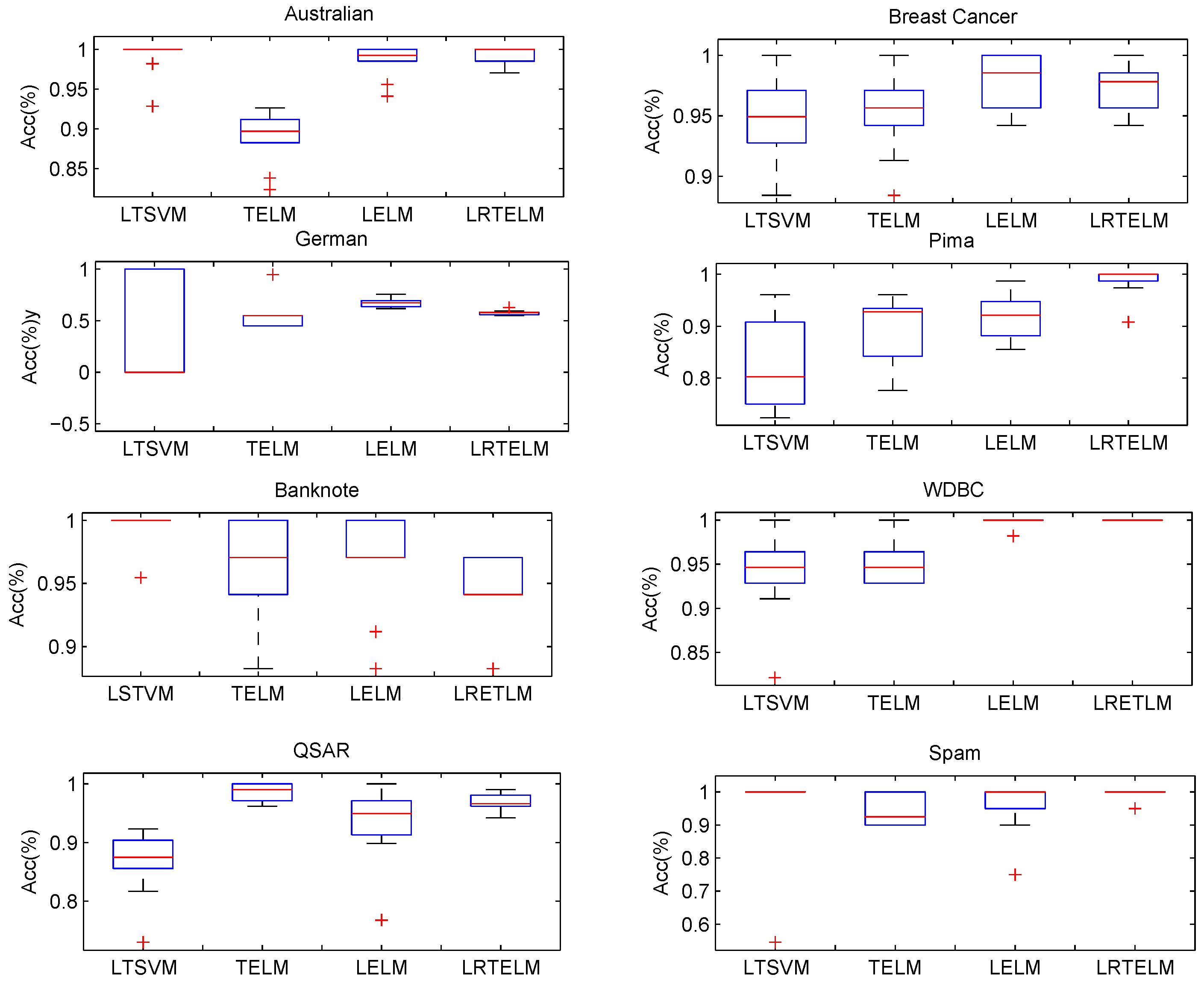
In order to statistically validate the performance of the proposed LRTELM, eight UCI datasets were selected and a series of experiments were conducted. The results of all experiments based on the optimal parameters are presented as box plots in Figure 2. Figure 2 shows the ACC box plots for LSVM, LTSVM, LELM, TELM, and LRTELM on the eight UCI datasets. The x-axis shows the different classifiers, including LSVM, LTSVM, LELM, TELM, and LRTELM, while the y-axis shows the ACC for all UCI datasets. From Figure 2, it can be seen that LRTELM has better classification accuracy than the other algorithms on most of the datasets.

5.2.3. Statistical Analysis

In this section, in order to analyse the significant differences between the seven algorithms on the ten UCI datasets, we employed the well-known Friedman test [43]. This test is known to be a simple, safe, and robust non-parametric test where the null hypothesis of the test is that all algorithms have the same performance. If the null hypothesis is rejected, a post hoc Nemeny test can be performed [43]. The average ranks of the five algorithms on all used datasets are shown in Table 3 and Table 4, respectively.

To begin with, we can calculate the Friedman statistic variable using the following formulation:

$${\chi }_F^2=\frac{12N}{k(k+1)}[\sum _j{R}_j^2-\frac{k{(k+1)}^2}{4}]=39.84$$

where k is number of algorithms, N is number of UCI datasets, and $R_j$ is the average rank of the jth algorithm on the employed datasets; note that $k=7$ and $N=10$ in this paper. Furthermore, according to the ${\chi }_F^2$-distribution with $(k-1)$ degrees of freedom, we have:

$$F_F=\frac{(N-1){\chi }_F^2}{N(k-1)-{\chi }_F^2}=19.36$$

where $F_F((k-1),(k-1)(N-1))$ obeys F-distribution with $(k-1)$ and $(k-1)(N-1)$ degrees of freedom. In addition, for $\alpha =0.05$ we can obtain $F_{\alpha }=(4,16)=3.01$. Obviously, the value of $F_F>F_{\alpha }$; thus, the null hypothesis can be rejected.

Next, we further compare the seven algorithms in pairs using the Nemenyi post hoc test. The difference in performance between the two algorithms is significant when the average rank difference between the two algorithms is larger than the critical value, otherwise the difference is not significant. By dividing the Studentized range statistic by $\sqrt{2}$, we obtain $q_{\alpha =0.05}=2.728$. Therefore, we can calculate the critical difference (CD) using the following formulation:

$$CD=q_{\alpha =0.05}\sqrt{\frac{k(k+1)}{6N}}=2.728\times \sqrt{\frac{5(5+1)}{6\times 5}}=2.728$$

Thus, if the average rank of the two algorithms differs by at least $CD$, their performance is significantly different. From Table 3, we can conclude that the proposed LRTELM differs from the other four algorithms as follows:

$$D(LSVM-LRTELM)=4-1=3>2.728$$

$$D(LTSVM-LRTELM)=5-1=4>2.728$$

$$D(TELM-LRTELM)=2.8-1=1.8<2.728$$

$$D(LELM-LRTELM)=2.2-1=1.2<2.728$$

where $D(A-B)$ denotes the difference between two algorithms, A and B. We can then conclude that the proposed LRTELM performs significantly better than LSVM and LTSVM on the NIR spectral dataset, while there is no significant difference between LRTELM, TELM, and LELM. Similarly, on the UCI dataset, it can be seen that the proposed LRTELM performs significantly better than LSVM, while there is no significant difference between LRTELM, LTSVM, TELM, and LELM according to the mean rank and correlation values reported in Table 4.

5.3. Semi-Supervised Learning Results

5.3.1. Experimental Results on Artificial Datasets

To verify the effect of manifold regularization on model performance, in this section we use the two artificial datasets [44,45] shown in Figure 3 to investigate the performance of our proposed Lap-LRTELM. Each dataset contains 200 samples with two randomly selected labeled samples and 98 unlabeled samples for every class.

Here, we analyze the effects of the $C_3$ parameters on the performance of our proposed Lap-LRTELM; $C_3$ is used to control the weight of ${\parallel f\parallel }_{\mathcal{M}}^2$. For the parameter $C_3$, the optimal parameters are $C_1=2^3$, $C_2=2^2$, and $L=200$, $N=7$, and we select different $C_3$ from the set $\{2^{-3},2^{-2},2^{-1},2^0,2^1,2^2,2^3\}$ in order to observe the impact of $C_3$ on the performance of the proposed Lap-LRTELM. It is easy to see from Figure 4 that the shape of the curve grows in the beginning and then falls when $n>2$. This means that ${\parallel f\parallel }_{\mathcal{M}}^2$ can improve the performance of Lap-LRTELM with $C_3$.

Table 5. Performance comparison of the SS-ELM, Lap-TELM, LRTELM, and Lap-LRTELM on the two lines and two moon datasets.

	LRTELM	SS-ELM	Lap-TELM	Lap-LRTELM
Datasets	ACC (%)	ACC (%)	ACC (%)	ACC (%)
	Times (s)	Times (s)	Times (s)	Times (s)
Two lines	87.12	92.25	94.51	$\mathbf{95.39}$
	2.232	3.154	2.105	1.396
Two moons	92.35	95.54	97.33	$\mathbf{98.26}$
	3.437	5.205	3.285	3.116

shows the classification accuracy of TELM, LRTELM, Lap-TELM, and Lap-LRTELM on the artificial datasets. According to the results shown in Table 5, it is obvious that when the tagged data are relatively small, the learning efficiency of Lap-LRTELM is better than the other three algorithms.

From the above experimental analysis of two artificial datasets, we can conclude that the performance of the proposed Lap-TELM is indeed improved by incorporating manifold regularisation. Intuitively, manifold regularisation can help the algorithm to seek a more reasonable classifier.

5.3.2. Experimental Results on UCI Datasets

In this section, to evaluate the effectiveness of Lap-LRTELM, we conduct experiments with different fractions of labeled samples, i.e., $10\%$ and $30\%$. In our experiments, the SS-ELM, Lap-LELM, Lap-TELM, and Lap-LRTELM were used to construct data adjacency graphs using K-nearest neighbors. All of experimental results are presented in

Table 6. Performance comparison of Lap-LELM, LRTELM, SS-ELM, Lap-TELM, and Lap-LRTELM on UCI datasets.

Datasets	Percentage	Lap-LELM	LRTELM	SS-ELM	Lap-TELM	Lap-LRTELM
	of Labeled	ACC (%)	ACC (%)	ACC (%)	ACC (%)	ACC (%)
	Samples	(${\mathit{C}}^{*}$, ${\mathit{L}}^{*}$, ${\mathit{N}}^{*}$)	(${\mathit{C}}^{*}$, ${\mathit{L}}^{*}$)	(${\mathit{\lambda }}^{*}$, ${\mathit{L}}^{*}$, ${\mathit{N}}^{*}$)	(${\mathit{C}}^{*}$, ${\mathit{L}}^{*}$, ${\mathit{N}}^{*}$)	(${\mathit{C}}^{*}$, ${\mathit{L}}^{*}$, ${\mathit{N}}^{*}$)
Diabetic	10%	58.78	59.65	59.74	59.53	$\mathbf{59.93}$
($1151\times 19$)		($2^2$, 1000, 7)	($2^3$, 1000)	($2^2$, 1000, 7)	($2^1$, 500, 7)	($2^3$, 1000, 7)
	30%	59.86	60.14	60.25	60.21	$\mathbf{61.08}$
		($2^2$, 1000, 5)	(${10}^3$, 1000)	($2^1$, 1000, 7)	($2^3$, 1000, 7)	($2^3$, 1000, 5)
Australian	10%	85.45	$\mathbf{86.89}$	84.82	84.55	86.37
($690\times 14$)		($2^0$, 500, 3)	($2^1$, 500)	($2^{-2}$, 500, 3)	($2^3$, 500, 3)	($2^2$, 1000, 3)
	30%	86.27	$\mathbf{87.36}$	85.64	85.53	86.73
		($2^2$, 500, 3)	($2^1$, 500)	($2^2$, 500, 3)	($2^3$, 500, 3)	($2^3$, 1000, 3)
Banknote	10%	83.34	83.56	84.53	84.67	$\mathbf{84.97}$
($1372\times 4$)		($2^1$, 1000, 5)	($2^3$, 500)	($2^1$, 500, 5)	($2^3$, 1000, 5)	($2^2$, 1000, 5)
	30%	87.28	86.75	88.79	88.58	$\mathbf{89.38}$
		($2^2$, 1000, 5)	($2^2$, 500)	($2^3$, 1000, 5)	($2^2$, 1000, 5)	($2^2$, 1000, 5)
Breast Cancer	10%	96.63	95.13	94.23	95.65	$\mathbf{97.24}$
($699\times 9$)		($2^2$, 500, 3)	($2^0$, 500)	($2^1$, 500, 3)	($2^0$, 500, 3)	($2^3$, 1000, 3)
	30%	97.38	96.45	96.74	96.86	$\mathbf{98.29}$
		($2^0$, 500, 3)	($2^2$, 500)	($2^1$, 500, 3)	($2^1$, 500, 3)	($2^3$, 1000, 3)
WDBC	10%	$\mathbf{93.83}$	92.33	93.43	93.57	93.66
($569\times 30$)		($2^3$, 500, 3)	($2^2$, 500)	($2^3$, 500, 3)	($2^1$, 500, 3)	($2^3$, 500, 3)
	30%	$\mathbf{94.41}$	93.13	94.11	94.14	94.27
		($2^3$, 500, 3)	($2^2$, 500)	($2^3$, 500, 3)	($2^3$, 500, 3)	($2^2$, 500, 3)
German	10%	72.96	71.13	76.39	76.89	$\mathbf{77.66}$
($1000\times 24$)		($2^4$, 1000, 7)	($2^0$, 500)	($2^2$, 500, 7)	($2^0$, 500, 3)	($2^2$, 500, 5)
	30%	76.11	78.93	78.81	78.91	$\mathbf{79.11}$
		($2^4$, 1000, 7)	($2^0$, 500)	($2^{-1}$, 500, 7)	($2^1$, 500, 3)	($2^1$, 500, 5)
Pima	10%	86.81	81.79	81.18	81.65	$\mathbf{89.64}$
($768\times 8$)		($2^2$, 500, 3)	($2^0$, 500)	($2^2$, 500, 3)	($2^3$, 500, 3)	($2^3$, 1000, 3)
	30%	88.64	83.55	83.38	83.75	$\mathbf{93.03}$
		($2^1$, 500, 5)	($2^0$, 500)	($2^{-1}$, 500, 3)	($2^1$, 500, 5)	($2^2$, 1000, 5)
QSAR	10%	85.75	85.14	86.54	86.24	$\mathbf{87.54}$
($1055\times 41$)		($2^3$, 1000, 9)	($2^2$, 1000)	($2^3$, 1000, 9)	($2^1$, 1000, 5)	($2^2$, 1000, 3)
	30%	89.58	86.25	89.66	89.46	$\mathbf{91.21}$
		($2^2$, 1000, 9)	($2^2$, 1000)	($2^0$, 1000, 9)	($2^2$, 1000, 5)	($2^2$, 1000, 3)
Spam	10%	90.27	89.63	89.47	89.83	$\mathbf{90.89}$
($4601\times 57$)		($2^2$, 3000, 9)	($2^1$, 3000)	($2^3$, 3000, 9)	($2^{-1}$, 3000, 9)	($2^0$, 3000, 9)
	30%	92.76	90.85	90.31	90.78	$\mathbf{92.37}$
		($2^1$, 5000, 9)	($2^3$, 5000)	($2^2$, 5000, 9)	($2^{-1}$, 5000, 9)	($2^2$, 5000, 9)
Avg.ACC	10%	83.65	82.81	83.37	83.62	$\mathbf{85.32}$
Avg.ACC	30%	85.81	84.82	85.30	85.36	$\mathbf{87.28}$
Avg.rank	10%	3.11	3.78	3.56	3.33	$\mathbf{1.22}$
Avg.rank	30%	3	3.78	3.56	3.44	$\mathbf{1.22}$

.

From Table 6, it can be seen that the performance of all the algorithms improves as the number of labelled samples increases. Furthermore, we find that the proposed Lap-LRTELM outperforms the other algorithms in most cases, regardless of the size of the labelled samples. Furthermore, the generalisation performance of the proposed Lap-LRTELM outperforms the other relevant ELM-based algorithms on all datasets.

The analysis of the above experimental results shows that the proposed Lap-LRTELM improves the classification performance of the LRTELM by using flow regularisation. Intuitively, a reasonable classifier can be built using manifold regularisation.

5.3.3. Experimental Results on Image Datasets

To further verify the performance of Lap-LRTELM, we performed experiments on the G50C (http://people.cs.uchicago.edu/vikass/manifoldregularization.html) (accessed on 22 March 2021), COIL20(B) (http://www.cs.columbia.edu/CAVE/software/softlib/coil-20.php) (accessed on 22 March 2021), USPST(B) (http://www.cad.zju.edu.cn/home/dengcai/Data/MLData.html) (accessed on 22 March 2021), and MNIST(B) (http://yann.lecun.com/exdb/mnist/) (accessed on 22 March 2021) datasets.

To rationally demonstrate the semi-supervised approach involved, we utilised the equivalent experimental setup reported by Melacci and Belkin [24]. Concretely, we employed a four-fold cross-validation approach for each image dataset, with one fold as the test set (denoted by $\mathcal{T}$) and the remaining folds as the training set. The training set was divided into labelled data ($\mathcal{L}$), unlabelled data ($\mathcal{U}$), and validation data ($\mathcal{V}$). Here, this random folding was repeated three times, producing a total of twelve divisions. Detailed information on the datasets is summarized in

Table 7. Description of the datasets.

Datasets	$\left|\mathcal{L}\right|$	$\left|\mathcal{U}\right|$	$\left|\mathcal{V}\right|$	$\left|\mathcal{T}\right|$
G50C	50	313	50	137
COIL20(B)	40	1000	50	360
USPST(B)	50	1409	50	498
MNIST(B)	200	1100	200	500

.

The performance of these algorithms on the USPST(B), COIL20(B), G50C, and MNIST(B) datasets was evaluated in our experiments using ACC ± S (classification accuracy ± standard deviation); the experimental results are shown in

Table 8. Performance comparison of LRTELM, SS-ELM, Lap-LELM, Lap-TELM, and Lap-LRTELM.

Datasets	Subset	LRTELM	SS-ELM	Lap-LELM	Lap-TELM	Lap-LRTELM
		ACC ± S (%)	ACC ± S (%)	ACC ± S (%)	ACC ± S (%)	ACC ± S (%)
COIL20(B)	$\mathcal{U}$	86.47 ± 1.78	86.38 ± 2.12	86.79 ± 2.31	89.08 ± 2.64	$\mathbf{90.25}\pm \mathbf{1.54}$
	$\mathcal{V}$	89.28 ± 2.32	88.60 ± 1.96	88.81 ± 2.64	91.13 ± 3.42	$\mathbf{91.29}\pm \mathbf{2.88}$
	$\mathcal{T}$	86.37 ± 1.22	86.47 ± 2.68	86.61 ± 2.63	89.44 ± 4.00	$\mathbf{91.58}\pm \mathbf{1.54}$
USPST(B)	$\mathcal{U}$	89.67 ± 3.74	90.78 ± 3.49	91.56 ± 2.72	91.83 ± 0.40	$\mathbf{92.66}\pm \mathbf{1.38}$
	$\mathcal{V}$	91.25 ± 2.56	91.58 ± 2.34	91.75 ± 4.38	91.34 ± 0.94	$\mathbf{93.42}\pm \mathbf{1.52}$
	$\mathcal{T}$	89.53 ± 2.59	90.12 ± 2.66	90.47 ± 2.76	90.74 ± 0.62	$\mathbf{92.895}\pm \mathbf{1.53}$
G50C	$\mathcal{U}$	91.18 ± 3.26	93.85 ± 1.57	88.67 ± 5.39	91.77 ± 2.53	$\mathbf{93.87}\pm \mathbf{2.26}$
	$\mathcal{V}$	92.33 ± 3.06	92.35 ± 1.53	85.83 ± 4.78	95.17 ± 3.24	$\mathbf{94.45}\pm \mathbf{3.34}$
	$\mathcal{T}$	91.27 ± 3.76	93.49 ± 1.45	82.54 ± 2.65	92.27 ± 3.06	$\mathbf{94.59}\pm \mathbf{2.56}$
MNIST(B)	$\mathcal{U}$	85.47 ± 2.76	89.33 ± 1.29	89.78 ± 1.77	90.36 ± 1.13	$\mathbf{91.58}\pm \mathbf{1.63}$
	$\mathcal{V}$	87.66 ± 3.62	90.42 ± 2.22	91.56 ± 1.86	92.04 ± 1.80	$\mathbf{92.69}\pm \mathbf{1.78}$
	$\mathcal{T}$	85.49 ± 1.39	87.05 ± 1.49	89.64 ± 1.58	89.88 ± 1.34	$\mathbf{91.32}\pm \mathbf{1.46}$

.

As can be seen from Table 8, Lap-LRTELM outperforms the other five algorithms in terms of classification accuracy on all the datasets involved. Compared with LRTELM, the proposed Lap-LRTELM can effectively utilise unlabelled samples to produce better performance. The experimental results show that by taking streamwise regularisation into account, the proposed Lap-LRTELM can achieve better performance compared to considering only one part.

To analyse the influences of labelled and unlabelled samples on the performance of the relevant semi-supervised methods, we conducted a further series of experiments on COIL20(B), USPST(B), and G50C. The results of all experiments are shown in Figure 5 and Figure 6.

Figure 5 shows the classification accuracy of SS-ELM, Lap-TELM, Lap-LELM, and Lap-RTELM for different labelled samples on COIL20(B), USPST(B), G50C, and MNIST(B). As can be seen from the following Figure 5, in most cases Lap-RTELM achieves the best results relative to the other three algorithms. The classification accuracy of all algorithms improves substantially as the number of labelled samples increases. 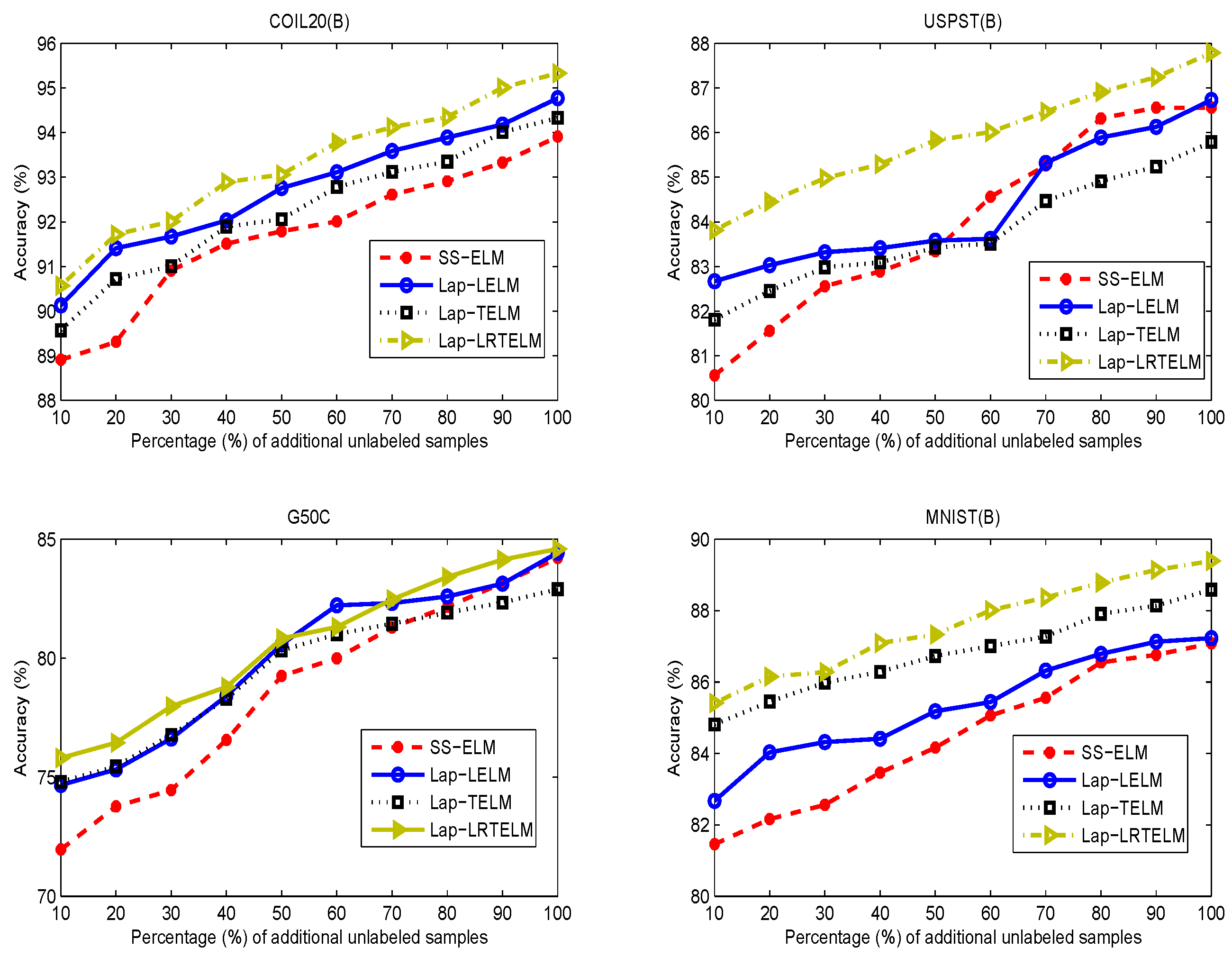Figure 6 shows the performance of the four semi-supervised algorithms for different numbers of unlabelled samples. Using the same experimental scheme as in [29], we add unlabelled samples to the unlabelled set ($\mathcal{U}$) in 10% increments, while the labelled set ($\mathcal{L}$), test set ($\mathcal{T}$), and validation set ($\mathcal{V}$) remain unchanged. From Figure 6, it is easy to observe that classification accuracy improves when unlabelled samples are added to the unlabelled set ($\mathcal{U}$). Even without any labelled ones, Lap-LRTELM performs better than SS-ELM, Lap-TELM and Lap-LELM. This phenomenon is consistent with Belkin et al. [24] in that stream regularization is effective for purely supervised learning.

5.3.4. Statistical Analysis

In this section, we use the famous Friedman test with the corresponding post hoc test [43] to analyze and compare algorithms’ performance on UCI datasets. The average ranking of the five algorithms on all datasets used is shown in Table 6. First, we compare the performance of the five algorithms on the UCI dataset, in which 10% of the sample was labelled.

To begin with, we can calculate the Friedman statistic variable using the following formulation:

$${\chi }_F^2=\frac{12N}{k(k+1)}[\sum _j{R}_j^2-\frac{k{(k+1)}^2}{4}]=10.95$$

where k is number of algorithms, N is the number of UCI datasets, and $R_j$ is the average rank of the jth algorithm on the employed datasets; note that $k=7$ and $N=10$ in this paper. Furthermore, according to the ${\chi }_F^2$-distribution with $(k-1)$ degrees of freedom, we have:

$$F_F=\frac{(N-1){\chi }_F^2}{N(k-1)-{\chi }_F^2}=3.497$$

where $F_F((k-1),(k-1)(N-1))$ obeys F-distribution with $(k-1)$ and $(k-1)(N-1)$ degrees of freedom. In addition, for $\alpha =0.05$ we can obtain $F_{\alpha }=(4,32)=2.69$. Obviously, the value of $F_F>F_{\alpha }$; thus, the null hypothesis can be rejected.

Furthermore, we compared the seven algorithms in pairs using the Nemenyi post hoc test. The difference in performance between the two algorithms is significant when the average rank difference between the two algorithms is larger than the critical value; otherwise, the difference is not significant. By dividing the Studentized range statistic by $\sqrt{2}$, we obtain $q_{\alpha =0.05}=2.728$. Therefore, we can calculate the critical difference (CD) using the following formulation:

$$CD=q_{\alpha =0.05}\sqrt{\frac{k(k+1)}{6N}}=2.728\times \sqrt{\frac{5(5+1)}{6\times 9}}=2.03$$

Thus, if the average ranks of two algorithms differ by at least $CD$, their performance is significantly different. From Table 6, we can derive the differences between the proposed Lap-LRTELM and other four algorithms as follows:

$$D(Lap-LELM-Lap-LRTELM)=1.89<2.03$$

$$D(LRTELM-Lap-LRTELM)=2.56>2.03$$

$$D(SS-ELM-Lap-LRTELM)=2.34>2.03$$

$$D(Lap-TELM-Lap-LRTELM)=2.11>2.03$$

In summary, the proposed Lap-LRTELM performs significantly better than LRTELM, SS-ELM, and Lap-TELM, and there is no significant difference between Lap-LRTELM and Lap-LELM on UCI datasets with 10% labeled samples. Similarly, on UCI datasets with 30% labeled samples, we can obtain the same conclusions based on the average ranks and relevant values reported in Table 6.

6. Conclusions

In this paper, we first propose the Lagrangian Regularized Twin Extreme Learning Machine algorithm (LRTELM). We then extend LRTELM to semi-supervised learning by introducing manifold regularisation to obtain a new semi-supervised learning framework, the Lagrangian Regularised Twin Extreme Learning Machine (Lap-LRTELM). Lap-LRTELM can effectively use geometric information embedded in the marginal distribution of unlabelled samples to construct a more reasonable classifier. A significant advantage of the proposed LRTELM and Lap-LRTELM is the implementation of the principle of SRM by adding regularization terms to the objective function. Another advantage of the proposed LRTELM and Lap-LRTELM is that only two simple linear equations need to be solved to avoid solving a pair of QPPs like TELM. Compared to existing supervised and semi-supervised ELM algorithms, the proposed LRTELM and Lap-LRTELM maintain almost all of the advantages of ELM, such as significant training efficiency for binary classification problems. These two ELM extensions for supervised and semi-supervised learning are expected to significantly extend the applicability of ELM and provide new insights into extreme learning paradigms. Experimental results on multiple datasets show that our LRTELM and Lap-LRTELM are highly effective compared to other methods.

We anticipate that ways of incorporating our methods into the multi-class classification, regression, and robust problems will be topics addressed in our future work.

References

1. Huang, G.B.; Zhu, Q.Y.; Siew, C.K. Extreme learning machine: Theory and applications. Neurocomputing 2006, 70, 489–501. [Google Scholar] [CrossRef]
2. Huang, G.; Huang, G.B.; Song, S.H.; You, K.Y. Trends in extreme learning machines: A review. Neural Netw. 2015, 61, 32–48. [Google Scholar] [CrossRef]
3. Cortes, C.; Vapnik, V. Support-Vector networks. Mach. Learn. 1995, 20, 273–297. [Google Scholar] [CrossRef]
4. Wang, G.; Zhao, Y.; Wang, D. A protein secondary structure prediction frame-work based on the extreme learning machine. Neurocomputing 2008, 72, 262–268. [Google Scholar] [CrossRef]
5. Lan, Y.; Soh, Y.C.; Huang, G.B. Extreme Learning Machine based bacterial protein subcellular localization prediction. In Proceedings of the IEEE International Joint Conference on Neural Networks, IJCNN, Hong Kong, China, 1–8 June 2008; pp. 1859–1863. [Google Scholar]
6. Mohammed, A.A.; Minhas, R.; Jonathan, Q.M.; Sid-Ahmed, M.A. Human face recognition based on multidimensional PCA and extreme learning machine. Pattern Recognit. 2011, 44, 2588–2597. [Google Scholar] [CrossRef]
7. Nizar, A.H.; Dong, Z.Y.; Wang, Y. Power utility nontechnical loss analysis with extreme learning machine method. IEEE Trans. Power Syst. 2008, 23, 946–955. [Google Scholar] [CrossRef]
8. Decherchi, S.; Gastaldo, P.; Dahiya, R.S.; Valle, M.; Zunino, R. Tactile data classification of contact materials using computational intelligence. IEEE Trans. Robot 2011, 27, 635–639. [Google Scholar] [CrossRef]
9. Choudhary, R.; Shukla, S. Reduced-Kernel Weighted Extreme Learning Machine Using Universum Data in Feature Space (RKWELM-UFS) to Handle Binary Class Imbalanced Dataset Classification. Symmetry 2022, 14, 379. [Google Scholar] [CrossRef]
10. Owolabi, T.O.; Abd Rahman, M.A. Prediction of band gap energy of doped graphitic carbon nitride using genetic algorithm-based support vector regression and extreme learning machine. Symmetry 2021, 13, 411. [Google Scholar] [CrossRef]
11. Huang, G.B.; Ding, X.J.; Zhou, H.M. Optimization method based extreme learning machine for classification. Neurocomputing 2010, 74, 155–163. [Google Scholar] [CrossRef]
12. Yang, L.; Zhang, S. A smooth extreme learning machine framework. J. Intell. Fuzzy Syst. 2017, 33, 3373–3381. [Google Scholar] [CrossRef]
13. Yang, L.; Zhang, S. A sparse extreme learning machine framework by continuous optimization algorithms and its application in pattern recognition. Eng. Appl. Artif. Intell. 2016, 53, 176–189. [Google Scholar] [CrossRef]
14. Huang, G.B.; Zhou, H.; Ding, X.; Zhang, R. Extreme learning machine for regression and multiclass classification. IEEE Trans. Syst. Man Cybern. Part B Cybern. 2012, 42, 513–529. [Google Scholar] [CrossRef] [PubMed] [Green Version]
15. Balasundaram, S.; Tanveer, M. On lagrangian twin support vector regression. Neural Comput. Appl. 2013, 22, 257–267. [Google Scholar] [CrossRef]
16. Ma, J.; Wen, Y.; Yang, L. Lagrangian supervised and semi-supervised extreme learning machine. Appl. Intell. 2019, 49, 303–318. [Google Scholar] [CrossRef]
17. Jayadeva; Khemchandani, R.; Chandra, S. Twin support vector machines for pattern classification. IEEE Trans. Pattern Anal. Mach. Intell. 2007, 29, 905. [Google Scholar] [CrossRef]
18. Peng, X. A ν-twin support vector machine (ν-TSVM) classifier and its geometric algorithms. Inf. Sci. 2010, 180, 3863–3875. [Google Scholar] [CrossRef]
19. Shao, Y.H.; Zhang, C.H.; Wang, X.B.; Deng, N.Y. Improvements on twin support vector machines. IEEE Trans. Neural Netw. 2011, 22, 962–968. [Google Scholar] [CrossRef]
20. Qi, Z.; Tian, Y.; Shi, Y. Laplacian twin support vector machine for semi-supervised classification. Neural Netw. 2012, 35, 46–53. [Google Scholar] [CrossRef]
21. Qi, Z.; Tian, Y.; Shi, Y. Robust twin support vector machine for pattern classification. Pattern Recognit. 2013, 46, 305–316. [Google Scholar] [CrossRef]
22. Shao, Y.H.; Hua, X.Y.; Liu, L.M.; Yang, Z.M.; Deng, N.Y. Combined outputs framework for twin support vector machines. Appl. Intell. 2015, 43, 424–438. [Google Scholar] [CrossRef]
23. Mangasarian, O.L.; Musicant, D.R. Lagrangian support vector machines. J. Mach. Learn. Res. 2001, 1, 161–177. [Google Scholar]
24. Balasundaram, S.; Kapil, N. Application of Lagrangian Twin Support Vector Machines for Classification. In Proceedings of the Second International Conference on Machine Learning & Computing, Washington, DC, USA, 27–29 October 2010. [Google Scholar]
25. Shao, Y.H.; Chen, W.J.; Zhang, J.J.; Wang, Z.; Deng, N.Y. An efficient weighted lagrangian twin support vector machine for imbalanced data classification. Pattern Recognit. 2014, 47, 3158–3167. [Google Scholar] [CrossRef]
26. Balasundaram, S.; Gupta, D.; Prasad, S.C. A new approach for training lagrangian twin support vector machine via unconstrained convex minimization. Appl. Intell. 2016, 46, 124–134. [Google Scholar] [CrossRef]
27. Balasundaram, S.; Gupta, D. On implicit lagrangian twin support vector regression by newton method. Int. J. Comput. Intell. Syst. 2014, 7, 50–64. [Google Scholar] [CrossRef]
28. Tanveer, M.; Shubham, K. A regularization on lagrangian twin support vector regression. Int. J. Mach. Learn. Cybern. 2017, 8, 807–821. [Google Scholar] [CrossRef]
29. Balasundaram, S.; Gupta, D. Training lagrangian twin support vector regression via unconstrained convex minimization. Knowl.-Based Syst. 2014, 59, 85–96. [Google Scholar] [CrossRef]
30. Tanveer, M.; Shubham, K.; Aldhaifallah, M.; Nisar, K.S. An efficient implicit regularized lagrangian twin support vector regression. Appl. Intell. 2016, 44, 831–848. [Google Scholar] [CrossRef]
31. Belkin, M.; Niyogi, P.; Sindhwani, V. Manifold Regularization: A Geometric Framework for Learning from Labeled and Unlabeled Examples. J. Mach. Learn. Res. 2006, 7, 11. [Google Scholar]
32. Chapelle, O.; Sindhwani, V.; Keerthi, S.S. Optimization techniques for semi-supervised support vector machines. J. Mach. Learn. Res. 2008, 9, 203–233. [Google Scholar]
33. Melacci, S.; Belkin, M. Laplacian support vector machines trained in the primal. J. Mach. Learn. Res. 2009, 12, 1149–1184. [Google Scholar]
34. Zhu, X. Semi-Supervised Learning Literature Survey. 2005. Available online: https://pages.cs.wisc.edu/~jerryzhu/pub/ssl_survey.pdf (accessed on 20 May 2022).
35. Huang, G.; Song, S.; Gupta, J.N.D.; Wu, C. Semi-Supervised and unsupervised extreme learning machines. IEEE Trans. Cybern. 2014, 44, 2405. [Google Scholar] [CrossRef] [PubMed]
36. Liu, B.; Xia, S.X.; Meng, F.R.; Zhou, Y. Manifold regularized extreme learning machine. Neural Comput. Appl. 2016, 27, 255–269. [Google Scholar] [CrossRef]
37. Li, S.; Song, S.; Wan, Y. Laplacian Twin Extreme Learning Machine for Semi-supervised Classificatio. Neurocomputing 2018, 321, 17–27. [Google Scholar] [CrossRef]
38. Schölkopf, B.; Smola, A. Learning with Kernels: Support Vector Machines, Regularization, Optimization, and Beyond; MIT Press: Cambridge, MA, USA, 2001. [Google Scholar]
39. Bertsekas, D.P. Nonlinear programming. J. Oper. Res. Soc. 1997, 48, 334. [Google Scholar] [CrossRef]
40. Wan, Y.; Song, S.; Huang, G.; Li, S. Twin extreme learning machines for pattern classification. Neurocomputing 2017, 260, 235–244. [Google Scholar] [CrossRef]
41. Gao, X.; Lu, T.; Liu, P.; Lu, Q. A soil moisture classification model based on SVM used in agricultural WSN. In Proceedings of the IEEE Joint International Information Technology & Artificial Intelligence Conference, Chongqing, China, 20–21 December 2015. [Google Scholar]
42. Pierna, J.F.; Lecler, B.; Conzen, J.P.; Niemoeller, A.; Baeten, V.; Dardenne, P. Comparison of various chemometric approaches for large near infrared spectroscopic data of feed and feed products. Anal. Chim. Acta 2011, 705, 30–34. [Google Scholar] [CrossRef]
43. Demišar, J.; Schuurmans, D. Statistical comparisons of classifiers over multiple data sets. J. Mach. Learn. Res. 2006, 7, 1–30. [Google Scholar]
44. Chen, W.J.; Shao, Y.H.; Hong, N. Laplacian smooth twin support vector machine for semi-supervised classification. Int. J. Mach. Learn. Cybern. 2014, 5, 459–468. [Google Scholar] [CrossRef]
45. Pei, H.; Wang, K.; Lin, Q.; Zhong, P. Robust semi-supervised extreme learning machine. Knowl.-Based Syst. 2018, 159, 203–220. [Google Scholar] [CrossRef]
Figure 1. The learning times of the LSVM, LTSVM, TELM, LELM, and LRTELM on near-infrared spectral datasets.
Symmetry 14 01186 g001
Figure 2. ACC performance comparison of LSTVM, TELM, LELM, and LRTELM on eight UCI datasets.
Symmetry 14 01186 g002
Figure 3. Distribution of the two lines and two moon datasets: (a) two lines dataset and (b) two moon dataset.
Symmetry 14 01186 g003
Figure 4. Learning results of Lap-LRTELM on the two lines and two moon datasets with different values of parameter C 3 ( C 3 = 2 n ).
Symmetry 14 01186 g004
Figure 5. Comparing the classification accuracy of SS-ELM, Lap-LELM, Lap-TELM, and Lap-LRTELM on COIL20(B), USPST(B), G50C, and MNIST(B) datasets with different numbers of labeled samples.
Symmetry 14 01186 g005
Figure 6. Comparing the classification accuracy of SS-ELM, Lap-LELM, Lap-TELM, and Lap-LRTELM on COIL20(B), USPST(B), G50C, and MNIST(B) datasets with different numbers of unlabeled samples.
Symmetry 14 01186 g006