Learning Coupled Oscillators System with Reservoir Computing

Abstract

In this paper, we reconstruct the dynamic behavior of the ring-coupled Lorenz oscillators system by reservoir computing. Although the reconstruction of various complex chaotic attractors has been well studied by using various neural networks, little attention has been paid to whether the spatio-temporal structure of some special attractors can be maintained in long-term prediction. Reservoir computing has been shown to be effective for model-free prediction, so we want to investigate whether reservoir computing can restore the rotational symmetry of the original ring-coupled Lorenz system. We find that although the state prediction of the trained reservoir computer will gradually deviate from the actual trajectory of the original system, the associated spatio-temporal structure is maintained in the process of reconstruction. Specifically, we show that the rotational symmetric structure of periodic rotating waves, quasi-periodic torus, and chaotic rotating waves is well maintained.

1. Introduction

The synchronization of chaotic systems is a basic problem of nonlinear science, which has attracted the extensive attention of scientists [1,2,3,4,5,6,7,8]. For example, Pecora and Carroll in [1] found that synchronization can be achieved by connecting two chaotic systems with a common signal. Fujisaka and Yamada in [5,6,7,8] showed that synchronization could be achieved in symmetrically coupled identical chaotic systems. In general, previous studies of chaos synchronization rely on the fact that the equations of chaotic systems are known. However, it is impossible to deal with real chaotic systems using limited observational data [9].

Recently, some model-free prediction methods have been proposed for the synchronization of chaotic systems using reservoir computing methods [10,11,12,13]. The state evolution of chaotic systems is predicted by RC [14,15,16,17,18,19]. The idea and principle of using reservoir computing for model-free systems are first proposed about two decades ago [10,19]. Especially it can be driven by the data to reconstruct the original system. Such as, Chen et al. in [13] showed that reservoir computing can learn the topological characteristics of dynamical systems. Lu et al. in [20] reported that reservoir computing learns similar attractors from the original system under an appropriate choice of parameters. Zhang et al. in [21] showed that reservoir computing could learn Hamiltonian dynamics. They suggested that reservoir computing could reconstruct the dynamics of the original system. It is worth noting that these works mainly study a trained reservoir network from the respective dynamics, while the underlying dynamic characteristics of complex networks with multiple oscillator coupling have received little attention. Recently, the study of complex networks has always attracted the attention of scientists because of its structural complexity, especially the ring-coupled Lorenz oscillators. For example, Sánchez et al. in [22,23] studied the transition between periodic rotating waves and synchronized chaos in unidirectional coupled Lorenz oscillators ring. Wang et al. in [24] demonstrated the existence of the rotating wave by Hopf bifurcation of rotating periodic solutions in the coupled Lorenz systems. Horikawa et al. in [24] showed chaotic transient rotating waves in a ring of unidirectionally coupled bistable Lorenz systems. Therefore, it is of great significance to study the dynamic characteristics of the complex network by using the reservoir computing method. Moreover, multiple oscillator coupling systems usually have special spatio-temporal symmetries, which will be the major motivation of our research.

In this paper, we focus on studying reconstruction problems on various dynamical behaviors in unidirectional coupled Lorenz systems with the principle of synchronization and reservoir computing. The coupled network has rich complexity, and it includes stable point, periodic rotating wave, synchronous chaos, chaos rotating wave, and invariant torus in [22,23,24]. Thus, we want to know: (1) whether the above dynamic behaviors can be maintained in the process of reconstruction with reservoir computing technology and (2) whether the spatio-temporal structure investigated in [24,25,26] can preserve during the reconstruction process, especially whether the rotational symmetry in the spatio-temporal structure can be maintained in the reconstruction process, (3) whether the bifurcation point is consistent with the original system.

This paper is organized as follows: In Section 2, we briefly introduce the unidirectional coupled Lorenz systems and the studied models. We provide the application method of reservoir computation in Section 3. The numerical experiment will be reported in Section 4. Discussion and a conclusion will be provided in Section 5.

2. Description of the System

The time series comes from the following equation:

$$\{\begin{array}{l}\frac{{dx}_n}{dt}=\sigma (y_n-x_n),\hfill \\ \frac{{dy}_n}{dt}=R{x}_{n-1}-y_n-x_n{z}_n,\hfill \\ \frac{d{z}_n}{dt}=-\beta z_n+x_n{y}_n(1\le n\le N,x_0=x_N).\hfill \end{array}$$

(1)

Here, $\sigma ,R,\beta$ represent the corresponding parameters of the Lorenz system, and $x_n,y_n,z_n$ represent the dynamical state of the $nth$ oscillator. System (1) consists of a ring of n unidirectional coupled Lorenz oscillators. For further research, in this paper, we want to reconstruct the complex system with multiple oscillators coupling. Due to the complexity of the spatio-temporal structure, the system can display rich, dynamic behaviors [22,23,24], such as fixed point, synchronous chaos, quasi-periodic behavior, periodic rotating wave, or a chaotic rotating wave of high-dimensional chaos. Among them, the rotational symmetry of chaotic rotating waves and quasi-periodic and periodic rotating waves are the focus of our research. In [24], the authors used the method of rotating periodic solutions to obtain the periodic synchronous solution of the above system. Rotating periodic solutions as a generalization of periodic solutions can be expressed by equations $x(t+T)=Qx(t)$ with some orthogonal matrix $Q$ [27,28,29,30]. We will focus on the reconstruction of a ring of three unidirectional coupled Lorenz oscillators. According to the results in [29], we can find the solution of the original system in two forms of the synchronous solution by searching the matrix $Q$ that satisfies the condition of rotating periodic solution. We can find the following rotating matric $Q$ satisfying rotating periodic condition

$$Q_1=\left(\begin{array}{ccc}0& 1& 0\\ 0& 0& 1\\ 1& 0& 0\end{array}\right),Q_2=\left(\begin{array}{ccc}0& 0& 1\\ 1& 0& 0\\ 0& 1& 0\end{array}\right).$$

All the above matrices $Q_1-Q_2$ and identity matrix $I_3$ form a group ${\mathrm{\Gamma }}_1$. Moreover, all matrices $-Q_i(i=1,2)$ and $-I_3$ also satisfy the rotating periodic condition. Since the type of synchronous solution is only related to the difference of variable angle values in the eigenvalues of the matrices $Q$ and the matrices $Q$, $-Q$ provide the same type of synchronous solution, we only need the matrices in the group Γ to attain all types of synchronous solutions [26]. What is more, all the rotating matrices corresponding to the same type of synchronous solutions are similar. Thus, we can obtain all types of synchronous solutions from the conjugate classes $C_i(i=1,\dots ,m)$ of the group $\mathrm{\Gamma }$. In fact, after diagonalizing $Q$, we find that $Q$ has only two forms, which represent the complete synchronization of the oscillator and the synchronization with the same phase difference of $\frac{2\pi }{n}$, respectively. Since the system has multiple Hopf bifurcation points, it is possible for the system to produce invariant torus and even chaos [22,23,24]. Phase space reconstruction is a method of recovering and characterizing the original dynamic system from known time series. In short, it is a method of recovering the original system from time series; a typical method regards the system reconstructed in phase space as the synchronization system of the original system. In [31], Pecora and Carroll decided that combining two identical chaotic systems in a particular way was to take a signal from a component of the transmitter and send it to the receiver where the receiver was missing the part of the system. However, this missing part was retained by using the received signals. Thus, they demonstrated that by choosing the variable $x$ to drive the Lorenz system, then $y^{\prime }$ and $z^{\prime }$ subsystems will converge to $y$ and $z$ as the systems evolve together on identical trajectories. The system in [31] is expressed by Equation (2), and we can see it as the driven-response system as follows.

$$\begin{array}{c}\stackrel{.}{x}=\sigma (y-x),\\ \dot{y}=-xz+rx-y {\dot{y}}^{\prime }=-x{z}^{\prime }+rx-y^{\prime },\\ \dot{z}=xy-bz {\dot{z}}^{\prime }=x{y}^{\prime }-b{z}^{\prime }.\end{array}$$

(2)

In Equation (2), the $x-y-z$ model is the driven system, and the $x-y^{\prime }-z^{\prime }$ model is the response system. Using the variable $x$ to drive the response system and observe the relationship between the driven system and the response system.

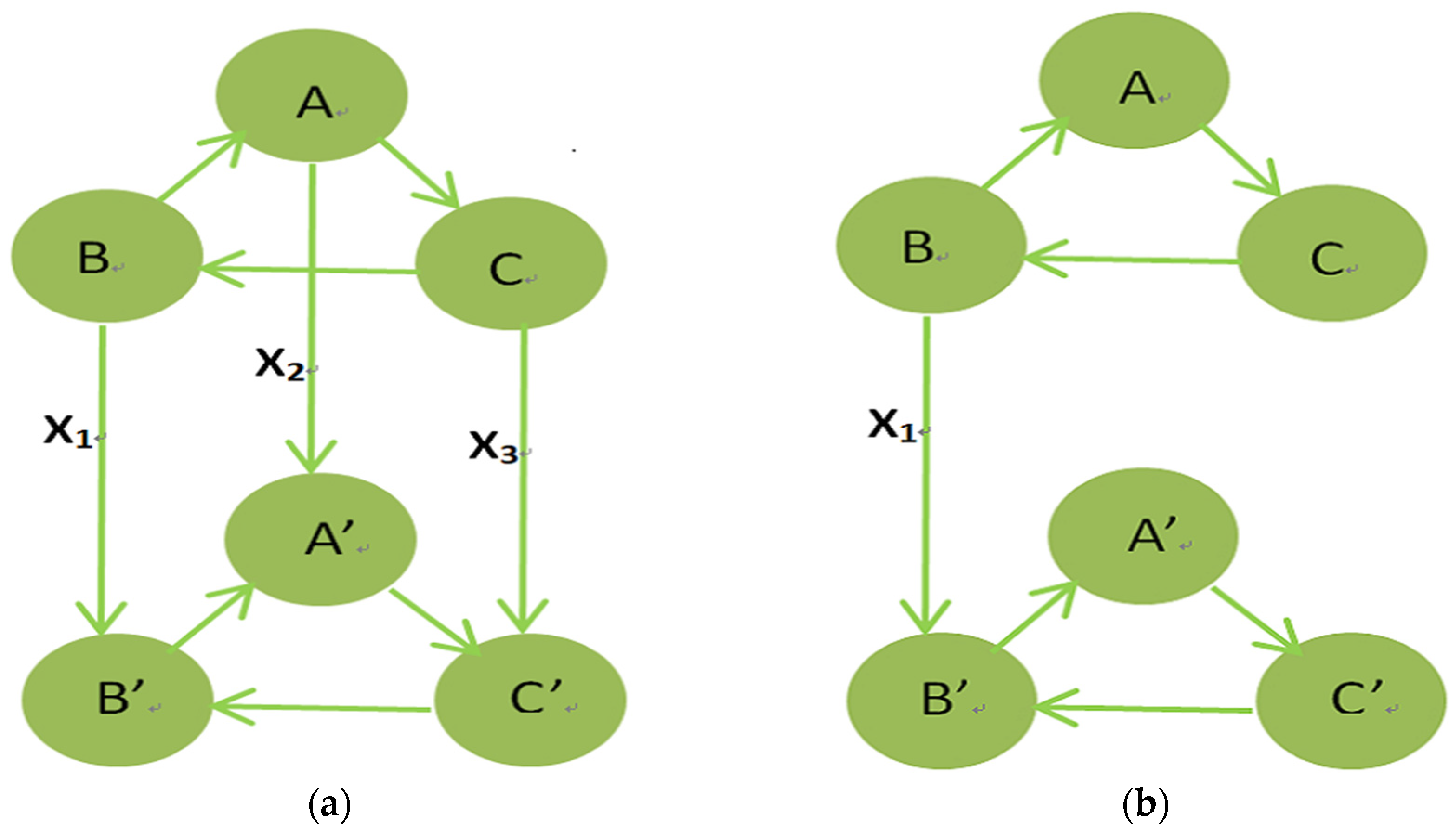
Similarly, we provide two similar drive-response systems according to Equation (2) that have three signals input and one signal input. Then, we can attain two different response systems. We will use the double-layer coupled network model to simulate two drive-response systems (see Figure 1a,b). Equation (1) is regarded as the driven system, $x_i,y_i,z_i$ are the state variable of the $ith$ oscillator of the driven system, $X_i,Y_i,Z_i$ are the state variable of the response system. Equation (3) represents the three signals driven-response system.

$$\{\begin{array}{l}\frac{d{x}_n}{dt}=\sigma (y_n-x_n),\hfill \\ \frac{d{y}_n}{dt}=R{x}_{n-1}-y_n-x_n{z}_n\hfill \\ \frac{d{z}_n}{dt}=-\beta z_n+x_n{y}_n,\hfill \end{array},\{\begin{array}{l}\frac{d{Y}_n}{dt}=R{x}_{n-1}-Y_n-x_n{Z}_n,\hfill \\ \frac{d{Z}_{\mathrm{n}}}{dt}=-\beta Z_n+x_n{Y}_n(1\le n\le N,x_0=x_N).\hfill \end{array}$$

(3)

Equation (4) represents the one signal drive-response system.

$$\{\begin{array}{l}\frac{d{x}_n}{dt}=\sigma (y_n-x_n),\hfill \\ \frac{d{y}_n}{dt}=R{x}_{n-1}-y_n-x_n{z}_n\hfill \\ \frac{d{z}_n}{dt}=-\beta z_n+x_n{y}_n,\hfill \end{array},\{\begin{array}{l}\frac{d{Y}_1}{dt}=R{X}_3-Y_1-x_1{Z}_1,\hfill \\ \frac{d{Z}_1}{dt}=-\beta Z_1+x_1{Y}_1,\hfill \\ \frac{d{X}_2}{dt}=\sigma (Y_2-X_2),\hfill \\ \frac{d{Y}_2}{dt}=R{x}_1-Y_2-X_2{Z}_2,\hfill \\ \frac{d{Z}_2}{dt}=-\beta Z_2+X_2{Y}_2,\hfill \\ \frac{d{X}_3}{dt}=\sigma (Y_3-X_3),\hfill \\ \frac{d{Y}_3}{dt}=R{X}_2-Y_3-X_3{Z}_3,\hfill \\ \frac{d{Z}_3}{dt}=-\beta Z_3+X_3{Y}_3.\hfill \end{array}$$

(4)

The synchronization between systems constitutes the theoretical basis of phase space reconstruction. It is also easy to obtain the synchronization between systems according to the theory [1,2,31] of synchronization. Next, we will use the reservoir computing method to reconstruct system (1) of three oscillators to provide an affirmative answer to the above three questions.

3. Reservoir Computing of Method

We adopt the scheme of RC to learn the dynamics of the coupled Lorenz systems. Model-free prediction methods represented by reservoir computing can also contribute to data-driven control techniques and improved control performance, such as [32,33]. Typically, its architecture consists of a linear input layer, a reservoir network having $D_r$ dynamical reservoir nodes, and a linear output layer. Here $u(t)\in R^{D_{in}}$ is the input vector to the reservoir network through the input weighted matrix $W_{in}\in R^{D_r\times D_{in}}$. We assume that it receives input at discrete $t$ and that its input $W_{in}u(t)$ is combined with the reservoir state $r(t)$ to produce its output $r(t+\Delta t)$. The states of the nodes in the reservoir network are updated according to the equation following Jaegers’ design [10],

$$r(t+\Delta t)=(1-\alpha )r(t)+\alpha \tanh (Mr(t)+W_{in}\left[\begin{array}{l}{b}_{in}\hfill \\ u(t)\hfill \end{array}\right]).$$

(5)

In Equation (5), where $r(t)$ represents the scalar states $r_i(t)$ of the $D_r$ network reservoir nodes, $r={(r_1,r_2,\dots ,r_{D_r})}^T$ and for a vector $q={(q_1,q_2,\dots )}^T$ the quantity $\tanh (q)$ is the vector ${(\tanh (q_1),\tanh (q_2),\dots )}^T$, and $M$ is the adjacency matrix of the reservoir network, and $D_{in}$ is the dimension of $u$. The reservoir parameters $\alpha ,M$ and $W_{in}$ are pre-defined before training. Each reservoir is trained with the same Lorenz trajectory and with regularization parameter $1\times {10}^{-6}$, and $r(t)$ is the state vector of the reservoir network at time t that records the weight information of each node in the reservoir. The parameter $\alpha \in (0,1]$ is leakage, which is mainly used to control the updating speed of weight and $b_{in}=1$. The adjacency matrix $M\in R^{D_r\times D_r}$ is chosen randomly with sparse Erdös–Renyi connectivity and spectral radius $p$; specifically, each element is chosen independently to be nonzero with a probability of $d$. Here, we set nonzero elements chosen uniformly between $-1$ and $1$. In the training phase, the entire system will receive the input data and optimize the output matrix $W_{out}\in R^{D_{out}\times D_r}$ to the predicted value that matches the true value. It is in open-loop mode.

The output vector $v(t)\in R^{D_{out}}$ of the reservoir network can be used as a linear function of the reservoir state and the input vector. The equation is as follows

$$v(t+\Delta t)=W_{out}r(t+\Delta t).$$

(6)

In Equation (6), $W_{out}$ maps the $D_r$ dimensional vector $r$ to the output $v$. Here $W_{out}$ is the solely adjustable matrix in the training phase. The purpose of the training is to find a suitable $W_{out}$ so that the output vector $v(t+\Delta t)$ is as close as possible to the input vector $u(t+\Delta t)$ for $t=((\tau +1)\Delta t,\dots (\tau +L)\Delta t)$, with $T_0=\tau \Delta t$ the transient period to avoid the impact of the initial states of the reservoir and L the length of the training time series. $W_{out}$ [12,15] can be adjusted through Equation (7) in the training process

$$W_{out}=Y{X}^T{(X{X}^T+\lambda E)}^{-1}.$$

(7)

Here $E$ is an identity matrix, and $\lambda$ is a ridge regression parameter to avoid overfitting, and $X\in R^{D_r\times L}$ is the state matrix whose $kth$ column is $r[(\tau +k)\Delta t]$ and $Y\in R^{D_{in}\times L}$ is the output sequence matrix whose $kth$ column is $u[(\tau +k)\Delta t]$. For convenience, we set in the present work $D_{in}=D_{out}$ for the input and output vectors. After training, the elements in the matrix $W_{out}$ are fixed, and the RC starts predicting. In the predicting phase, we set the parameters $\sigma$ and $\beta$ of the system (1) unchanged while varying the parameter value $R$ of the system (1); thus, the system will generate different motions and then we evolve the RC by taking the output vector $v(t)$ as the next input vector $u(t)$ in closed-loop mode. We will show that the well-trained RC is able to not only predict the short-term evolution of systems but also replicate the ergodic properties of systems, especially with the change of parameter $R$, the spatio-temporal structure of the original system can be well maintained in the reservoir computer. Meanwhile, the dynamic behaviors near the bifurcation points can also be well maintained in the reservoir computer.

4. Numerical Experiment Results

In [22], we will fix the parameters $\sigma =20$ and $\beta =3$, increase the parameter $R$ from 29 to 38, which can produce different motion states and multiple bifurcation points. When $R$ is greater than 29.00, the coupled Lorenz system will present a fixed-point motion state. With the increase in $R$, when $R$ is greater than 30.48, the system will transition to synchronous chaos. When $R$ is greater than 32.98, the system presents chaotic rotating waves. When $R$ is greater than 35.09, the system presents periodic rotating waves and when $R$ is greater than 35.09 and less than 35.29, it presents the invariant torus. For convenience, we mark the reconstruction system with three signals input as TSI and the reconstruction system with one signal input as OSI. In all experimental settings, by solving Equation (1) numerically, we record $u\left(t\right)={(x_1\left(t\right),y_1\left(t\right),z_1\left(t\right),x_2\left(t\right),y_2\left(t\right),z_2\left(t\right),x_3\left(t\right),y_3\left(t\right),z_3\left(t\right))}^T$ of $1\times {10}^4$ of time points with time step $\Delta t=0.02$. We use the length $T_1$ as the initial length to eliminate transient states by the method of data augmentation technique, the length $T_2$ is used to train the output matrix $W_{out}$, and length $T_3$ is used as the prediction data. The reservoir parameters are chosen according to

Table 1. A listing of the parameters for training the fixed point (FP), synchronous chaos (SC), chaotic rotating wave (CRW), periodic rotating wave (PRW), and quasi-periodicity ($T^2$ ).

Attractor	M(TSI)	M(OSI)	${\mathit{T}}_{\mathbf{i}\mathit{n}\mathit{i}\mathit{t}\mathit{i}\mathit{a}\mathit{l}}$	${\mathit{T}}_{\mathit{t}\mathit{r}\mathit{a}\mathit{i}\mathit{n}}(\mathit{T}\mathit{S}\mathit{I})$	${\mathit{T}}_{\mathit{t}\mathit{r}\mathit{a}\mathit{i}\mathit{n}}(\mathit{O}\mathit{S}\mathit{I})$	${\mathit{T}}_{\mathit{p}\mathit{r}\mathit{e}\mathit{d}\mathit{i}\mathit{c}\mathit{t}}$
FP	2000	2000	2000	2100	2100	4500
SC	1000	1000	2000	2500	2500	4500
CRW	1200	1600	2000	3300	3300	4500
PRW	400	400	2000	2100	2100	4500
$T^2$	2000	2000	2000	2100	2100	4500

. For convenience, we choose the less prediction length to study the reconstruction between systems and the spatio-temporal structure of the reconstructed system. The RMS appearing in Figure 2, Figure 3, Figure 4 and Figure 5 represents the root mean square to show the reconstruction effect.

$$RMS=\sqrt{[\frac{x_1^2+x_2^2+\cdots +x_n^2}{n}}]$$

4.1. Fixed Point

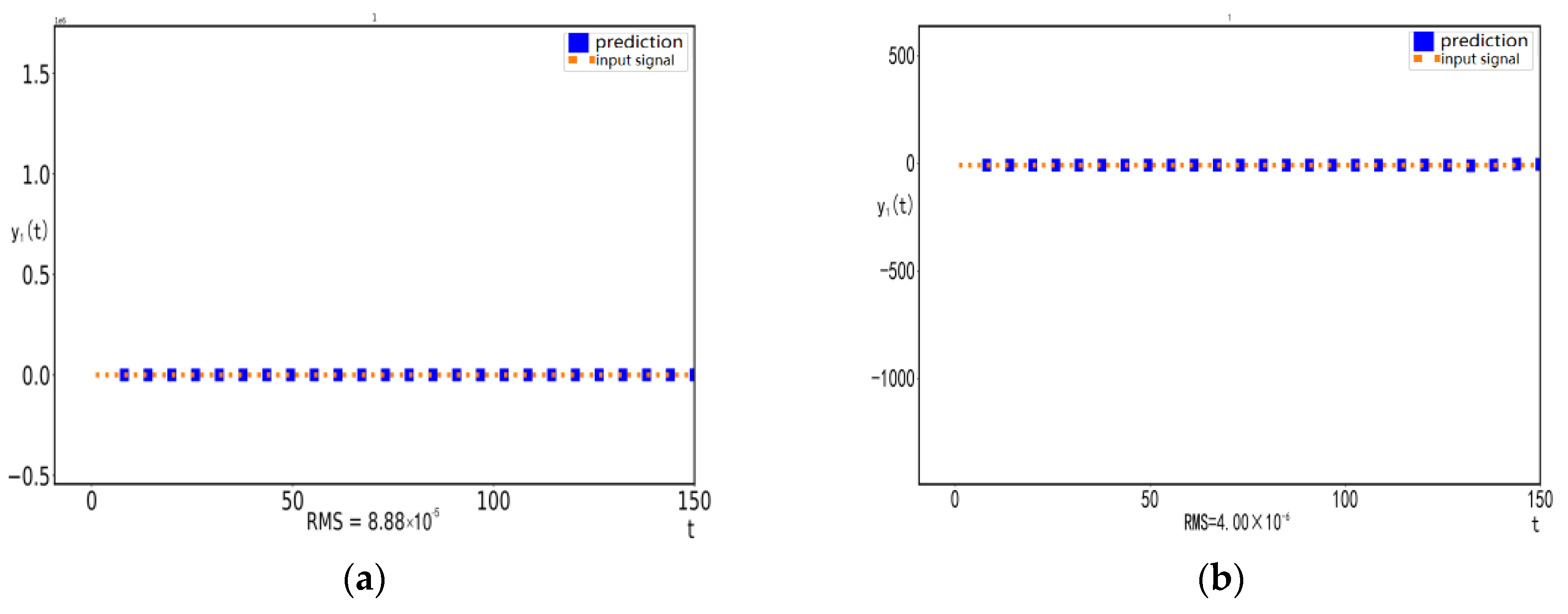
We first show the capability of the trained RC in predicting and replicating the dynamics of the ring-coupled Lorenz oscillators system. Setting $R=30$, the Lorenz oscillator system presents the fixed point motion. Following the same procedure as CRW, the reservoir is evolving in a closed-loop mode according to Equations (5) and (6) by replacing $u(t)$ with $v(t)$. Choosing the predicted value $y_1$ generated by TSI and OSI with a length of 200 to observe the reconstruction effect between the original system and the reconstructed system. To prove that the reservoir computer is well-trained, we choose to input the predicted value $y_1$ generated by TSI and OSI when $t=6$ as shown in Figure 2a,b. We find that the predicted trajectory is consistent with the original system after $t=6$. The RMS results show that the reconstruction effects of the two response systems are very good, and corresponding the RMS are $8.88\times {10}^{-5}$ and $4.00\times {10}^{-6}$ respectively, and the reconstruction effect of OSI is better than TSI. Similarly, when $R$ is greater than 29 and less than 30.48, the motion state of the fixed point can be maintained well in the reservoir computer. Moreover, the dynamic behavior of the TSI and OSI near the bifurcation point can also be well preserved in the reconstruction process. It shows that the reconstructed system has the same bifurcation point $R=29.00$ as the original system.

4.2. Synchronous Chaos

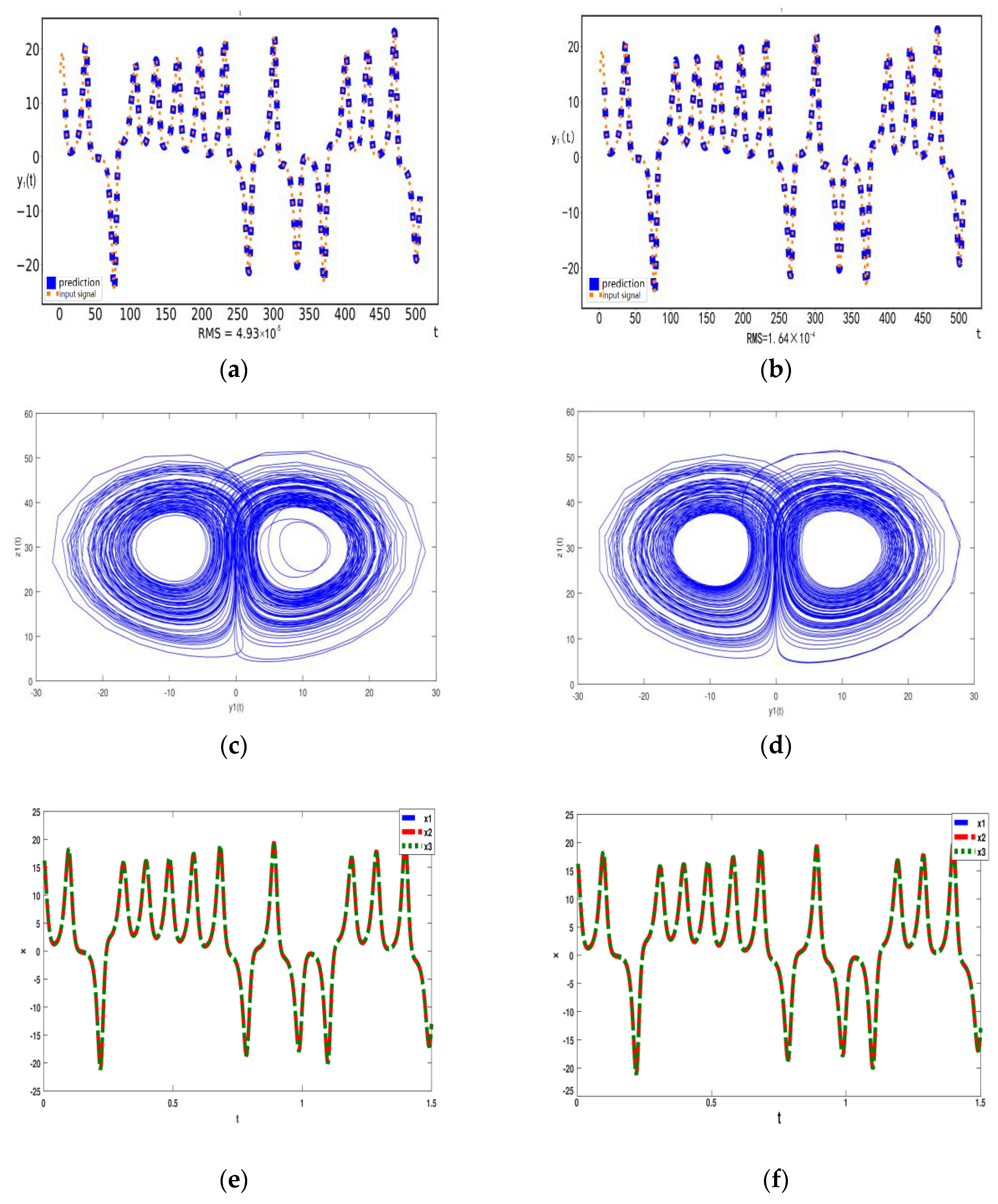
With the increase in $R$, the ring coupled Lorenz oscillator system will transition to chaotic synchronization motion at 30.49. Setting $R=31.0$, following the same procedure as CRW, in Figure 3a,b, we first choose the predicted value $y_1$ generated by TSI and OSI with a length of 500 to observe the reconstruction effect between the original system and the reconstructed system. We find that the predicted trajectory obtained from TSI and OSI is consistent with the trajectory of the original system after $t=6$, and corresponding the RMS are $4.93\times {10}^{-5}$ and $1.64\times {10}^{-4}$, respectively. The results of RMS clearly show that the reconstruction effect of OSI is better than TSI.

We next demonstrate the replication of the system climate in the ring-coupled Lorenz oscillators system, as depicted in Figure 3c,d. We chose the predicted variables $y_1$ and $z_1$ generated by TSI and OSI with a length of 5000 to show the chaos. To confirm further the replication of the system climate, we calculate the largest Lyapunov exponent (LE) of the original system and TSI and OSI, respectively, by the numerical method proposed in [34]. The LE for system (1) is 1.77, and the LE for TSI and OSI is 1.87 and 1.62, respectively. This shows that the trained RC not only accurately predicts the short-term evolution of the system (1) but also properly replicates the coupled Lorenz system climate.

Here, we want to demonstrate that the spatio-temporal structure can also maintain in the reconstruction process. We choose the predicted variables $x_i(i=1,2,3)$ generated by TSI and OSI with a length of 500 to show the motion state between oscillators, as shown in Figure 3e,f. We find that there is no phase difference between the motion trajectories represented by variable $x_i(i=1,2,3)$ of the two reconstructed systems, which shows that the spatio-temporal structure is still maintained in the reconstruction process. Similarly, when $R$ is greater than 30.48 and less than 32.99, the motion state of the synchronous chaos can be maintained well in the reservoir computer. Moreover, the dynamic behavior of the TSI and OSI near the bifurcation point can also be well preserved in the reconstruction process. It shows that the reconstructed system has the same bifurcation point $R=30.49$ as the original system.

4.3. Chaotic Rotating Wave

The chaotic rotating wave motion occurs at 32.99. It means that chaotic motion exists at the same time as an oscillation with a phase difference of $\frac{2\pi }{\mathrm{n}}$ between adjacent units. This corresponds to $Q_1-Q_2$ satisfying the rotating periodic condition.

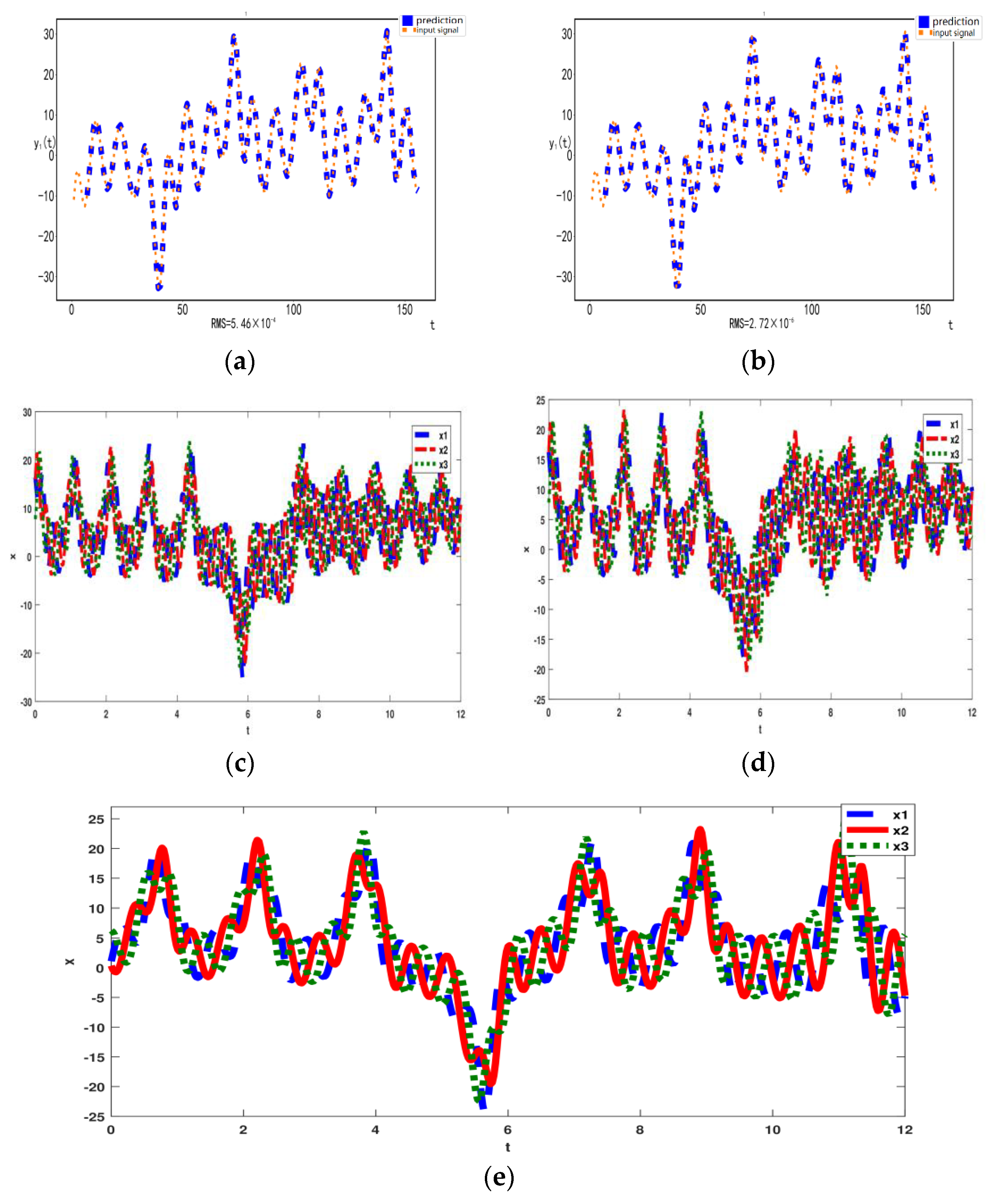
The trained reservoir system can infer the trajectory of the ring-coupled Lorenz oscillators system accurately. For the TSI, where we show the $y_1$ variable with a length of 100 as an example, see Figure 4a. Then we use the $x_1$, $x_2$ and $x_3$ component of the ring coupled Lorenz oscillators system as the driving signal for which the input vector fed into the training reservoir computer becomes $u(t)={(x_1,y_1^{\prime },z_1^{\prime },x_2,y_2^{\prime },z_2^{\prime },x_3,y_3^{\prime },z_3^{\prime })}^T$, where the initial values of $y_1^{\prime }(0),z_1^{\prime }(0),y_2^{\prime }(0),$$z_2^{\prime }(0),y_3^{\prime }(0),z_3^{\prime }(0)$ are chosen randomly. Based on Equations (5) and (6), we can generate the subsequent values $x_1,y_1^{\prime },z_1^{\prime },x_2,y_2^{\prime },z_2^{\prime },$ $x_3,y_3^{\prime },z_3^{\prime }$ autonomously for which the output vector $v(t)=(x_1^{\prime }(t),y_1^{\prime }(t),z_1^{\prime }(t),x_2^{\prime }(t),$ $y_2^{\prime }(t),z_2^{\prime }(t),x_3^{\prime }(t),y_3^{\prime }(t),z_3^{\prime }(t){)}^T$ of the reservoir computer is used as the next input vector $u(t+1)={(x_1(t),y_1^{\prime }(t),z_1^{\prime }(t),x_2(t),y_2^{\prime }(t),z_2^{\prime }(t),x_3(t),y_3^{\prime }(t),z_3^{\prime }(t))}^T$ with the $x_1^{\prime }(t)$, $x_2^{\prime }(t)$ and $x_3^{\prime }(t)$ replaced by the driving signals $x_1(t)$, $x_2(t)$ $x_3(t)$. For the OSI, where we show the $y_1$ variable with a length of 100 as an example, see Figure 4b. Then we use the $x_1$ component of the ring-coupled Lorenz oscillators system as the driving signal for which the input vector fed into the training reservoir computer becomes $u(t)={(x_1,y_1^{\prime },z_1^{\prime },x_2^{\prime },y_2^{\prime },z_2^{\prime },x_3^{\prime },y_3^{\prime },z_3^{\prime })}^T$, where the initial values of $y_1^{\prime }(0),z_1^{\prime }(0),x_2^{\prime }(0),y_2^{\prime }(0),z_2^{\prime }(0),x_3^{\prime }(0),y_3^{\prime }(0),z_3^{\prime }(0)$ are chosen randomly. Based on Equations (5) and (6), we can generate the subsequent values $x_1,y_1^{\prime },z_1^{\prime },x_2^{\prime },$ $y_2^{\prime },z_2^{\prime },x_3^{\prime },y_3^{\prime },z_3^{\prime }$ autonomously for which the output vector $v(t)=(x_1^{\prime }(t),y_1^{\prime }(t),z_1^{\prime }(t),x_2^{\prime }(t),y_2^{\prime }(t),z_2^{\prime }(t),$$x_3^{\prime }(t),y_3^{\prime }(t),z_3^{\prime }(t){)}^T$ of the reservoir computer is used as the next input vector $u(t+1)={(x_1(t),y_1^{\prime }(t),z_1^{\prime }(t),x_2^{\prime }(t),y_2^{\prime }(t),z_2^{\prime }(t),x_3^{\prime }(t),y_3^{\prime }(t),z_3^{\prime }(t))}^T$ with $x_1^{\prime }(t)$ replaced by the driving signal $x_1(t)$. Interestingly, we find the predicted trajectory obtained from TSI and OSI is consistent with the trajectory of the original system after $t=6$. It shows that the TSI and OSI provided by the trained reservoir system will synchronize with a driving system provided by the coupled Lorenz system and correspond to the RMS are $5.46\times {10}^{-4}$ and $2.72\times {10}^{-6}$ respectively. The results of RMS clearly show that the reconstruction effect of OSI is better than TSI. The same procedure is followed in other experiments.

Meanwhile, we want to demonstrate that the rotational symmetric structure of CRW can also maintain in the reconstruction process. We choose the predicted variables $x_i(i=1,2,3)$ generated by TSI and OSI with a length of 500 to show the motion state between oscillators, as depicted in Figure 4c,d. We can see when $t\le 8$, the trajectories of the original system and reconstructed systems’ trajectories are the same. When $t\succ 8$, the trajectories of the original system and the reconstructed system begin to be inconsistent. Although the reconstructed system is inconsistent with the original system, we find that the phase difference between the oscillators in the reconstructed system remains the same, which indicates that the spatio-temporal structure of TSI and OSI can be consistent with the original system. To confirm further the replication of the system climate, we calculate the LE of TSI and OSI that correspond to 1.51 and 1.60, respectively. The LE for the system (1) is 1.82. This shows that even though the reservoir computer is well-trained, it cannot make long-term predictions. However, it can replicate the couple Lorenz system climate. Similarly, when $R$ is greater than 32.99 and less than 35.08, the motion state and spatio-temporal structure of chaotic rotating waves are well maintained in the reconstruction process. Moreover, the dynamic behavior of the TSI and OSI near the bifurcation point can also be well preserved in the reconstruction process. It shows that the reconstructed system has the same bifurcation point $R=32.99$ as the original system.

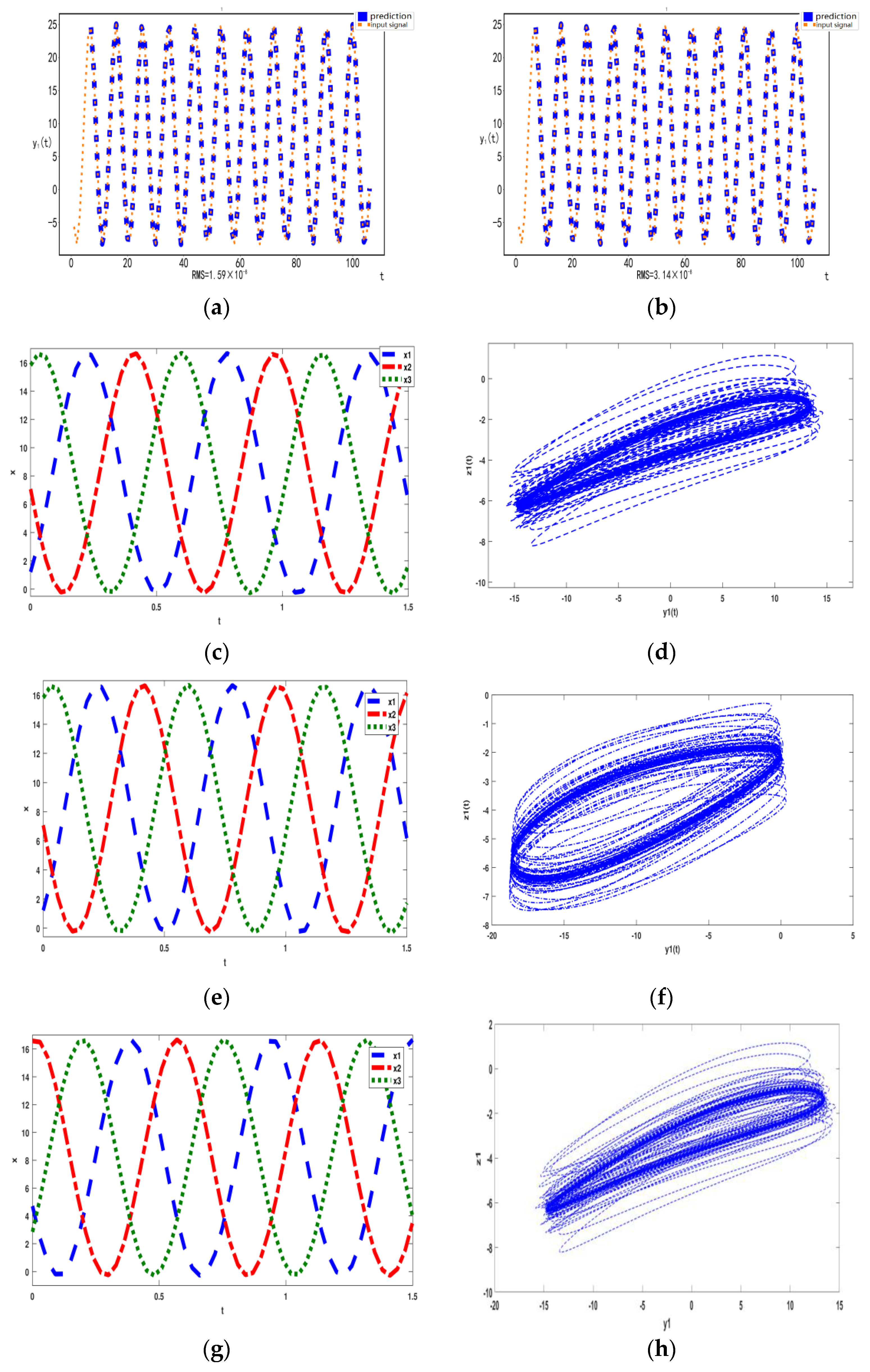
4.4. Periodic Rotating Wave

The periodic rotating wave motion occurs at 35.09. This state is characterized by a fast periodic motion of the oscillators of the array and phase differences of $\frac{2\pi }{3}$ between adjacent oscillators. In Figure 5a,b, we show the variable $y_1$ with the length of 100 of the reconstructed and original systems to observe the reconstruction effect. Interestingly, if we set the system to evolve in a closed loop after $t=6$, we find that the predicted trajectory obtained from TSI and OSI is consistent with the trajectory of the original system immediately. This shows that reconstruction of TSI and OSI and the ring-coupled Lorenz system can be achieved. Meanwhile, corresponding to the root mean square is $1.59\times {10}^{-8}$ and $3.14\times {10}^{-8}$, respectively. The results of RMS more clearly show that the reconstruction effect of OSI is better than TSI.

In Figure 5c,e, we choose the predicted variables $x_i(i=1,2,3)$ generated by TSI and OSI with a length of 100 to show the motion state between oscillators. Compared with Figure 5g, we find that the phase difference between the Lorenz oscillators in TSI and OSI is $\frac{2\pi }{3}$ which is consistent with the original system. This shows that the spatio-temporal structure of the TSI and OSI can be maintained in the reconstruction process. Then we chose the predicted variables $y_1$ and $z_1$ generated by TSI and OSI with a length of $1\times {10}^4$ to reconstruct the phase diagram of the original system, as depicted in Figure 5d,f. Compared with the phase diagram of the original system, we find that it can maintain the periodic behavior of the system (1). Similarly, when $R$ is greater than 35.09 and less than 38.00, the motion state of the periodic rotating wave can be maintained well in the reconstruction process. Moreover, the motion state and spatio-temporal structure of PRW of the TSI and OSI near the bifurcation point can also be well preserved in the reconstruction process. It shows that the reconstructed system has the same bifurcation point $R=35.09$ as the original system.

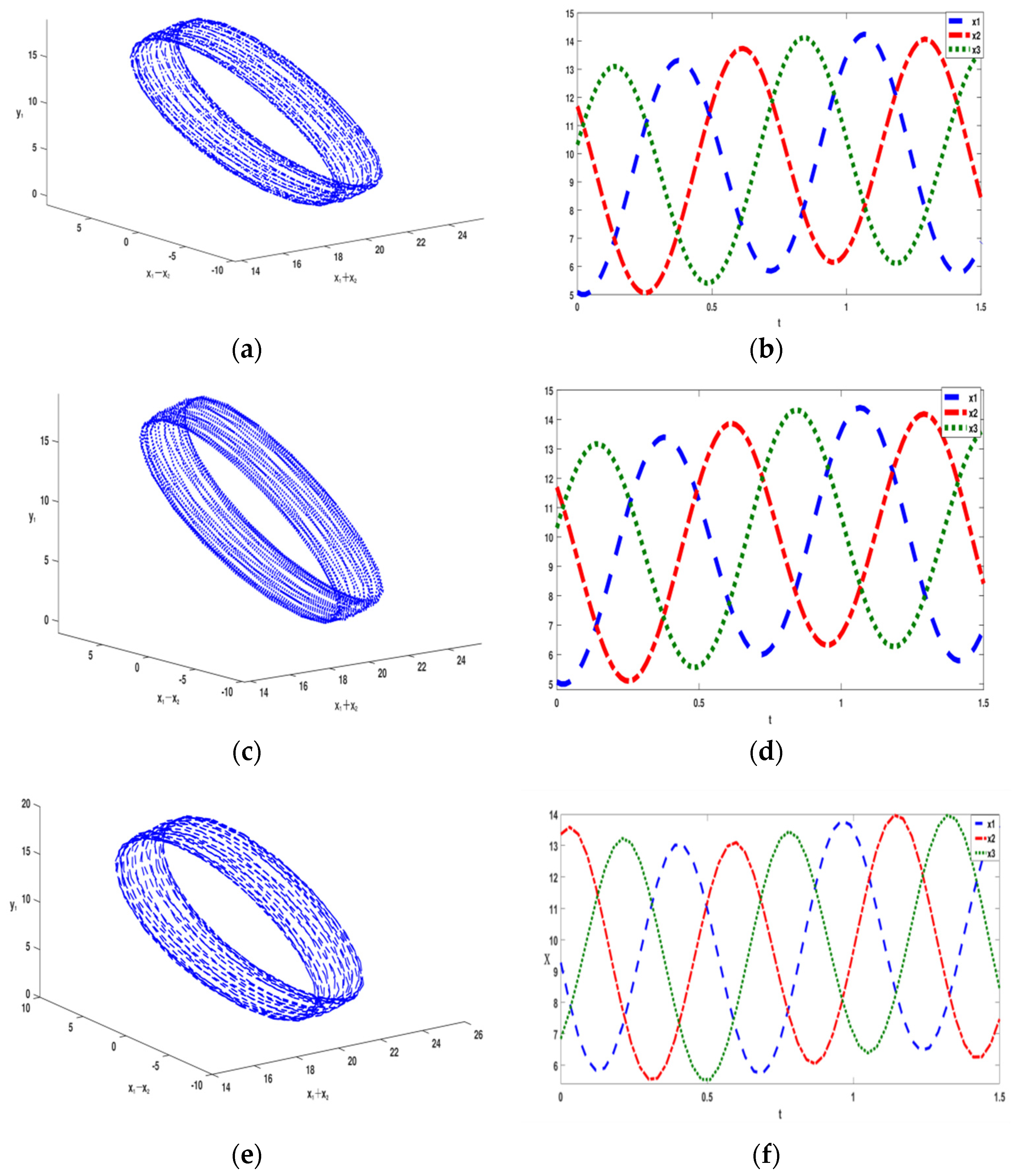
4.5. Quasi-Periodicity

The two Hopf bifurcation points are so close that the second Hopf bifurcation leads to quasi-periodicity. The invariant torus is shown in Figure 6 when $R=35.26$.

In Figure 6b,d, we choose the predicted variables $x_i(i=1,2,3)$ generated by TSI and OSI with a length of 100 to show the motion state between oscillators. Compared with Figure 6f, we find that the phase difference between TSI and OSI is consistent with the original system. In Figure 6a,c, we used the predicted values $x_1$, $x_2$, and $y_1$ with a length of $1\times {10}^4$ obtained from TSI and OSI to show the spatio-temporal structure. This shows that the spatio-temporal structure of the TSI and OSI can be maintained in the reconstruction process. Similarly, when $R$ is greater than 35.09 and less than 35.29, the motion state of the quasi-periodicity wave can be maintained well in the reconstruction process. Moreover, the motion state and spatio-temporal structure of quasi-periodicity of the TSI and OSI near the bifurcation point can also be well preserved in the reconstruction process. It shows that the reconstructed system has the same bifurcation point of 38.00 as the original system.

5. Discussion

In this paper, we focus on the principle of synchronization between systems and the idea of reservoir computing to study reconstruction problems on various dynamical behaviors in unidirectional coupled Lorenz systems, including a stable point, periodic rotating wave, synchronous chaos, chaos rotating wave, and invariant torus. In the numerical experiment, we take the three oscillator systems as an example to prove that the symmetrical double-layer coupling network can well learn the above dynamic behaviors by sharing only the information of one Lorenz oscillator of the original system, and the results of RMS clearly show that the reconstruction effect of OSI is better than that of TSI for all the above attractors. Similarly, the original system can be reconstructed well by sharing a small amount of information in complex networks connected by multiple oscillators. We also show that the well-trained reservoir computer cannot make long-term predictions in the process of coupled oscillator system reconstruction, but it can replicate the ergodicity of the system in the process of reconstruction. Meanwhile, the motion near the bifurcation point of the transition between attractors can also be well preserved. Most importantly, we also confirmed that the spatio-temporal structure of the above attractors could be well maintained in the reconstruction process, especially the rotational symmetry of CRW, quasi-periodic torus, and PRW.

These findings reveal that although the prediction data in the long-term will deviate from the original system, the underlying spatio-temporal structure is preserved in the trained reservoir computer. The original reservoir computing cannot deal with the change of parameter value. Therefore, the reconstruction of different attractors of the same system needs to be studied and predicted many times. This also lays a foundation for selecting an appropriate reservoir computer to reconstruct the above dynamics in the future. For example, we can reconstruct the above dynamic behavior by constructing a parameter-aware RC with high precision by tuning a control parameter externally.

References

- Pecora, L.M.; Carroll, T.L. Synchronization in Chaotic Systems. Phys. Rev. Lett. 1990, 64, 821–824. [Google Scholar] [CrossRef] [PubMed]
- Rosenblum, M.G.; Pikovsky, A.S.; Kurths, J. Phase Synchronization of Chaotic Oscillators. Phys. Rev. Lett. 1996, 76, 1804–1807. [Google Scholar] [CrossRef] [PubMed]
- Lai, Y.C.; Grebogi, C. Synchronization of chaotic trajectories using control. Phys. Rev. E 1993, 47, 2357–2360. [Google Scholar] [CrossRef] [PubMed]
- Boccaletti, S.; Kurths, J.; Osipov, G.; Valladares, D.L.; Zhou, C.S. The synchronization of chaotic systems. Phys. Rep. 2002, 366, 1–101. [Google Scholar] [CrossRef]
- Fujisaka, H.; Yamada, T. Stability theory of synchronized motion in coupled-oscillator systems. Prog. Theor. Phys. 1983, 69, 32–47. [Google Scholar] [CrossRef]
- Fujisaka, H.; Yamada, T. Stability theory of synchronized motion in coupled-oscillator systems. IV. Prog. Theor. Phys. 1985, 74, 918–921. [Google Scholar] [CrossRef] [Green Version]
- Fujisaka, H.; Yamada, T. Stability theory of synchronized motion in coupled-oscillator systems. II. Prog. Theor. Phys. 1983, 70, 1240–1248. [Google Scholar]
- Fujisaka, H.; Yamada, T. Stability theory of synchronized motion in coupled-oscillator systems. III. Prog. Theor. Phys. 1984, 72, 885–894. [Google Scholar]
- Boccaletti, S.; Valladares, D.L.; Pecora, L.M.; Geffert, H.; Carroll, T.L. Reconstructing embedding spaces of coupled dynamical systems from multivariate data. Phys. Rev. E 2002, 65, 035204. [Google Scholar] [CrossRef] [Green Version]
- Jaeger, H.; Haas, H. Harnessing Nonlinearity: Predicting Chaotic Systems and Saving Energy in Wireless Communication. Science 2004, 304, 78–80. [Google Scholar] [CrossRef] [Green Version]
- Pathak, J.; Lu, Z.X.; Hunt, B.; Girvan, M.; Ott, E. Using machine learning to replicate chaotic attractors and calculate Lyapunov exponents from data. Chaos 2017, 12, 121102. [Google Scholar] [CrossRef] [PubMed]
- Pathak, J.; Hunt, B.; Girvan, M.; Lu, Z.X.; Ott, E. Model-Free Prediction of Large Spatiotemporally Chaotic Systems from Data: A Reservoir Computing Approach. Phys. Rev. Lett. 2018, 120, 024102. [Google Scholar] [CrossRef] [PubMed] [Green Version]
- Chen, X.L.; Weng, T.F.; Yang, H.J.; Gu, C.G.; Zhang, J.; Small, M. Mapping topological characteristics of dynamical systems into neural networks: A reservoir computing approach. Phys. Rev. E 2020, 102, 033314. [Google Scholar] [CrossRef] [PubMed]
- Griffith, A.; Pomerance, A.; Gauthier, D.J. Forecasting chaotic systems with very low connectivity reservoir computers. Chaos 2019, 29, 123108. [Google Scholar] [CrossRef] [PubMed] [Green Version]
- Zimmermann, R.S.; Parlitz, U. Observing spatio-temporal dynamics of excitable media using reservoir computing. Chaos 2018, 28, 043118. [Google Scholar] [CrossRef] [Green Version]
- Carroll, T.L. Using reservoir computers to distinguish chaotic signals. Phys. Rev. E 2018, 98, 052209. [Google Scholar] [CrossRef] [Green Version]
- Jiang, J.J.; Lai, Y.C. Model-free prediction of spatiotemporal dynamical systems with recurrent neural networks: Role of network spectral radius. Phys. Rev. Res. 2019, 1, 033056. [Google Scholar] [CrossRef] [Green Version]
- Follmann, R.; Rosa, E. Predicting slow and fast neuronal dynamics with machine learning. Chaos 2019, 29, 113119. [Google Scholar] [CrossRef]
- Jaeger, H.; Lukoševičius, M. Reservoir computing approaches to recurrent neural network training. Comput. Sci. Rev. 2009, 3, 127–149. [Google Scholar]
- Lu, Z.X.; Hunt, B.; Ott, E. Attractor reconstruction by machine learning. Chaos 2018, 28, 061104. [Google Scholar] [CrossRef] [Green Version]
- Zhang, H.; Fan, H.W.; Wang, L.; Wang, X.G. Learning Hamiltonian dynamics with reservoir computing. Phys. Rev. E 2021, 104, 024205. [Google Scholar] [CrossRef] [PubMed]
- Sánchez, E.; Pazó, D.; Matías, M.A. Experimental study of the transitions between synchronous chaos and a periodic rotating wave. Chaos 2006, 16, 033122. [Google Scholar] [CrossRef] [Green Version]
- Sánchez, E.; Matías, M.A. Transition to rotating chaotic waves in arrays of coupled Lorenz oscillators. Int. J. Bifurc. Chaos 1998, 9, 2335–2343. [Google Scholar] [CrossRef] [Green Version]
- Wang, S.; Yang, X.; Li, Y. The mechanism of rotating waves in a ring of unidirectionally coupled Lorenz systems. Commun. Nonlinear Sci. 2020, 90, 105370. [Google Scholar] [CrossRef]
- Wang, S.; Yang, X.; Li, Y. Synchronization or cluster synchronization in coupled Van der Pol oscillators networks with different topological types. Phys.Scr. 2022, 97, 035205. [Google Scholar]
- Wang, S.; Li, Y.; Yang, X. Synchronization, symmetry and rotating periodic solutions in oscillators with Huygens’ coupling. Physica D 2022, 434, 133208. [Google Scholar]
- Horikawa, Y. Metastable and chaotic transient rotating waves in a ring of unidirectionally coupled bistable Lorenz systems. Physica D 2013, 261, 8–18. [Google Scholar] [CrossRef]
- Liu, G.G.; Li, Y.; Yang, X. Rotating periodic solutions for asymptotically linear second-order Hamiltonian systems with resonance at infinity. Math. Methods Appl. Sci. 2017, 40, 7139–7150. [Google Scholar] [CrossRef]
- Liu, G.G.; Li, Y.; Yang, X. Existence and multiplicity of rotating periodic solutions for resonant Hamiltonian systems. J. Differ. Equ. 2018, 265, 1324–1352. [Google Scholar] [CrossRef]
- Yang, X.; Zhang, Y.; Li, Y. Existence of rotating-periodic solutions for nonlinear systems via upper and lower solutions. Rocky Mt. J. Math. 2017, 47, 2437–2452. [Google Scholar] [CrossRef]
- Pecora, L.M.; Carroll, T.L. Synchronization in Chaotic Systems. Chaos 2015, 25, 097611. [Google Scholar] [CrossRef] [PubMed]
- Roman, R.C.; Precup, R.E.; Petriu, E.M. Hybrid data-driven fuzzy active disturbance rejection control for tower crane systems. Eur. J. Control. 2020, 08, 001. [Google Scholar] [CrossRef]
- Chi, R.H.; Li, H.Y.; Shen, D.; Hou, Z.S.; Huang, B. Enhanced P-type Control: Indirect Adaptive Learning from Set-point Updates. IEEE Trans. Autom. Control 2022. [Google Scholar] [CrossRef]
- Sano, M.; Sawada, Y. Measurement of the Lyapunov spectrum from a chaotic time series. Phys. Rev. Lett. 1985, 55, 1082–1085. [Google Scholar] [CrossRef]
Figure 1.
(a,b) show the two types of drive-response systems. The circles and their labels represent the dynamic variables of the systems and the connections represent couplings. represent the Lorenz oscillators and represent the driven signals. The double-layer coupled networks are shown: (a) is the drive-response system of three signals input , (b) the drive-response system of one signal input .
Figure 2.
(a) The time evolution of TSI and the original system. (b) The time evolution of OSI and the original system. Prediction starts at . The following settings are the same. Results obtained by the original system are colored in red and predicted by RC are colored in blue.
Figure 3.
(a) The time evolution of TSI and the original system. (b) The time evolution of OSI and the original system. (c) The phase diagram of TSI. (d) The phase diagram of OSI. (e) The Phase difference diagram of variables from TSI. (f) The Phase difference diagram of variables from OSI. Results obtained by the original system are colored in red and predicted by RC are colored in blue.
Figure 4.
(a) The time evolution of TSI and the original system. (b) The time evolution of OSI and the original system. (c) The Phase difference diagram of variables from TSI. (d) The Phase difference diagram of variables from OSI. (e) The phase difference diagram of the original system. Results obtained by the original system are colored in red and predicted by RC are colored in blue.
Figure 5.
(a) The time evolution of the TSI and the original system. (b) The time evolution of the OSI and the original system. (c) The Phase difference diagram of variables from TSI. (d) The Phase diagram of TSI single oscillator structure. (e) The Phase difference diagram of variables from OSI. (f) The Phase diagram of OSI single oscillator structure. (g) The Phase difference diagram of variables from the original system. (h) The Phase diagram of the original system single oscillator structure. Results obtained by the original system are colored in red and predicted by RC are colored in blue.
Figure 6.
(a) The quasi-periodic invariant torus of TSI. (b) The Phase difference diagram of variables from TSI. (c) The quasi-periodic invariant torus of OSI. (d) The Phase difference diagram of variables from OSI. (e) The quasi-periodic invariant torus of the original system. (f) The Phase difference diagram of variables from the original system.