Analytical Formulas for Conditional Mixed Moments of Generalized Stochastic Correlation Process

Abstract

This paper proposes a simple and novel approach based on solving a partial differential equation (PDE) to establish the concise analytical formulas for a conditional moment and mixed moment of the Jacobi process with constant parameters, accomplished by including random fluctuations with an asymmetric Wiener process and without any knowledge of the transition probability density function. Our idea involves a system with a recurrence differential equation which leads to the PDE by involving an asymmetric matrix. Then, by using Itô’s lemma, all formulas for the Jacobi process with constant parameters as well as time-dependent parameters are extended to the generalized stochastic correlation processes. In addition, their statistical properties are provided in closed forms. Finally, to illustrate applications of the proposed formulas in practice, estimations of parametric methods based on the moments are mentioned, particularly in the method of moments estimators.

1. Introduction

The diffusion process has been studied thoroughly in seeking a solution for a stochastic differential equation (SDE) as well as for its properties, such as the conditional moments and mixed moments, which play significant roles in various applications and are especially beneficial for the estimation of rate parameters. Usually, these moments can be directly evaluated by utilizing the transition probability density function (PDF), which is sometimes unknown, complicated, or unavailable in closed form. Hence, the analytical formula for the moments of the SDE may be unavailable. The important application of these moments is parameter estimation. There are many tools to estimate parameters, such as the maximum likelihood estimator (MLE), which is one of the most efficient tools. Sometimes, however, it cannot be performed directly for the data of processes for which the transition PDFs are unknown or complicated. Thus, the moments are required for estimating parameters; this can be performed via several methods, e.g., martingale estimating functions, quasi-likelihood methods, nonlinear weighted least squares estimation, and method of moments (MM).

The aim of this paper is mainly to propose a simple analytical formula for conditional mixed moments of a generalized stochastic correlation process without requiring the transition PDF. As for more specific details, we let $\left(\Omega ,{\mathcal{F}}_s,{\left\{{\mathcal{F}}_s\right\}}_{0\le s\le T_1\le T_2},P\right)$ be a filtered probability space generated by an adapted stochastic process ${\left\{{\rho }_t\right\}}_{s\le t\le T_2}$. This paper focuses on the conditional expectation of a product of polynomial functions ${\rho }_{T_1}^{n_1}$ and ${\rho }_{T_2}^{n_2}$ of the form

$$\mathbb{E}\left[{\rho }_{T_1}^{n_1}{\rho }_{T_2}^{n_2}\mid {\mathcal{F}}_s\right]=\mathbb{E}\left[{\rho }_{T_1}^{n_1}{\rho }_{T_2}^{n_2}\mid {\rho }_s=\rho \right],$$

(1)

called a conditional mixed moment up to order $n_1+n_2$ for $n_1,n_2\in {\mathbb{Z}}_0^{+}$, the analytical formula of which has not been provided, where $\rho \in [{\rho }_{\min },{\rho }_{\max }]\subseteq \mathbb{R}$ and ${\rho }_t$ evolve according to a generalized stochastic correlation process (time-dependent parameters) governed by the following SDE:

$$d{\rho }_t={\theta }^{*}\left(t\right)\left({\mu }^{*}\left(t\right)-{\rho }_t\right)dt+{\sigma }^{*}\left(t\right)\sqrt{\left({\rho }_{\max }-{\rho }_t\right)\left({\rho }_t-{\rho }_{\min }\right)}d{W}_t,$$

(2)

where $W_t$ is an asymmetric Wiener process, ${\theta }^{*}\left(t\right)>0$, ${\sigma }^{*}\left(t\right)>0$, and ${\rho }_{\min }<{\mu }^{*}\left(t\right)<{\rho }_{\max }$ for all $t\in [s,T_2]$. The parameter ${\theta }^{*}\left(t\right)$ corresponds to the mean-reverting parameter, ${\mu }^{*}\left(t\right)$ represents the mean of the process, and ${\sigma }^{*}\left(t\right)$ is the volatility coefficient which determines the state space of the diffusion. Emmerich [1] showed that the stochastic correlation process, which is (2) when the parameters ${\theta }^{*}\left(t\right)$, ${\mu }^{*}\left(t\right)$, and ${\sigma }^{*}\left(t\right)$ are constant, ${\rho }_{\min }=-1$, and ${\rho }_{\max }=1$, fulfills the natural features which correlation is expected to possess. In fact, this process is a transformed version of the Jacobi process [2]. In other words, the Jacobi process is the generalized stochastic correlation process (2) when the parameters ${\theta }^{*}\left(t\right)$, ${\mu }^{*}\left(t\right)$, and ${\sigma }^{*}\left(t\right)$ are constant, ${\rho }_{\min }=0$, and ${\rho }_{\max }=1$. Moreover, the Jacobi process is commonly used to describe the dynamic of discretely sampled data with range $[0,1]$, such as the regime probability or default probability, discount coefficient, and arbitrage free pure discount bond price; see e.g., [2,3].

The conditional mixed moment (1) becomes the well-known conditional moment when ${\gamma }_1=0$. It is worth noting that the conditional moment, which is usually used in many branches of mathematical science (especially in describing the dynamics of observed data), has been studied extensively from a probabilistic viewpoint. 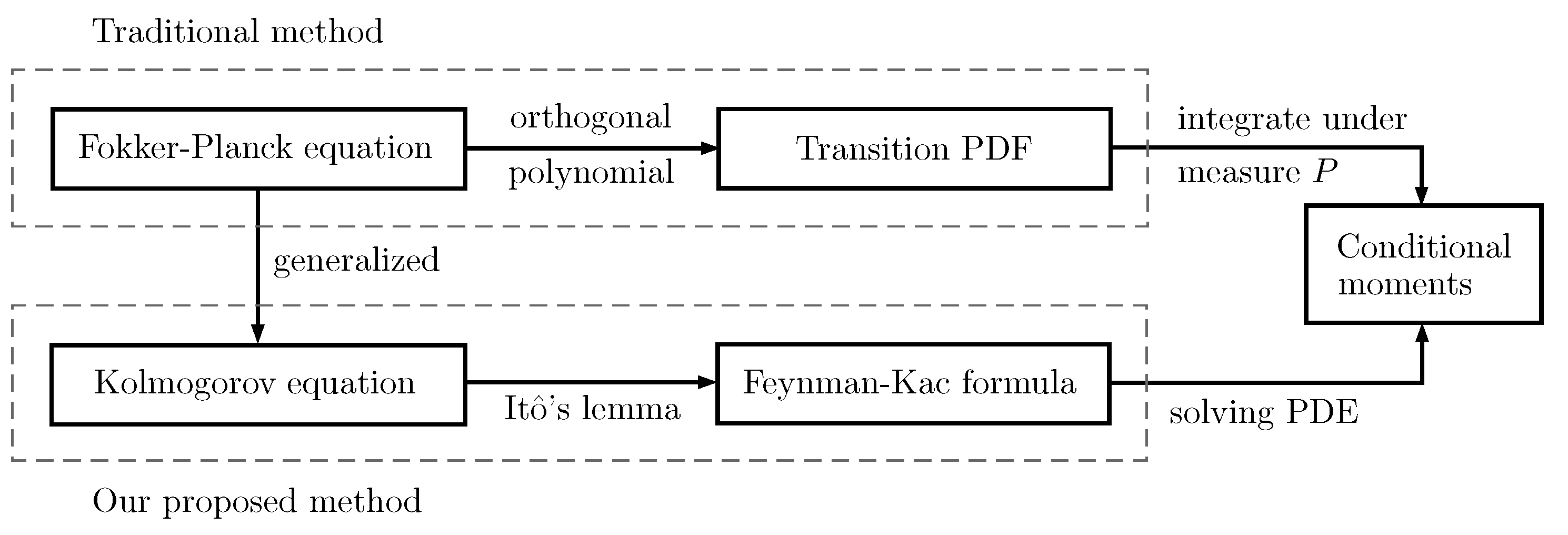In 2002, to study the moment evaluation of interest rates, Delbaen and Shirakawa [2] provided an analytical formula for the transition PDF of the Jacobi process through solving it using the orthogonal polynomials with the Fokker–Planck equation, called Jacobi polynomials. In addition, an analytical formula for the conditional moments of the Jacobi process was algebraically solved by applying the transition PDF; see Figure 1. The transition PDF of Jacobi process is very complicated and involves the Jacobi polynomials; their formula is difficult to work with, especially, when extending it to a formula for conditional mixed moments (1). The authors showed that the Jacobi process, which is bounded on $[0,1]$, becomes a more general bounded process on $[{\rho }_{\min },{\rho }_{\max }]$ by using Itô’s lemma; see more details in [2]. In this case, an analytical formula for conditional moments of the new bounded process is provided in [2] as well. In 2004, Gouriéroux and Valéry [3] proposed a method to find the conditional mixed moments in order to calibrate the values of parameters on well conditional moments. Their idea used the conditional power moments, sometimes called the tower property, on the conditional moments. However, their formula for the conditional moments is based on solving the system of conditional moments recursively.

In this work, by utilizing the Feynman–Kac formula, which is transformed from the Kolmogorov equation by using Itô’s lemma, we provide a simple analytical formula for conditional moments of the Jacobi process. The key interesting element of our work is that we successfully solve the partial differential equation (PDE) given in the Feynman–Kac formula, as shown in Figure 1. The obtained formula does not require solving any recursive system, as is the case in the literature to date. In addition, by applying the obtained formula with the binomial theorem, we immediately obtain a simple analytical formula for conditional moments of the generalized stochastic correlation process (2). Moreover, we extend the obtained formulas to the conditional mixed moments (1) using the tower property. We propose an analytical formula for several mathematical properties, such as the conditional variance, covariance, central moment and correlation, as consequences of our results.

The overall idea of our results relies on a PDE solution provided by the Feynman–Kac formula, which corresponds to the solution of (1). Roughly speaking, by assuming the solution of the PDE as a polynomial expression, we can solve the coefficients to receive a closed-form formula directly. The key motivation for the form of conditional moments, that is, a solution to PDE, is based on [4,5,6,7]. Because the SDE in the Jacobi process has linear drift coefficient and polynomial squared diffusion coefficient, the closed-form solutions of the conditional moments can be assumed by the polynomial expansion; see more details in [4,8,9,10,11].

The rest of this paper is organized as follows. Section 2 provides a brief overview of the extended Jacobi process and the generalized stochastic correlation process. The key methodology and main theorems are proposed in Section 3. Experimental validations of proposed formulas are shown in Section 4 via Monte Carlo (MC) simulations. To illustrate applications in practice, parameter estimation methods based on conditional moments are mentioned in Section 5.

2. Jacobi and Generalized Stochastic Correlation Processes

The Jacobi process is a class of solvable diffusion processes the solution of which satisfies the Pearson equation [12]. It involves a wide variety of issues in many branches, such as chemistry, physics and engineering; see more details in [13]. Over the past decade, the Jacobi process has been considered as one class of the Pearson diffusion process [4], sometimes called a generalized Jacobi process. The Pearson diffusion process is presented via an Itô process having linear drift coefficient and diffusion in quadratic square, which its dynamics follows:

$$d{X}_t=\theta \left(\mu -X_t\right)dt+\sqrt{2\theta \left(a{X}_t^2+b{X}_t+c\right)}d{W}_t,$$

(3)

where $W_t$ is an asymmetric Wiener process, $X_t$ is in state space, $\theta >0$, and a, b, and c are constants which ensure that the quadratic squared diffusion coefficient in (3) is well-defined for all t in time space. By considering the transition PDF of the Pearson diffusion process through the Fokker–Planck equation, Forman and Sørensen [4] classified it based on the stationary solution into six classes, including the Jacobi process.

Under the classification of Forman and Sørensen [4], the Pearson diffusion process becomes the Jacobi process under conditions $a<0$ and $b^2-4ac>0$. The simplest form of the Jacobi process follows the SDE (3) when $a=-b<0$ and $c=0$, and its dynamics follow

$$d{X}_t=\theta \left(\mu -X_t\right)dt+\sqrt{2a\theta X_t\left(X_t-1\right)}d{W}_t.$$

(4)

Unlike the Cox–Ingersoll–Ross process [14], which is only bounded below, all values produced from the Jacobi process (4) are bounded both below and above. To avoid inaccessible boundary points 0, 1, almost certain with respect to probability measure P, we need a sufficient condition that is $-a\le \mu \le 1+a$; see e.g., [2,15]. Under this condition, a generalized case of the Jacobi process (4) can be obtained by applying Itô’s lemma with ${\rho }_t={\rho }_{\min }+\left({\rho }_{\max }-{\rho }_{\min }\right)X_t$. In this work, we call this the generalized stochastic correlation process (constant parameters) governed by the SDE

$$d{\rho }_t=\theta \left(\left({\rho }_{\max }-{\rho }_{\min }\right)\mu +{\rho }_{\min }-{\rho }_t\right)dt+\sqrt{2a\theta \left({\rho }_t-{\rho }_{\max }\right)\left({\rho }_t-{\rho }_{\min }\right)}d{W}_t.$$

(5)

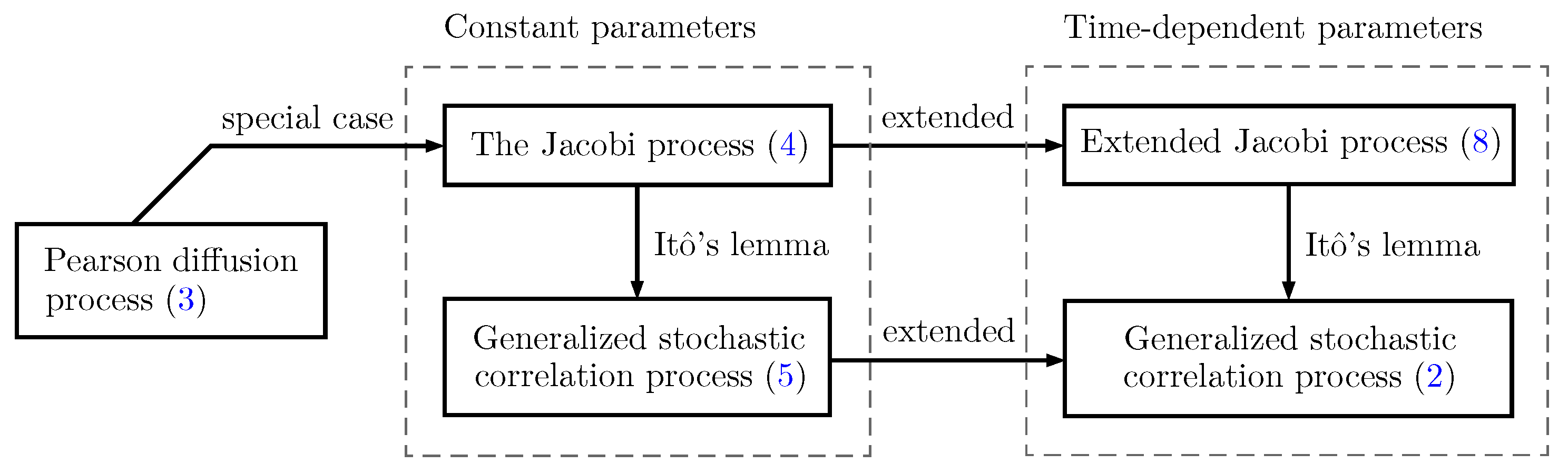
Comparing (2) with (5) yields ${\theta }^{*}\left(t\right)=\theta$, ${\mu }^{*}\left(t\right)=\left({\rho }_{\max }-{\rho }_{\min }\right)\mu +{\rho }_{\min }$ and ${\sigma }^{*}\left(t\right)=\sqrt{-2a\theta }$. Figure 2 summarizes the relation among processes (2)–(5) and (8). However, we return to the extended Jacobi process (8) again in Section 3.

In the context of conditional expectation, a rising question is whether the conditional expectation can be calculated directly by using the transition PDF. We begin with the transition PDF of the Jacobi process, which is associated with the Jacobi polynomials through the Jacobi generator’s eigenfunctions; see more details in [16,17]. In this case, we discuss only the simplest case provided in (4). We use the transition PDF following Leonenko’s version [17], which can be rewritten as

$$p(x,T\mid x_t,t)=beta\left(x\right)\sum _{j=0}^{\infty }\frac{e^{-{\lambda }_j(T-t)}}{{\omega }_j}{P}_j^{(\alpha ,\beta )}\left(2x_t-1\right)P_j^{(\alpha ,\beta )}\left(2x-1\right),$$

(6)

where $beta\left(x\right)=\frac{x^{\beta }{\left(1-x\right)}^{\alpha }}{\mathcal{B}\left(\alpha +1,\beta +1\right)}$ is the invariant distribution, $\mathcal{B}\left(\alpha ,\beta \right)=\frac{\mathrm{\Gamma }\left(\alpha \right)\mathrm{\Gamma }\left(\beta \right)}{\mathrm{\Gamma }\left(\alpha +\beta \right)}$ is the beta function, and $\mathrm{\Gamma }(·)$ is the gamma function

$$\left.\begin{array}{cc}\hfill & \alpha =-\frac{1}{a}+\frac{\mu }{a}-1,\beta =-\frac{\mu }{a}-1,{\lambda }_j=-ja\theta \left(j-1-\frac{1}{a}\right),{\omega }_0=1,\hfill \\ \hfill & {\omega }_j=\frac{\mathrm{\Gamma }\left(\alpha +2\right)\mathrm{\Gamma }\left(\beta +2\right)\mathrm{\Gamma }\left(\alpha +\beta +4-j\right)}{j!\mathrm{\Gamma }\left(\alpha +2-j\right)\mathrm{\Gamma }\left(\beta +2-j\right)\mathrm{\Gamma }\left(\alpha +\beta +3\right)\left(2j+\alpha +\beta +1\right)}\mathrm{and}\hfill \\ \hfill & P_j^{(\alpha ,\beta )}\left(z\right)=\frac{\mathrm{\Gamma }\left(\alpha +j+1\right)}{j!\mathrm{\Gamma }\left(\alpha +\beta +j+1\right)}\sum _{k=0}^j\left(\genfrac{}{}{0pt}{}{j}{k}\right)\frac{\mathrm{\Gamma }\left(\alpha +\beta +j+k+1\right)}{\mathrm{\Gamma }\left(\alpha +k+1\right)}{\left(\frac{z-1}{2}\right)}^k\hfill \end{array}\right\}$$

(7)

for $\alpha ,\beta \in (-1,\infty )$. The well-known parameter in (7) is ${\lambda }_j$, which is the discrete spectrum of the generator corresponding to the Jacobi polynomial $P_j^{(\alpha ,\beta )}\left(z\right)$.

As shown in (6) and (7), the formula for conditional expectations such as the moments are difficult to calculate using the transition PDF, and this becomes even more complicated for conditional mixed moments (1). To overcome this issue, the Feynman–Kac formula is applied here.

3. Main Results

As strong empirical evidence indicates that movements in finance-based practices tend to involve time (see more details in [18,19,20]), we therefore extend the dynamics of the Jacobi process (4) governed by time-varying parameters, called the extended Jacobi process,

$$d{X}_t=\theta \left(t\right)\left(\mu \left(t\right)-X_t\right)dt+\sqrt{2a\left(t\right)\theta \left(t\right)X_t\left(X_t-1\right)}d{W}_t,$$

(8)

where $W_t$ is an asymmetric Wiener process, $\theta \left(t\right)>0$, $a\left(t\right)<0$, and $0<\mu \left(t\right)<1$ for all t. The well-known instant SDE processes governed by time parameters are the extended Ornstein–Uhlenbeck [19] and the extended Cox–Ingersoll–Ross [21] processes. However, to ensure the existence and uniqueness of the process (8), it is required that $\theta \left(t\right)(\mu \left(t\right)-X_t)$ and $\sqrt{2a\left(t\right)\theta \left(t\right)X_t\left(X_t-1\right)}$ are Borel-measurable and satisfy the local Lipschitz and linear growth conditions; see more details in [22]. This section is partitioned into three subsections consisting of ten theorems and two lemmas.

This section presents the key methodology used in this paper as well as the main results. To achieve our aim (1), we first study the extended Jacobi process (8). The generalized stochastic correlation process is transformed from the extended Jacobi process, as well as the properties. Several consequences of the obtained theorems are investigated in the later part of this section.

3.1. Extended Jacobi Process

By solving the PDE in the Feynman–Kac formula, Theorem 1 provides an analytical formula for the $\gamma \mathrm{th}$ conditional moments based on the extended Jacobi process (8) where $\gamma \in \mathbb{R}$. Unlike the previous works in the literature, the obtained formula is given as the infinite sum, the limit of which is first assumed to converge uniformly.

Theorem 1.

Suppose that $X_t$ follows the extended Jacobi process (8). The $\gamma th$ conditional moment for $\gamma \in \mathbb{R}$ is

$$\begin{array}{cc}\hfill U_E^{\langle \gamma \rangle }(x,\tau )& :=\mathbb{E}\left[X_T^{\gamma }\mid X_s=x\right]=\sum _{k=0}^{\infty }{P}_k^{\langle \gamma \rangle }\left(\tau \right)x^{\gamma -k},\hfill \end{array}$$

(9)

for $(x,\tau )\in D_E^{\langle \gamma \rangle }\subset \mathbb{R}\times [0,\infty )$ and $\tau =T-s$, given that the infinite series in (9) converges uniformly on $D_E^{\langle \gamma \rangle }$, where the coefficients in (9) are expressed by

$$P_0^{\langle \gamma \rangle }\left(\tau \right)=e^{{\int }_0^{\tau }{A}_0^{\langle \gamma \rangle }\left(\xi \right)d\xi }and{P}_k^{\langle \gamma \rangle }\left(\tau \right)={\int }_0^{\tau }{e}^{{\int }_{\eta }^{\tau }{A}_k^{\langle \gamma \rangle }\left(\xi \right)d\xi }{B}_{k-1}^{\langle \gamma \rangle }\left(\eta \right)P_{k-1}^{\langle \gamma \rangle }\left(\eta \right)d\eta$$

(10)

for $k\in {\mathbb{Z}}^{+}$, where

$$\left.\begin{array}{cc}\hfill A_j^{\langle \gamma \rangle }\left(\tau \right)& =\theta (T-\tau )\left(\gamma -j\right)\left(\left(\gamma -j-1\right)a(T-\tau )-1\right)and\hfill \\ \hfill B_j^{\langle \gamma \rangle }\left(\tau \right)& =\theta (T-\tau )\left(\gamma -j\right)\left(\mu (T-\tau )-\left(\gamma -j-1\right)a(T-\tau )\right).\hfill \end{array}\right\}$$

(11)

Proof. 

By the Feynman–Kac formula [23], $U_E^{\langle \gamma \rangle }(x,\tau ):=U$ in (9) satisfies the PDE

$$\begin{array}{c}\hfill U_{\tau }-\theta (T-\tau )\left(\mu (T-\tau )-x\right)U_x-\theta (T-\tau )\left(a(T-\tau )x^2-a(T-\tau )x\right)U_{xx}=0\end{array}$$

(12)

for all $(x,\tau )\in D_E^{\langle \gamma \rangle }$, subject to the initial condition

$$\begin{array}{c}\hfill U_E^{\langle \gamma \rangle }(x,0)=\mathbb{E}\left[X_T^{\gamma }\mid X_T=x\right]=x^{\gamma }.\end{array}$$

(13)

By comparing the coefficients of (9) and (13), we obtain the conditions $P_0^{\langle \gamma \rangle }\left(0\right)=1$ and $P_k^{\langle \gamma \rangle }\left(0\right)=0$ for $k\in {\mathbb{Z}}^{+}$. To solve (12), we use (9) to find the partial derivatives $U_{\tau }$, $U_x$ and $U_{xx}$, which are

$$\begin{array}{cc}\hfill & U_{\tau }=\sum _{k=0}^{\infty }\frac{d}{d\tau }{P}_k^{\langle \gamma \rangle }\left(\tau \right)x^{\gamma -k},\hfill \\ \hfill & U_x=\sum _{k=0}^{\infty }\left(\gamma -k\right)P_k^{\langle \gamma \rangle }\left(\tau \right)x^{\gamma -k-1}\mathrm{and}\hfill \\ \hfill & U_{xx}=\sum _{k=0}^{\infty }\left(\gamma -k\right)\left(\gamma -k-1\right)P_k^{\langle \gamma \rangle }\left(\tau \right)x^{\gamma -k-2}.\hfill \end{array}$$

After substituting the above partial derivatives into (12), it can be simplified to obtain

$$\left(\frac{d}{d\tau }{P}_0^{\langle \gamma \rangle }\left(\tau \right)-A_0^{\langle \gamma \rangle }\left(\tau \right)P_0^{\langle \gamma \rangle }\left(\tau \right)\right)x^{\gamma }+\sum _{k=1}^{\infty }\left(\frac{d}{d\tau }{P}_k^{\langle \gamma \rangle }\left(\tau \right)-A_k^{\langle \gamma \rangle }\left(\tau \right)P_k^{\langle \gamma \rangle }\left(\tau \right)-B_{k-1}^{\langle \gamma \rangle }\left(\tau \right)P_{k-1}^{\langle \gamma \rangle }\left(\tau \right)\right)x^{\gamma -k}=0.$$

Under the assumption of the uniform convergence of the infinite series in (9) over $D_E^{\langle \gamma \rangle }$, the above equation can be solved through the following system of recurrence differential equations:

$$\left.\begin{array}{cc}\hfill & \frac{d}{d\tau }{P}_0^{\langle \gamma \rangle }\left(\tau \right)-A_0^{\langle \gamma \rangle }\left(\tau \right)P_0^{\langle \gamma \rangle }\left(\tau \right)=0\mathrm{and}\hfill \\ \hfill & \frac{d}{d\tau }{P}_k^{\langle \gamma \rangle }\left(\tau \right)-A_k^{\langle \gamma \rangle }\left(\tau \right)P_k^{\langle \gamma \rangle }\left(\tau \right)-B_{k-1}^{\langle \gamma \rangle }\left(\tau \right)P_{k-1}^{\langle \gamma \rangle }\left(\tau \right)=0\hfill \end{array}\right\}$$

(14)

with initial conditions $P_0^{\langle \gamma \rangle }\left(0\right)=1$ and $P_k^{\langle \gamma \rangle }\left(0\right)=0$ for $k\in {\mathbb{Z}}^{+}$. As the system (14) consists only of the general linear first-order differential equations, the coefficients in (9) are therefore obtained by solving the system (14) in the form of recursive relation, which provides the results (10). □

According to the infinite sum (9), a convergent case needs to be mentioned. Theorem 2 is a special case of Theorem 1 when $\gamma$ is a non-negative integer. In such a case, the infinite sum, which can cause a truncation error in practice, can be reduced to a finite sum. It should be noted that our proposed formulas for the extended Jacobi process are more general, covering the formulas provided in [2,3].

Theorem 2.

Suppose that $X_t$ follows the extended Jacobi process (8). Then, the $nth$ conditional moment for $n\in {\mathbb{Z}}_0^{+}$ is

$$\begin{array}{cc}\hfill U_E^{\langle n\rangle }(x,\tau )& =\mathbb{E}\left[X_T^n\mid X_s=x\right]=\sum _{k=0}^n{P}_k^{\langle n\rangle }\left(\tau \right)x^{n-k},\hfill \end{array}$$

(15)

for $(x,\tau )\in D_E^{\langle n\rangle }\subset \mathbb{R}\times [0,\infty )$, $\tau =T-s$ where the coefficients $P_k^{\langle n\rangle }\left(\tau \right)$ in (15) are defined by (10) and (11).

Proof. 

By considering $B_j^{\langle \gamma \rangle }\left(\tau \right)$ in (11), when $k=n=\gamma$, we obtain $B_k^{\langle n\rangle }\left(\tau \right)=0$. This then implies the coefficients $P_k^{\langle n\rangle }\left(\tau \right)=0$ for all integers $k\ge n+1$. Thus, the infinite sum (9) can be reduced to the finite sum (15). □

The other formula in the form of a finite sum is presented in Corollary 1 when a constant $\gamma =m+\frac{\mu \left(\tau \right)}{a\left(\tau \right)}+1$ for all $\tau \ge 0$ and $m\in \mathbb{N}$.

Corollary 1.

According to Theorem 1, with a constant $\gamma =m+\frac{\mu \left(\tau \right)}{a\left(\tau \right)}+1$ for all $\tau \ge 0$, $m\in {\mathbb{Z}}^{+}$ we have

$$\begin{array}{cc}\hfill U_E^{\langle \gamma \rangle }(x,\tau )& =\mathbb{E}\left[X_T^{\gamma }\mid X_s=x\right]=\sum _{k=0}^m{P}_k^{\langle \gamma \rangle }\left(\tau \right)x^{\gamma -k}\hfill \end{array}$$

(16)

for $(x,\tau )\in D_E\subset (0,\infty )\times [0,\infty )$, $\tau =T-s\ge 0$, where the coefficients $P_k^{\langle \gamma \rangle }\left(\tau \right)$ are defined by (10) and (11).

Proof. 

The result is directly obtained by inserting $\gamma =m+\frac{\mu \left(\tau \right)}{a\left(\tau \right)}+1$ in $B_k^{\langle \gamma \rangle }\left(\tau \right)$ of (11). Then, $B_m^{\langle \gamma \rangle }\left(\tau \right)=0$ for all $\tau \ge 0$. This makes $P_{m+1}^{\langle \gamma \rangle }\left(\tau \right)=0$, which implies that $P_k^{\langle \gamma \rangle }\left(\tau \right)=0$ for all $k\ge m+1$. □

To establish the results for the system of linear recurrence differential equations shown in (14) when all parameters are constants, we provide an efficient tool in Lemma 1 in order to consider the conditional moments in the Jacobi process (4) as well as the consequences.

Lemma 1.

Let ${\alpha }_k,{\beta }_k\in \mathbb{R}$ and $n\in {\mathbb{Z}}^{+}$. For distinct ${\alpha }_0,{\alpha }_1,{\alpha }_2,\dots ,{\alpha }_n$, the recurrence differential equations provided by

$$\begin{array}{c}\hfill \frac{d}{dt}{y}_0\left(t\right)={\alpha }_0{y}_0\left(t\right)and\frac{d}{dt}{y}_k\left(t\right)={\alpha }_k{y}_k\left(t\right)+{\beta }_{k-1}{y}_{k-1}\left(t\right)\end{array}$$

(17)

where the initial conditions $y_k\left(0\right)={\varphi }_k\in \mathbb{R}$ for $k\in \{0,1,2,\dots ,n\}$ have the solutions

$$\begin{array}{c}\hfill y_0\left(t\right)={\varphi }_0{e}^{{\alpha }_{0}t}and{y}_k\left(t\right)=\sum _{j=0}^k\sum _{i=0}^j\left(\prod _{\begin{array}{c}l=i\\ l\ne j\end{array}}^k\left(\frac{1}{{\alpha }_j-{\alpha }_l}\right)·\prod _{l=i}^{k-1}{\beta }_l·{\varphi }_i\right)e^{{\alpha }_{j}t}.\end{array}$$

Proof. 

For $k\in \{0,1,2,\dots ,n\}$, we can rewrite (17) in the matrix form

$$\left[\begin{array}{c}\frac{d}{dt}{y}_0\left(t\right)\\ \frac{d}{dt}{y}_1\left(t\right)\\ \frac{d}{dt}{y}_2\left(t\right)\\ ⋮\\ \frac{d}{dt}{y}_n\left(t\right)\end{array}\right]=\left[\begin{array}{ccccc}{\alpha }_0& & & & \\ {\beta }_0& {\alpha }_1& & & \\ & {\beta }_1& {\alpha }_2& & \\ & & \ddots & \ddots & \\ & & & {\beta }_{n-1}& {\alpha }_n\end{array}\right]\left[\begin{array}{c}{y}_0\left(t\right)\\ y_1\left(t\right)\\ y_2\left(t\right)\\ ⋮\\ y_n\left(t\right)\end{array}\right],\mathrm{where}\left[\begin{array}{c}{y}_0\left(0\right)\\ y_1\left(0\right)\\ y_2\left(0\right)\\ ⋮\\ y_n\left(0\right)\end{array}\right]=\left[\begin{array}{c}{\varphi }_0\\ {\varphi }_1\\ {\varphi }_2\\ ⋮\\ {\varphi }_n\end{array}\right]$$

which is denoted by $\frac{d}{dt}\mathbf{y}\left(t\right)=L\mathbf{y}\left(t\right)$ subject to the initial condition $\mathbf{y}\left(0\right)=\mathsf{\Phi }$. Even though L contains asymmetric structure, it is easy to see that its solution is $\mathbf{y}\left(t\right)=e^{tL}\mathsf{\Phi }$. Note that the coefficient matrix L is the lower triangular matrix. It is well known that the eigenvalues of L are its diagonal entries, i.e., ${\alpha }_j$ for $j\in \{0,1,2,\dots ,n\}$. As these eigenvalues are all distinct values, the matrix L can be diagonalizable. In the other words, $L=S\mathrm{\Lambda }{S}^{-1}$. Thus, the solution can be expressed in the following form:

$$\mathbf{y}\left(t\right)=S{e}^{t\mathrm{\Lambda }}{S}^{-1}\mathsf{\Phi },$$

(18)

where $\mathrm{\Lambda }=\mathrm{diag}\{{\alpha }_0,{\alpha }_1,{\alpha }_2,\dots ,{\alpha }_n\}$ is the eigenvalue matrix of L and $S:=\left[s_{k,j}\right]$ is the eigenvector matrix of L for all $k,j\in \{0,1,2,\dots ,n\}$. Let the jth column of S, which is the eigenvector corresponding to ${\alpha }_j$, be denoted by ${\mathsf{s}}_j={[s_{0,j},s_{1,j},s_{2,j},\dots ,s_{n,j}]}^{\top }$. Then, $\left(L-{\alpha }_{j}I\right){\mathsf{s}}_j=\mathbf{0}$, that is

$$\left[\begin{array}{cccccc}{\alpha }_0-{\alpha }_j& & & & & \\ {\beta }_0& {\alpha }_1-{\alpha }_j& & & & \\ & \ddots & \ddots & & & \\ & & {\beta }_{j-1}& 0& & \\ & & & \ddots & \ddots & \\ & & & & {\beta }_{n-1}& {\alpha }_n-{\alpha }_j\end{array}\right]\left[\begin{array}{c}{s}_{0,j}\\ s_{1,j}\\ ⋮\\ s_{j,j}\\ ⋮\\ s_{n,j}\end{array}\right]=\left[\begin{array}{c}0\\ 0\\ ⋮\\ 0\\ ⋮\\ 0\end{array}\right].$$

(19)

Because the matrix L has all distinct eigenvalues, it is simple and has completely $n+1$ eigenvectors. Hence, for each eigenvalue ${\alpha }_j$, the system (19) has only one free variable. In solving, we let $s_{j,j}$ be the free variable which contains a value equal to one. Thus, we can directly solve (19) with $s_{j,j}=1$ to obtain $s_{k,j}=0$ for $k\in \{0,1,2,\dots ,j-1\}$ and

$$s_{k,j}=\frac{{\beta }_{i-1}{s}_{k-1,j}}{{\alpha }_j-{\alpha }_k}=\prod _{i=j}^{k-1}\left(\frac{{\beta }_i}{{\alpha }_j-{\alpha }_{i+1}}\right)·s_{j,j}=\prod _{i=j}^{k-1}\left(\frac{{\beta }_i}{{\alpha }_j-{\alpha }_{i+1}}\right)$$

for $k\in \{j+1,j+2,j+3,\dots ,n\}$. After varying all column indices j from 0 to n, we have the eigenvector matrix S as the lower triangular matrix with elements $s_{k,j}$. Next, the inverse of eigenvector matrix S, denoted by $S^{-1}:=\left[r_{k,j}\right]$, can be calculated directly. Accordingly, it is the lower triangular matrix, with entries $r_{k,j}$. Then, we can explicitly express the elements $s_{k,j}$ and $r_{k,j}$, respectively, as follows:

$$s_{k,j}=\left\{\begin{array}{cc}0\hfill & \mathrm{if}k<j,\hfill \\ 1\hfill & \mathrm{if}k=j,\hfill \\ \prod _{i=j}^{k-1}\left(\frac{{\beta }_i}{{\alpha }_j-{\alpha }_{i+1}}\right)\hfill & \mathrm{if}k>j,\hfill \end{array}\right.\mathrm{and}{r}_{k,j}=\left\{\begin{array}{cc}0\hfill & \mathrm{if}k<j,\hfill \\ 1\hfill & \mathrm{if}k=j,\hfill \\ \prod _{i=j}^{k-1}\left(\frac{{\beta }_i}{{\alpha }_k-{\alpha }_i}\right)\hfill & \mathrm{if}k>j.\hfill \end{array}\right.$$

Now, we substitute the obtained matrices into (18), namely,

$$\left[\begin{array}{c}{y}_0\left(x\right)\\ y_1\left(x\right)\\ ⋮\\ y_n\left(x\right)\end{array}\right]=\left[\begin{array}{cccc}1& & & \\ s_{1,0}& 1& & \\ ⋮& \ddots & \ddots & \\ s_{n,0}& \dots & s_{n,n-1}& 1\end{array}\right]\left[\begin{array}{ccccc}{e}^{{\alpha }_{0}t}& & & & \\ & e^{{\alpha }_{1}t}& & & \\ & & & \ddots & \\ & & & & e^{{\alpha }_{n}t}\end{array}\right]\left[\begin{array}{cccc}1& & & \\ r_{1,0}& 1& & \\ ⋮& \ddots & \ddots & \\ r_{n,0}& \dots & r_{n,n-1}& 1\end{array}\right]\left[\begin{array}{c}{\varphi }_0\\ {\varphi }_1\\ ⋮\\ {\varphi }_n\end{array}\right].$$

Evidently, we have $y_0\left(t\right)={\varphi }_0{e}^{{\alpha }_{0}t}$ and for $k\in \{1,2,3,\dots ,n\}$,

$$\begin{array}{cc}\hfill y_k\left(t\right)& =\sum _{j=0}^k{s}_{k,j}\left(\sum _{i=0}^j{r}_{j,i}{\varphi }_i\right)e^{{\alpha }_{j}t}\hfill \\ \hfill & =\sum _{j=0}^k\sum _{i=0}^j\left(\prod _{l=j}^{k-1}\left(\frac{{\beta }_l}{{\alpha }_j-{\alpha }_{l+1}}\right)·\prod _{l=i}^{j-1}\left(\frac{{\beta }_l}{{\alpha }_j-{\alpha }_l}\right)·{\varphi }_i\right)e^{{\alpha }_{j}t}\hfill \\ \hfill & =\sum _{j=0}^k\sum _{i=0}^j\left(\prod _{\begin{array}{c}l=i\\ l\ne j\end{array}}^k\left(\frac{{\beta }_l}{{\alpha }_j-{\alpha }_l}\right)·\frac{{\beta }_j}{{\beta }_k}·{\varphi }_i\right)e^{{\alpha }_{j}t}\hfill \\ \hfill & =\sum _{j=0}^k\sum _{i=0}^j\left(\prod _{\begin{array}{c}l=i\\ l\ne j\end{array}}^k\left(\frac{1}{{\alpha }_j-{\alpha }_l}\right)·\prod _{l=i}^{k-1}{\beta }_l·{\varphi }_i\right)e^{{\alpha }_{j}t}\hfill \end{array}$$

as required. □

Under the condition $-a\le \mu \le 1+a$, as mentioned in Section 2, Theorem 3 shows that the formulas provided in (9), (15) and (16) can be expressed in closed forms under the Jacobi process (4) when the parameters $\theta \left(t\right)=\theta$, $\mu \left(t\right)=\mu$, and $a\left(\tau \right)=a$ are constants.

Theorem 3.

Suppose that $X_t$ follows the Jacobi process (4). Then, the $\gamma th$ conditional moment for $\gamma \in \mathbb{R}$ is

$$\begin{array}{cc}\hfill U_J^{\langle \gamma \rangle }(x,\tau )& :=\mathbb{E}\left[X_T^{\gamma }\mid X_s=x\right]=\sum _{k=0}^{\infty }{P}_k^{\langle \gamma \rangle }\left(\tau \right)x^{\gamma -k},\hfill \end{array}$$

(20)

for $(x,\tau )\in D_J^{\langle \gamma \rangle }\subset \mathbb{R}\times [0,\infty )$, $\tau =T-s$, which uniformly converges on $D_J^{\langle \gamma \rangle }$, where

$$\begin{array}{c}\hfill P_0^{\langle \gamma \rangle }\left(\tau \right)=e^{\tau {\tilde{A}}_0^{\langle \gamma \rangle }}and{P}_k^{\langle \gamma \rangle }\left(\tau \right)=\sum _{j=0}^k\left(\prod _{\begin{array}{c}l=0\\ l\ne j\end{array}}^k\frac{1}{{\tilde{A}}_j^{\langle \gamma \rangle }-{\tilde{A}}_l^{\langle \gamma \rangle }}·\prod _{l=0}^{k-1}{\tilde{B}}_l^{\langle \gamma \rangle }\right)e^{\tau {\tilde{A}}_j^{\langle \gamma \rangle }}\end{array}$$

(21)

for $k\in {\mathbb{Z}}^{+}$, where

$$\begin{array}{c}\hfill {\tilde{A}}_j^{\langle \gamma \rangle }=\theta \left(\gamma -j\right)\left(\left(\gamma -j-1\right)a-1\right)and{\tilde{B}}_j^{\langle \gamma \rangle }=\theta \left(\gamma -j\right)\left(\mu -\left(\gamma -j-1\right)a\right).\end{array}$$

(22)

Proof. 

For the Jacobi process (4) the parameters in (8) become constant and we set $\theta \left(t\right)=\theta$, $\mu \left(t\right)=\mu$, and $a\left(t\right)=a$. Thus, $A_j^{\langle \gamma \rangle }\left(\tau \right)$ and $B_j^{\langle \gamma \rangle }\left(\tau \right)$ provided in (11) are represented, respectively, by ${\tilde{A}}_j^{\langle \gamma \rangle }$ and ${\tilde{B}}_j^{\langle \gamma \rangle }$ as provided in (22). The key idea of the proof is to solve the coefficients $P_k^{\langle \gamma \rangle }\left(\tau \right)$ in (14), which can be accomplished straightforwardly using Lemma 1. We consider a partial sum of (20) from $k=0$ to $k=n$. Recall the system (14); now we have

$$\frac{d}{d\tau }{P}_0^{\langle \gamma \rangle }\left(\tau \right)={\tilde{A}}_0^{\langle \gamma \rangle }{P}_0^{\langle \gamma \rangle }\left(\tau \right)\mathrm{and}\frac{d}{d\tau }{P}_k^{\langle \gamma \rangle }\left(\tau \right)={\tilde{A}}_k^{\langle \gamma \rangle }{P}_k^{\langle \gamma \rangle }\left(\tau \right)+{\tilde{B}}_{k-1}^{\langle \gamma \rangle }{P}_{k-1}^{\langle \gamma \rangle }\left(\tau \right)$$

(23)

with distinct ${\tilde{A}}_k^{\langle \gamma \rangle }$ for all $k\in \{0,1,2,\dots n\}$ and initial vector

$${\left[P_0^{\langle \gamma \rangle }\left(0\right),P_1^{\langle \gamma \rangle }\left(0\right),P_2^{\langle \gamma \rangle }\left(0\right),\dots ,P_n^{\langle \gamma \rangle }\left(0\right)\right]}^{\top }={[1,0,0,\dots ,0]}^{\top }.$$

By applying Lemma 1, the solution of the coefficients $P_k^{\langle \gamma \rangle }\left(\tau \right)$ in (23) is (21) for all $k\in \{0,1,2,\dots ,n\}$. Hence, under the assumption that the infinite series in (20) uniformly converges on $D_J^{\langle \gamma \rangle }$, (21) holds for all $k\in {\mathbb{Z}}^{+}$ as required. □

In the case that $\gamma =n\in {\mathbb{Z}}_0^{+}$, $U_J^{\langle \gamma \rangle }(x,\tau )$ can be expressed as a power series in terms of x which terminates at finite order. This means that Theorem 4 reduces the result (15) in Theorem 2 to a finite sum of order n.

Theorem 4.

Suppose that $X_t$ follows the Jacobi process (4). Then, the $nth$ conditional moment for $n\in {\mathbb{Z}}_0^{+}$ is

$$\begin{array}{cc}\hfill U_J^{\langle n\rangle }(x,\tau )& =\mathbb{E}\left[X_T^n\mid X_s=x\right]\hfill \\ \hfill & =e^{\tau {\tilde{A}}_0^{\langle n\rangle }}{x}^n+\sum _{k=1}^n\sum _{j=0}^k\left(\prod _{\begin{array}{c}l=0\\ l\ne j\end{array}}^k\frac{1}{{\tilde{A}}_j^{\langle n\rangle }-{\tilde{A}}_l^{\langle n\rangle }}·\prod _{l=0}^{k-1}{\tilde{B}}_l^{\langle n\rangle }\right)e^{\tau {\tilde{A}}_j^{\langle n\rangle }}{x}^{n-k},\hfill \end{array}$$

(24)

where ${\tilde{A}}_j^{\langle n\rangle }$ and ${\tilde{B}}_j^{\langle n\rangle }$ are as provided in (22).

Proof. 

The proof is rather trivial by combining Theorems 2 and 3. □

The following corollary can be reduced from Theorem 3 using the same idea as in Corollary 1.

Corollary 2.

According to Theorem 3, with a constant $\gamma =m+\frac{\mu }{a}+1$, $m\in {\mathbb{Z}}^{+}$ we have

$$\begin{array}{cc}\hfill U_J^{\langle \gamma \rangle }(x,\tau )& =\mathbb{E}\left[X_T^{\gamma }\mid X_s=x\right]\hfill \\ \hfill & =e^{\tau {\tilde{A}}_0^{\langle \gamma \rangle }}{x}^{\gamma }+\sum _{k=1}^m\sum _{j=0}^k\left(\prod _{\begin{array}{c}l=0\\ l\ne j\end{array}}^k\frac{1}{{\tilde{A}}_j^{\langle \gamma \rangle }-{\tilde{A}}_l^{\langle \gamma \rangle }}·\prod _{l=0}^{k-1}{\tilde{B}}_l^{\langle \gamma \rangle }\right)e^{\tau {\tilde{A}}_j^{\langle \gamma \rangle }}{x}^{\gamma -k},\hfill \end{array}$$

(25)

where ${\tilde{A}}_j^{\langle \gamma \rangle }$ and ${\tilde{B}}_j^{\langle \gamma \rangle }$ are as provided in (22).

Proof. 

The proof is rather trivial by combining the idea of the proofs in Theorem 3 and Corollary 1. □

Remark 1.

In the case that $\gamma =m+\frac{\mu }{a}+1\in \mathbb{N}$, as $0<\mu <1$ and $a<0$, we have $\gamma \le m$. The suitable theorem for this case is Theorem 4. In fact, we can use Corollary 2 with the coefficients of $x^{\gamma -k}=0$ for all $k\in \{\gamma +1,\gamma +2,\gamma +3,\dots ,m\}$.

In addition, Theorem 5 is transformed from (24) in Theorem 4 to the unconditional moment as $\tau \to \infty$; the obtained result no longer depends on x.

Theorem 5.

Suppose that $X_t$ follows Jacobi process (4). Then, the $nth$ unconditional moment at equilibrium for $n\in {\mathbb{Z}}_0^{+}$, $0<x<1$ and $\tau =T-s\ge 0$ is provided by

$$\underset{\tau \to \infty }{lim}{U}_J^{\langle n\rangle }(x,\tau )=\underset{T\to \infty }{lim}\mathbb{E}\left[X_T^n\mid X_s=x\right]=\prod _{l=0}^{n-1}\frac{\mu -al}{1-al}.$$

(26)

Proof. 

According to (24) in Theorem 4, because ${\tilde{A}}_j^{\langle n\rangle }<0$ for all $j<n$ the coefficient terms of $x^{n-k}$ provided in (21) approach 0 as $\tau \to \infty$ for $j,k\in \{0,1,2,\dots ,n-1\}$, except in the case that $k=j=n$. We have ${\tilde{A}}_n^{\langle n\rangle }=0$; thus

$$\underset{\tau \to \infty }{lim}{U}_J^{\langle n\rangle }(x,\tau )=\underset{\tau \to \infty }{lim}\left(\prod _{\begin{array}{c}l=0\\ l\ne n\end{array}}^n\frac{1}{{\tilde{A}}_n^{\langle n\rangle }-{\tilde{A}}_l^{\langle n\rangle }}·\prod _{l=0}^{n-1}{\tilde{B}}_l^{\langle n\rangle }\right)e^{\tau {\tilde{A}}_n^{\langle n\rangle }}={(-1)}^n\prod _{l=0}^{n-1}\frac{{\tilde{B}}_l^{\langle n\rangle }}{{\tilde{A}}_l^{\langle n\rangle }}=\prod _{l=0}^{n-1}\frac{\mu -al}{1-al}$$

as required. □

3.2. Generalized Stochastic Correlation Process

Theorem 6 provides a relation between the extended Jacobi (8) and generalized stochastic correlation processes (5) through Itô’s lemma, and provides a formula for the conditional moments of the generalized stochastic correlation process (5) in closed form.

Theorem 6.

Let $X_t$ follow the extended Jacobi process (8) where $X_t\in (0,1)$ for all $t\in [s,T]$. Suppose that ${\rho }_t={\rho }_{min}+\left({\rho }_{max}-{\rho }_{min}\right)X_t$ for all $t\in [s,T]$. Then, (8) becomes a generalized stochastic correlation process

$$d{\rho }_t=\theta \left(t\right)\left(\left({\rho }_{max}-{\rho }_{min}\right)\mu \left(t\right)+{\rho }_{min}-{\rho }_t\right)dt+\sqrt{2a\left(t\right)\theta \left(t\right)\left({\rho }_t-{\rho }_{max}\right)\left({\rho }_t-{\rho }_{min}\right)}d{W}_t,$$

(27)

and ${\rho }_t\in ({\rho }_{min},{\rho }_{max})$ for all $t\in [s,T]$. In addition, its $nth$ conditional moment is

$$U_G^{\langle n\rangle }(\rho ,\tau ):=\mathbb{E}\left[{\rho }_T^n\mid {\rho }_s=\rho \right]=\left\{\begin{array}{cc}{\rho }_{max}^n{U}_E^{\langle n\rangle }(x,T-s),\hfill & for{\rho }_{min}=0,\hfill \\ {\rho }_{min}^n\sum _{k=0}^n\left(\left(\genfrac{}{}{0pt}{}{n}{k}\right){\left(\frac{{\rho }_{max}-{\rho }_{min}}{{\rho }_{min}}\right)}^k{U}_E^{\langle k\rangle }(x,T-s)\right),\hfill & for{\rho }_{min}\ne 0,\hfill \end{array}\right.$$

(28)

where $x=\frac{\rho -{\rho }_{min}}{{\rho }_{max}-{\rho }_{min}}$, $\tau =T-s$ and $U_E^{\langle k\rangle }$ is defined in (15).

Proof. 

Applying ${\rho }_t={\rho }_{\min }+\left({\rho }_{\max }-{\rho }_{\min }\right)X_t$ with Itô’s lemma provides

$$\begin{array}{cc}\hfill d{\rho }_t& =\left({\rho }_{\max }-{\rho }_{\min }\right)d{X}_t\hfill \\ \hfill & =\left({\rho }_{\max }-{\rho }_{\min }\right)\left(\theta \left(t\right)\left(\mu \left(t\right)-X_t\right)dt+\sqrt{2a\left(t\right)\theta \left(t\right)X_t\left(X_t-1\right)}d{W}_t\right)\hfill \\ \hfill & =\left({\rho }_{\max }-{\rho }_{\min }\right)(\theta \left(t\right)\left(\mu \left(t\right)-\frac{{\rho }_t-{\rho }_{\min }}{{\rho }_{\max }-{\rho }_{\min }}\right)dt\hfill \\ \hfill & +\sqrt{2a\left(t\right)\theta \left(t\right)\left(\frac{{\rho }_t-{\rho }_{\min }}{{\rho }_{\max }-{\rho }_{\min }}\right)\left(\frac{{\rho }_t-{\rho }_{\min }}{{\rho }_{\max }-{\rho }_{\min }}-1\right)}d{W}_t)\hfill \\ \hfill & =\theta \left(t\right)\left(\left({\rho }_{\max }-{\rho }_{\min }\right)\mu \left(t\right)+{\rho }_{\min }-{\rho }_t\right)dt+\sqrt{2a\left(t\right)\theta \left(t\right)\left({\rho }_t-{\rho }_{\max }\right)\left({\rho }_t-{\rho }_{\min }\right)}d{W}_t\hfill \end{array}$$

as shown in (27). As $\frac{{\rho }_t-{\rho }_{\min }}{{\rho }_{\max }-{\rho }_{\min }}=X_t\in (0,1)$ for all $t\in [s,T]$, ${\rho }_t\in ({\rho }_{\min },{\rho }_{\max })$ for all $t\in [s,T]$. The analytical formula for the conditional moments is determined in two cases. For the case where ${\rho }_{\min }=0$, we have

$$\mathbb{E}\left[{\rho }_T^n\mid {\rho }_s=\rho \right]=\mathbb{E}\left[{\left({\rho }_{\max }{X}_T\right)}^n\mid X_s=x\right]={\rho }_{\max }^n\mathbb{E}\left[X_T^n\mid X_s=x\right].$$

For the other case, ${\rho }_{\min }\ne 0$, the binomial theorem results in

$$\begin{array}{cc}\hfill \mathbb{E}\left[{\rho }_T^n\mid {\rho }_s=\rho \right]& =\mathbb{E}\left[{\left({\rho }_{\min }+\left({\rho }_{\max }-{\rho }_{\min }\right)X_T\right)}^n\mid X_s=x\right]\hfill \\ \hfill & =\mathbb{E}\left[\left(\sum _{k=0}^n\left(\genfrac{}{}{0pt}{}{n}{k}\right){\rho }_{\min }^{n-k}{\left(\left({\rho }_{\max }-{\rho }_{\min }\right)X_T\right)}^k\right)\mid X_s=x\right]\hfill \\ \hfill & ={\rho }_{\min }^n\sum _{k=0}^n\left(\genfrac{}{}{0pt}{}{n}{k}\right){\left(\frac{{\rho }_{\max }-{\rho }_{\min }}{{\rho }_{\min }}\right)}^k\mathbb{E}\left[X_T^k\mid X_s=x\right].\hfill \end{array}$$

As $X_t$ follow the extended Jacobi process (8), applying Theorem 2 yields the two cases in (28). □

Remark 2.

It should be noted that the generalized stochastic correlation processes (6) are more general than those of processes (4) and (5). Comparing the generalized stochastic correlation processes (2) and (6) provides ${\theta }^{*}\left(t\right)=\theta \left(t\right)$, ${\mu }^{*}\left(t\right)=\left({\rho }_{\max }-{\rho }_{\min }\right)\mu \left(t\right)+{\rho }_{\min }$, and ${\sigma }^{*}\left(t\right)=\sqrt{-2a\left(t\right)\theta }$.

In addition, Theorem 6 becomes Theorem 7 under the constant parameters; the stationary property at $T\to \infty$ is studied in Theorem 7.

Theorem 7.

According to Theorem 6 with the real constant parameters $\theta \left(t\right)=\theta$, $\mu \left(t\right)=\mu$ and $a\left(t\right)=a$, the $nth$ conditional moment is

$$\mathbb{E}\left[{\rho }_T^n\mid {\rho }_s=\rho \right]=\left\{\begin{array}{cc}{\rho }_{max}^n{U}_J^{\langle n\rangle }(x,T-s),\hfill & for{\rho }_{min}=0,\hfill \\ {\rho }_{min}^n{\displaystyle \sum _{k=0}^n}\left(\left(\genfrac{}{}{0pt}{}{n}{k}\right){\left(\frac{{\rho }_{max}-{\rho }_{min}}{{\rho }_{min}}\right)}^k{U}_J^{\langle k\rangle }(x,T-s)\right),\hfill & for{\rho }_{min}\ne 0.\hfill \end{array}\right.$$

(29)

where $x=\frac{\rho -{\rho }_{min}}{{\rho }_{max}-{\rho }_{min}}$ and $U_J^{\langle k\rangle }$ is defined in (24). Moreover,

$$\underset{T\to \infty }{lim}\mathbb{E}\left[{\rho }_T^n\mid {\rho }_s=\rho \right]=\left\{\begin{array}{cc}{\rho }_{max}^n\prod _{l=0}^{n-1}\frac{\mu -al}{1-al},\hfill & for{\rho }_{min}=0,\hfill \\ {\rho }_{min}^n{\displaystyle \sum _{k=0}^n}\left(\left(\genfrac{}{}{0pt}{}{n}{k}\right){\left(\frac{{\rho }_{max}-{\rho }_{min}}{{\rho }_{min}}\right)}^k\prod _{l=0}^{k-1}\frac{\mu -al}{1-al}\right),\hfill & for{\rho }_{min}\ne 0.\hfill \end{array}\right.$$

(30)

Proof. 

Let $\theta \left(t\right)=\theta$, $\mu \left(t\right)=\mu$ and $a\left(t\right)=a$ be constant. The extended Jacobi process (8) is reduced to the original Jacobi process (4). In addition, (27) is reduced to (5) rapidly. Hence, the conditional moment (28) is transformed to (29). Thus, by applying (29) with Theorem 5 we obtain (30). □

By applying the tower property, we derive an interesting result of the conditional mixed moments (1) of process (2). To the best of our knowledge, no other authors have found the simple formula as shown in Theorem 8. However, the following lemma is needed.

Lemma 2.

Suppose that $X_t$ follows the extended Jacobi process (8) and $0\le s\le T_1\le T_2$. The conditional mixed moment up to order $n_1+n_2$ for $n_1,n_2\in {\mathbb{Z}}^{+}$ is

$$\mathbb{E}\left[X_{T_1}^{n_1}{X}_{T_2}^{n_2}\mid X_s=x\right]=\sum _{k=0}^{n_2}\sum _{j=0}^{n_1+n_2-k}{P}_k^{\langle n_2\rangle }\left(T_2-T_1\right)P_j^{\langle n_1+n_2-k\rangle }\left(T_1-s\right)x^{n_1+n_2-k-j},$$

(31)

where the parameters dependent on time are provided in (10). In the spacial case of the Jacobi process (4), the parameters are defined in (21).

Proof. 

Using the tower property for $0\le s<T_1\le T_2$, the conditional mixed moment of the extended Jacobi process (8) can be expressed as

$$\mathbb{E}\left[X_{T_1}^{n_1}{X}_{T_2}^{n_2}\mid X_s=x\right]=\mathbb{E}\left[X_{T_1}^{n_1}\mathbb{E}\left[X_{T_2}^{n_2}\mid X_{T_1}\right]\mid X_s=x\right].$$

After applying Theorem 2 twice, we have

$$\begin{array}{cc}\hfill \mathbb{E}\left[X_{T_1}^{n_1}{X}_{T_2}^{n_2}\mid X_s=x\right]& =\mathbb{E}\left[X_{T_1}^{n_1}\sum _{k=0}^{n_2}{P}_k^{\langle n_2\rangle }(T_2-T_1)X_{T_1}^{n_2-k}\mid X_s=x\right]\hfill \\ \hfill & =\sum _{k=0}^{n_2}{P}_k^{\langle n_2\rangle }(T_2-T_1)\mathbb{E}\left[X_{T_1}^{n_1+n_2-k}\mid X_s=x\right]\hfill \\ \hfill & =\sum _{k=0}^{n_2}\sum _{j=0}^{n_1+n_2-k}{P}_k^{\langle n_2\rangle }\left(T_2-T_1\right)P_j^{\langle n_1+n_2-k\rangle }\left(T_1-s\right)x^{n_1+n_2-k-j}\hfill \end{array}$$

as required. □

Theorem 8.

According to Theorem 6 with $0\le s\le T_1\le T_2$, the conditional mixed moment of the generalized stochastic correlation process (27) up to order $n_1+n_2$ for $n_1,n_2\in {\mathbb{Z}}^{+}$ is

$${\displaystyle \mathbb{E}\left[{\rho }_{T_1}^{n_1}{\rho }_{T_2}^{n_2}\mid {\rho }_s=\rho \right]=\left\{\begin{array}{cc}{\rho }_{max}^{n_1+n_2}\mathbb{E}\left[X_{T_1}^{n_1}{X}_{T_2}^{n_2}\mid X_s=x\right],\hfill & for{\rho }_{min}=0,\hfill \\ {\rho }_{min}^{n_1+n_2}\sum _{k=0}^{n_1}\sum _{j=0}^{n_2}\left(\genfrac{}{}{0pt}{}{n_1}{k}\right)\left(\genfrac{}{}{0pt}{}{n_2}{j}\right){\left(\frac{{\rho }_{max}-{\rho }_{min}}{{\rho }_{min}}\right)}^{k+j}\mathbb{E}\left[X_{T_1}^k{X}_{T_2}^j\mid X_s=x\right],\hfill & for{\rho }_{min}\ne 0,\hfill \end{array}\right.}$$

(32)

where $x=\frac{\rho -{\rho }_{\min }}{{\rho }_{\max }-{\rho }_{\min }}$ and the conditional mixed moment $\mathbb{E}\left[X_{T_1}^{n_1}{X}_{T_2}^{n_2}\mid X_s=x\right]$ of the extended Jacobi process (8) is provided in Lemma 2.

Proof. 

For the case where ${\rho }_{\min }=0$, similar to the proof of Theorem 6, it is not difficult to check and is thus omitted here. For the latter case, applying the binomial theorem twice yields

$$\begin{array}{cc}\hfill \mathbb{E}& \left[{\rho }_{T_1}^{n_1}{\rho }_{T_2}^{n_2}\mid {\rho }_s=\rho \right]=\mathbb{E}\left[{\left({\rho }_{\min }+\left({\rho }_{\max }-{\rho }_{\min }\right)X_{T_1}\right)}^{n_1}{\left({\rho }_{\min }+\left({\rho }_{\max }-{\rho }_{\min }\right)X_{T_2}\right)}^{n_2}\mid X_s=x\right]\hfill \\ \hfill & =\mathbb{E}\left[\left(\sum _{k=0}^{n_1}\left(\genfrac{}{}{0pt}{}{n_1}{k}\right){\rho }_{\min }^{n_1-k}{\left(\left({\rho }_{\max }-{\rho }_{\min }\right)X_{T_1}\right)}^k\right)\left(\sum _{j=0}^{n_2}\left(\genfrac{}{}{0pt}{}{n_2}{j}\right){\rho }_{\min }^{n_2-j}{\left(\left({\rho }_{\max }-{\rho }_{\min }\right)X_{T_2}\right)}^j\right)\mid X_s=x\right]\hfill \\ \hfill & ={\rho }_{\min }^{n_1+n_2}\sum _{k=0}^{n_1}\sum _{j=0}^{n_2}\left(\genfrac{}{}{0pt}{}{n_1}{k}\right)\left(\genfrac{}{}{0pt}{}{n_2}{j}\right){\left(\frac{{\rho }_{\max }-{\rho }_{\min }}{{\rho }_{\min }}\right)}^{k+j}\mathbb{E}\left[X_{T_1}^k{X}_{T_2}^j\mid X_s=x\right],\hfill \end{array}$$

where the analytical formula of conditional mixed moments $\mathbb{E}\left[X_{T_1}^k{X}_{T_2}^j\mid X_s=x\right]$, for $0\le k\le n_1$ and $0\le j\le n_2$, is provided in Lemma 2. This completes the proof. □

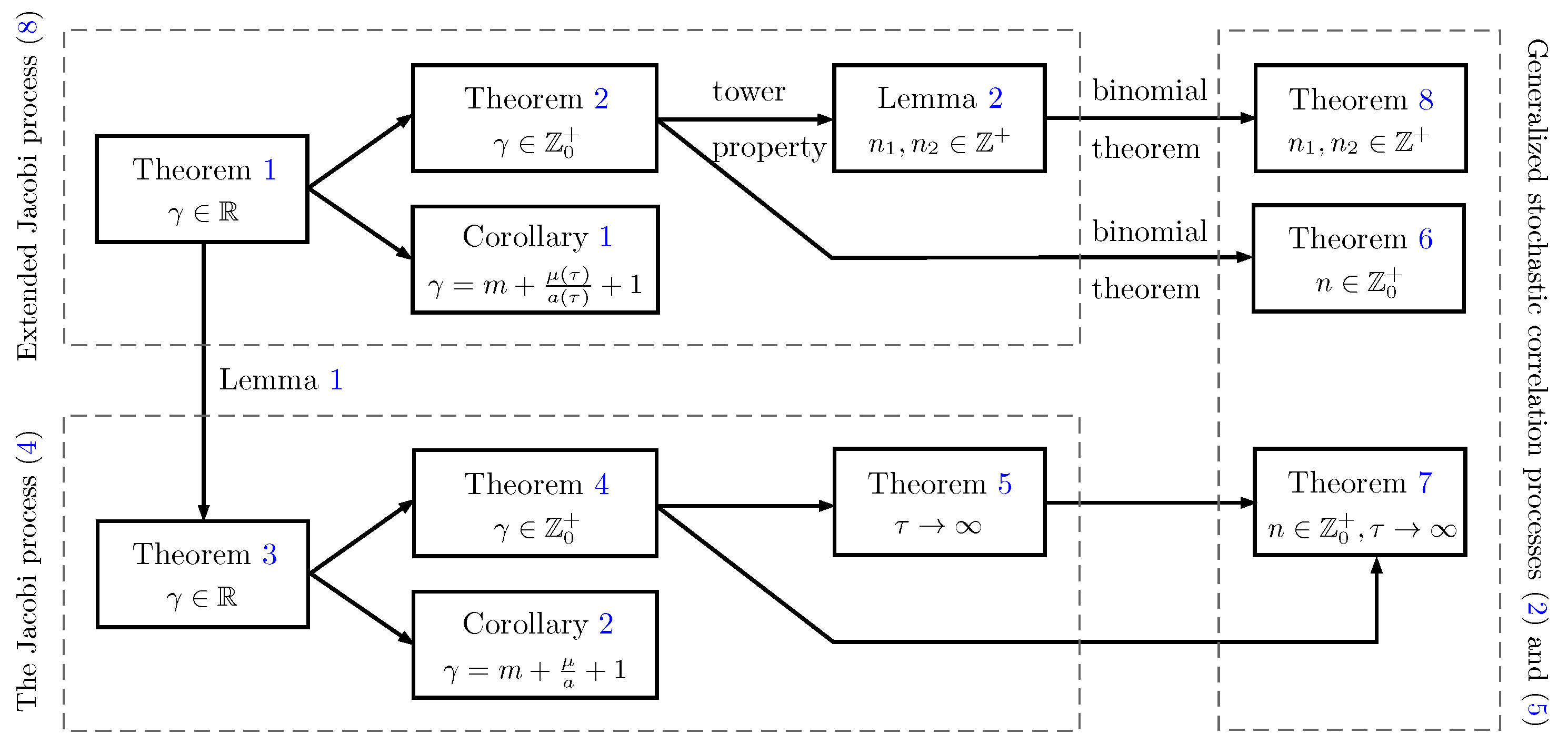
Remark 3.

Applying the idea in the proofs of Lemma 2 and Theorem 8, the general formula for conditional mixed moments $\mathbb{E}\left[{\rho }_{T_1}^{n_1}{\rho }_{T_2}^{n_2}{\rho }_{T_3}^{n_3}\dots {\rho }_{T_k}^{n_k}\mid {\rho }_s=\rho \right]$, where $n_1,n_2,n_3,\dots ,n_k\in {\mathbb{Z}}_0^{+}$ and $0\le s<T_1\le T_2\le T_3\le \dots \le T_k$, can be directly obtained. The advantage of our formula for conditional mixed moments (8) is its simple closed form, which can be used in many applications, especially to estimate the functions of the powers of observed processes which appeared in Sørensen [24], Leonenko and Šuvak [25,26], and Avram et al. [27]. Moreover, in order to study the integrated Jacobi process, the conditional mixed moments need to be evaluated. However, their proposed formulas are very complicated; see Forman and Sørensen [4]. Thus, our results can be applied easily.

Before finishing this section, we summarize the relationship of the presented formulas in the form of the diagram displayed in Figure 3, which shows the development process of the formulas consisting of ten theorems and two lemmas, which are categorized as performed in processes (2), (4), (5) and (8).

3.3. Statistical Properties

The conditional variance of the generalized stochastic correlation process (27) can be expressed as

$$\mathrm{Var}\left[{\rho }_T\mid {\rho }_s=\rho \right]=\mathbb{E}\left[{\left({\rho }_T-\mathbb{E}\left[{\rho }_T\mid {\rho }_s\right]\right)}^2\mid {\rho }_t=\rho \right]=U_G^{\langle 2\rangle }(\rho ,T-s)-{\left(U_G^{\langle 1\rangle }(\rho ,T-s)\right)}^2,$$

where $U_G^{\langle \gamma \rangle }(\rho ,T-s)$ is defined in Theorem 6. Furthermore, the $n\mathrm{th}$ moment about the mean, that is, the $n\mathrm{th}$ central moment, can be expressed as

$$\begin{array}{c}\hfill {\mathbf{\mu }}_n:=\mathbb{E}\left[{\left({\rho }_T-\mathbb{E}\left[{\rho }_T\mid {\rho }_s\right]\right)}^n\mid {\rho }_s=\rho \right]=\sum _{k=0}^n\left(\genfrac{}{}{0pt}{}{n}{k}\right)\left(U_G^{\langle k\rangle }(\rho ,T-s)\right){\left(-U_G^{\langle 1\rangle }(\rho ,T-s)\right)}^{n-k}.\end{array}$$

Well-known instances for the central moment are the zero-th moment ${\mathbf{\mu }}_0=1$, the 1st central moment ${\mathbf{\mu }}_1=0$, the 2nd central moment ${\mathbf{\mu }}_2=\mathrm{Var}\left[{\rho }_T\mid {\rho }_s=\rho \right]$, called the conditional variance, and the third ${\mathbf{\mu }}_3$ and fourth ${\mathbf{\mu }}_4$, known as the skewness and kurtosis, respectively.

We now move our focus to the conditional covariance and correlation. By applying Theorem 8, for $0\le s<T_1\le T_2$ where $\tau =T_2-s$, ${\tau }_1=T_1-s$ and ${\tau }_2=T_2-T_1$ we have

$$\begin{array}{cc}\hfill \mathrm{Cov}\left[{\rho }_{T_1},{\rho }_{T_2}\mid {\rho }_s=\rho \right]& =\mathbb{E}\left[\left({\rho }_{T_1}-\mathbb{E}\left[{\rho }_{T_1}\mid {\rho }_s\right]\right)\left({\rho }_{T_2}-\mathbb{E}\left[{\rho }_{T_2}\mid {\rho }_s\right]\right)\mid {\rho }_s=\rho \right]\hfill \\ \hfill & =\mathbb{E}\left[{\rho }_{T_1}{\rho }_{T_2}\mid {\rho }_s=\rho \right]-\mathbb{E}\left[{\rho }_{T_1}\mid {\rho }_s=\rho \right]\mathbb{E}\left[{\rho }_{T_2}\mid {\rho }_s=\rho \right]\hfill \\ \hfill & =\sum _{k=0}^1\sum _{j=0}^{2-k}{P}_k^{\langle 1\rangle }\left({\tau }_2\right)P_j^{\langle 2-k\rangle }\left({\tau }_1\right){\rho }^{2-k-j}-U_G^{\langle 1\rangle }(\rho ,{\tau }_1)U_G^{\langle 1\rangle }(\rho ,{\tau }_2)\hfill \end{array}$$

and the conditional correlation of the generalized stochastic correlation process (27) is

$$\begin{array}{cc}\hfill \mathrm{Corr}\left[{\rho }_{T_1},{\rho }_{T_2}\mid {\rho }_s=\rho \right]& =\frac{\mathrm{Cov}\left[{\rho }_{T_1},{\rho }_{T_2}\mid {\rho }_s=\rho \right]}{\sqrt{\mathrm{Var}[{\rho }_{T_1}\mid {\rho }_t=\rho ]}\sqrt{\mathrm{Var}[{\rho }_{T_2}\mid {\rho }_s=\rho ]}}.\hfill \end{array}$$

It should be noted that the analytical formulas for the conditional covariance and correlation can be extended to the analytical of $\mathrm{Cov}\left[{\rho }_{T_1}^{n_1},{\rho }_{T_2}^{n_2}\mid {\rho }_s=\rho \right]$ and $\mathrm{Corr}\left[{\rho }_{T_1}^{n_1},{\rho }_{T_2}^{n_2}\mid {\rho }_s=\rho \right]$ where $n_1,n_2\in {\mathbb{Z}}^{+}$. Several of the related applications as estimator tools are mentioned in [24,25,26,27,28].

4. Experimental Validation

As our results proposed in Section 3 are mainly based on the extended Jacobi process (8), this experimental validation section discusses this process first. In this experiment, we applied the Euler–Maruyama (EM) discretization method with MC simulations to process (8). Let ${\widehat{X}}_t$ be a time-discretized approximation of $X_t$ that is generated on time interval $[0,T]$ into N steps, i.e., $0=t_0<t_1<t_2<\dots <t_N=T$. Then, the EM approximate is defined by

$${\widehat{X}}_{t_{i+1}}={\widehat{X}}_{t_i}+\theta \left(t_i\right)\left(\mu \left(t_i\right)-{\widehat{X}}_{t_i}\right)\Delta t+\sqrt{2a\left(t_i\right)\theta \left(t_i\right){\widehat{X}}_{t_i}\left({\widehat{X}}_{t_i}-1\right)}\sqrt{\Delta t}{Z}_{i+1},$$

(33)

where the initial value ${\widehat{X}}_{t_0}=X_{t_0}$, $\Delta t=t_{i+1}-t_i$ is the size of the time step and $Z_i$ is the standard normal random variable. We illustrate the validations of the 1st moment ($n=1$) of the formula (15) via the parameters studied by Ardian and Kumral [29] for the evolution of gold prices and interest rates. For the generalized stochastic correlation process (2), their estimated parameters are ${\theta }^{*}\left(t\right)=1.15$, ${\mu }^{*}\left(t\right)=0.17$ and ${\sigma }^{*}\left(t\right)=0.56$ with ${\rho }_{\min }=-1$ and ${\rho }_{\max }=1$. Thus, for the extended Jacobi process (8), those parameters correspond to $\theta \left(t\right)=1.15$, $\mu \left(t\right)=0.59$ and $a\left(t\right)=-0.14$ for $t\in [0,\tau ]$; note that these parameters are all constants. This then corresponds to the Jacobi process (4) as well, which can compute the 1st conditional moment using formula (24) directly. This work was implemented in MATLAB libraries available in GitHub repositories: https://github.com/TyMathAD/Conditional_Mixed_Moments accessed on 21 April 2022.

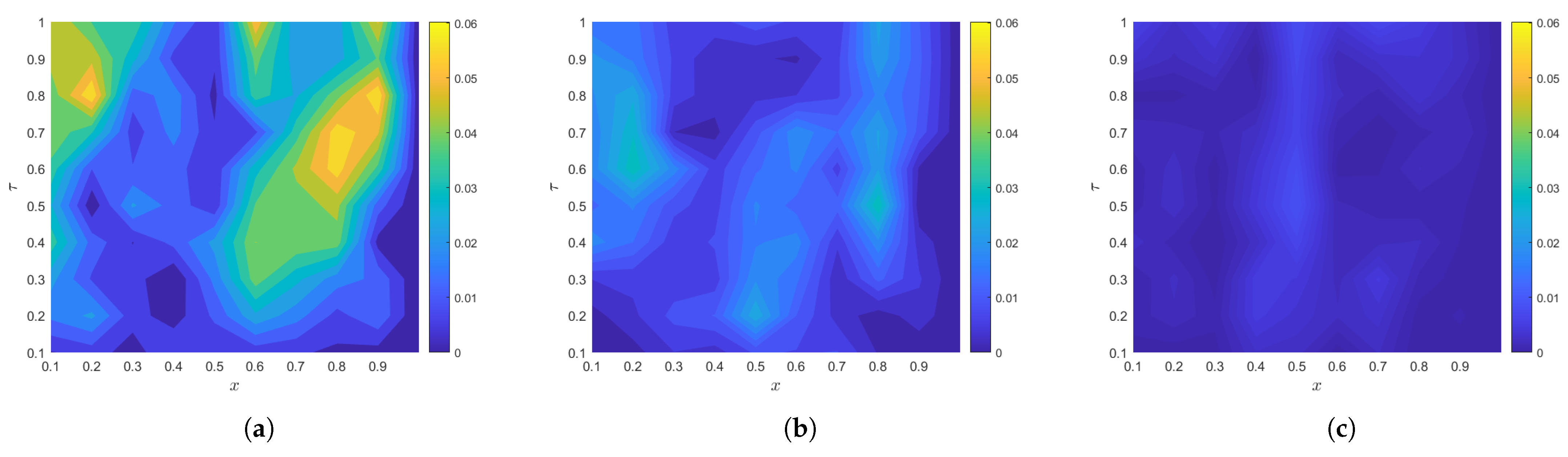
To test the efficiency of the 1st moment $U_J^{\langle 1\rangle }(x,\tau )$, we compared the obtained results with MC simulations at various points $(x,\tau )$, where $x,\tau \in \{0.1,0.2,0.3,\dots ,1\}$. These simulations were examined with the time step $\Delta t=0.0001$ and varied with the sample paths by 100, 1000, and 10,000, as depicted in Figure 4, which is the contour plotting of absolute errors between our formula and MC simulations. From Figure 4, we can see obviously that the contour colors trend to the dark blue shade for the larger path numbers. This means that the absolute errors approach zero. Figure 4a–c produces average absolute errors equal to $1.77\times {10}^{-2}$, $5.67\times {10}^{-3}$ and $6.42\times {10}^{-4}$, respectively. Hence, the MC simulations are most likely to converge to our formula.

In this validation, these obtained results of our formula and the MC simulations based on the EM method (33) were computed by implementing MATLAB R2021a software run on a laptop computer configured with the following details: Intel(R) Core(TM) i7-5700HQ, CPU @2.70 GHz, 16.0 GB RAM, Windows 10, 64-bit Operating System. As a result, the computational run time of our analytical formula is around 0.0145 s, while the MC simulations consume run times of 1.43, 4.32, and 40.21 s for 100, 1000, and 10,000 sample paths, respectively. Thus, we can see that the times of MC simulations are more tremendously expensive than our formula, especially, with large path numbers. It is notable that the MC simulations with just 100 paths spent more computing time than our formula, with almost 100 times the time elapsed. Hence, for a more accurate result the use of MC simulations may not be a good choice in terms of computing time. In contrast, the proposed formula is independent of any discretizations and has a very low computational cost. Therefore, the formulas presented here are efficient and suitable for practical use.

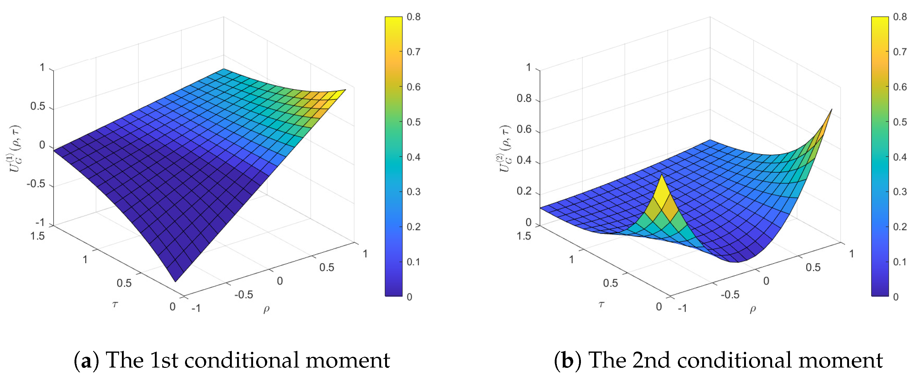
Moreover, we used the above parameters to compute the 1st and 2nd conditional moments, $U_G^{\langle 1\rangle }(\rho ,\tau )$ and $U_G^{\langle 2\rangle }(\rho ,\tau )$, in order to model the correlation between gold prices and interest rates. We computed these moments utilizing the presented formula (28) at different values $(\rho ,\tau )\in [-1,1]\times [0,1.5]$. 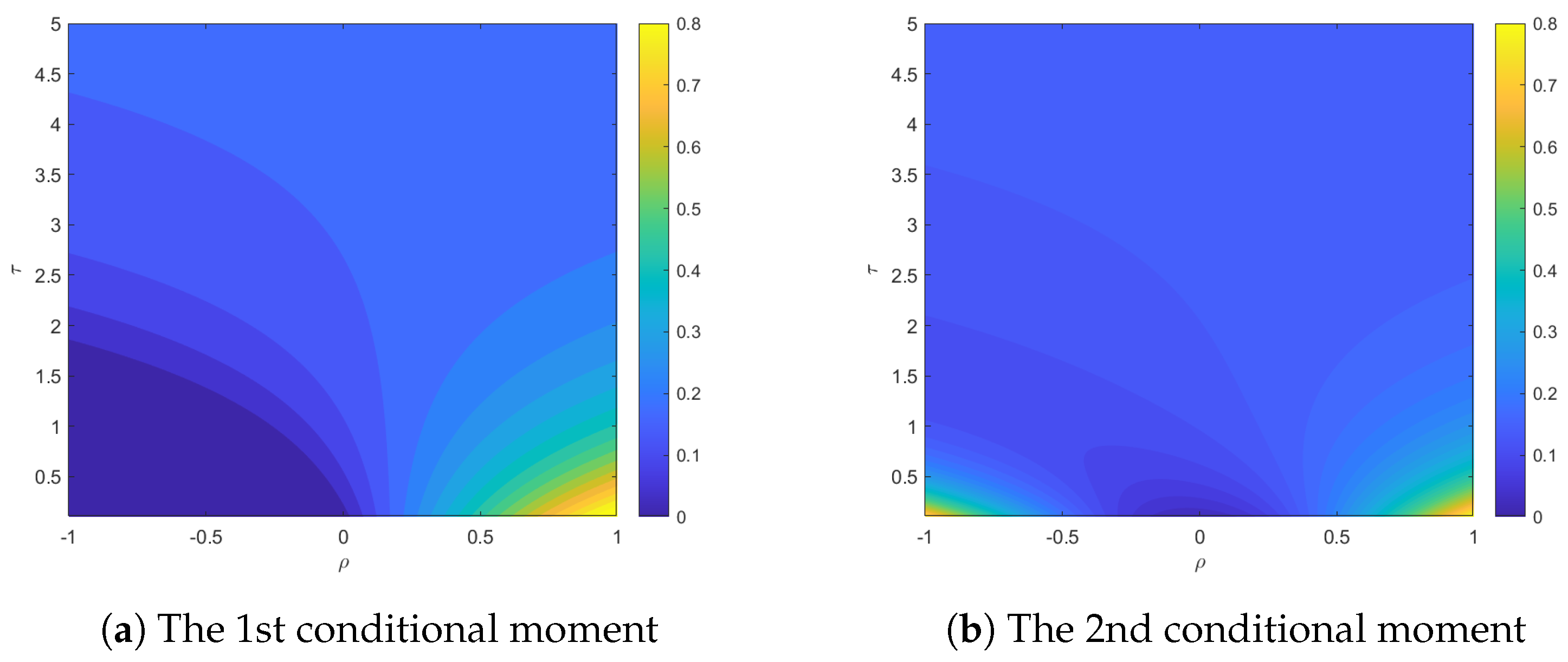The obtained results are demonstrated by surface plots in Figure 5. In addition, we plotted the graphical contours of the 1st and 2nd conditional moments for $(\rho ,\tau )\in [-1,1]\times [0,5]$. It can be seen that when $\tau$ is increasing, the obtained results converge to a certain value for both moments. This can be seen from Figure 6, in that the contour colors trend to a light blue shade which has an approximate value of $0.1$. Using Theorem 7, it is confirmed that when $\tau \to \infty$ these 1st and 2nd conditional moments are $0.17$ and $0.15$, respectively, corresponding to Figure 6.

Note that one primary concern for our proposed formula in Theorem 1 is that the coefficients $P_k^{\langle \gamma \rangle }\left(\tau \right)$ for $k\in {\mathbb{Z}}_0^{+}$ in (10) may not be exactly integrable. Thus, numerical integration methods are needed to manipulate the integral terms, such as a trapezoidal rule, Simpson’s rule, etc. One efficient method that we suggest to handle these integral terms is the Chebyshev integration method provided by Boonklurb et al. [30,31,32,33], which provides higher accuracy than other integration methods under the same discretization.

5. Method of Moments Estimator

In certain cases, the MM is superseded by Fisher’s method when estimating parameters of a known family of probability distribution, as the MLEs have a higher probability of being suitable to the quantities to be estimated. However, in certain cases such as the examples of gamma and beta distributions, MLEs may be intractable without computer programming. In this case, estimation using MM can be used as a first approximation of the solutions of the MLEs; the MM and the method of MLEs are symbiotic in this respect.

The key idea of the MM is to calibrate a well set of parameter values based on suitable conditional moments. In this section, suppose that we need to calibrate an unknown parameter vector $\mathsf{\theta }=\left({\theta }^{*},{\mu }^{*},{\sigma }^{*}\right)\in {\mathbb{R}}^3$ of the generalized stochastic correlation process (2), where the value of the true parameters is the vector ${\mathsf{\theta }}_0$ on discretely observed data ${\left\{{\rho }_{t_i}\right\}}_{1\le i\le n}$, where $t_{i-1}<t_i$ for all $i\in \{1,2,3,\dots ,n\}$. Normally, the basic conditional moments selected for calibration may be the first three conditional moments of the form provided in Theorem 6. It is sufficient to solve the unknown vector $\mathsf{\theta }$; however, in 2004, Gouriéroux and Valéry [3] suggested that we need to choose those conditional moments satisfying the identities of observed interest data.

They further determined sufficient moments to be adequately informative, such as the 1st, 2nd, 3rd (skewness), and 4th (kurtosis) conditional moments and the mixed moments $\mathbb{E}\left[{\rho }_{t_i}{\rho }_{t_{i-1}}^2\mid {\rho }_{t_0}=\rho \right]$ and $\mathbb{E}\left[{\rho }_{t_i}^2{\rho }_{t_{i-1}}^2\mid {\rho }_{t_0}=\rho \right]$ to capture the dynamics of the risk premium and the possible volatility persistence, respectively. Their set of conditional moments selected for implementing MM is

$$f\left({\rho }_{t_i},\mathsf{\theta }\right)=\left(\begin{array}{c}\begin{array}{cc}\hfill {\rho }_{t_i}-& \mathbb{E}\left[{\rho }_{t_i}\mid {\rho }_{t_0}=\rho \right]\hfill \\ \hfill {\rho }_{t_i}{\rho }_{t_{i-1}}-& \mathbb{E}\left[{\rho }_{t_i}{\rho }_{t_{i-1}}\mid {\rho }_{t_0}=\rho \right]\hfill \\ \hfill {\rho }_{t_i}^2-& \mathbb{E}\left[{\rho }_{t_i}^2\mid {\rho }_{t_0}=\rho \right]\hfill \\ \hfill {\rho }_{t_i}{\rho }_{t_{i-1}}^2-& \mathbb{E}\left[{\rho }_{t_i}{\rho }_{t_{i-1}}^2\mid {\rho }_{t_0}=\rho \right]\hfill \\ \hfill {\rho }_{t_i}^2{\rho }_{t_{i-1}}-& \mathbb{E}\left[{\rho }_{t_i}^2{\rho }_{t_{i-1}}\mid {\rho }_{t_0}=\rho \right]\hfill \\ \hfill {\rho }_{t_i}^2{\rho }_{t_{i-1}}^2-& \mathbb{E}\left[{\rho }_{t_i}^2{\rho }_{t_{i-1}}^2\mid {\rho }_{t_0}=\rho \right]\hfill \\ \hfill {\rho }_{t_i}^3-& \mathbb{E}\left[{\rho }_{t_i}^3\mid {\rho }_{t_0}=\rho \right]\hfill \\ \hfill {\rho }_{t_i}^4-& \mathbb{E}\left[{\rho }_{t_i}^4\mid {\rho }_{t_0}=\rho \right]\hfill \end{array}\end{array}\right),$$

with the conditional moments and mixed moments appearing above having been proposed in Theorems 6 and 8, respectively. In order to estimate parameters, we suppose that the conditional expectations of $f({\rho }_{t_i},\mathsf{\theta })$, $\mathbb{E}\left[f\left({\rho }_{t_i},\mathsf{\theta }\right)\mid {\mathcal{F}}_t\right]$, exist as a real number for all $i\in \{1,2,3,\dots ,n\}$, satisfying $\mathbb{E}\left[f\left({\rho }_{t_i},{\mathsf{\theta }}_0\right)\mid {\mathcal{F}}_t\right]=0$, and let

$${\mathbf{f}}_n\left(\mathsf{\theta }\right)=\frac{1}{n}\sum _{i=1}^{n}f\left({\rho }_i,\mathsf{\theta }\right).$$

The MM estimator of ${\mathsf{\theta }}_0$ based on the conditional expectation $\mathbb{E}\left[f\left({\rho }_{t_i},\mathsf{\theta }\right)\mid {\mathcal{F}}_t\right]$ is the solution to the system of equations ${\mathbf{f}}_n\left(\mathsf{\theta }\right)=0$. If we cannot solve the exact value of $\mathsf{\theta }$, a good estimate of the true value ${\mathsf{\theta }}_0$, called $\widehat{\mathsf{\theta }}$, is needed. In other words, we need a $\widehat{\mathsf{\theta }}$ that makes ${\mathbf{f}}_n\left(\widehat{\mathsf{\theta }}\right)$ close to 0; see more details in [34]. In any event, the algorithm that we suggest would use either Newton’s method or iterative methods to solve the system of nonlinear equations ${\mathbf{f}}_n\left(\widehat{\mathsf{\theta }}\right)=0$.

It should be noted that in certain cases, infrequent with large sample sizes and not as infrequent with small ones, the estimates provided by the MM are not suitable. In this case, they may be outside of the parameter space and it does not make sense to rely on the sample provided by the MM. In the context of the properties of the MM and its generalized version, under sufficient conditions they are consistent and asymptotically normally distributed; see for more details in [34,35].

6. Conclusions

Without the knowledge of the transition PDF, this paper presents a simple and novel approach for obtaining the analytical formulas for conditional moments and mixed moments of the extended Jacobi process. Those analytical formulas become concise forms under the Jacobi process. In addition, the analytical formulas for the unconditional moments are provided. By applying Ito’s lemma to the extended Jacobi process we obtain the generalized stochastic correlation process, and its analytic formulas for conditional moments are proposed. Statistical properties, namely, conditional variance, central moment, covariance, and correlation, are formulated. The validation of our formulas is shown by comparing the results with MC simulations. Our results can be used to find the parameters of correlation processes between financial product prices. Our study provides additional support for the work of those who require statistical tools to studying data governed by generalized stochastic correlation processes. Finally, a tool for estimating parameters concerning the calculation of moments is provided as well.