
Unified Integrals of Generalized Mittag–Leffler Functions and Their Graphical Numerical Investigation

 ,
,  and
and 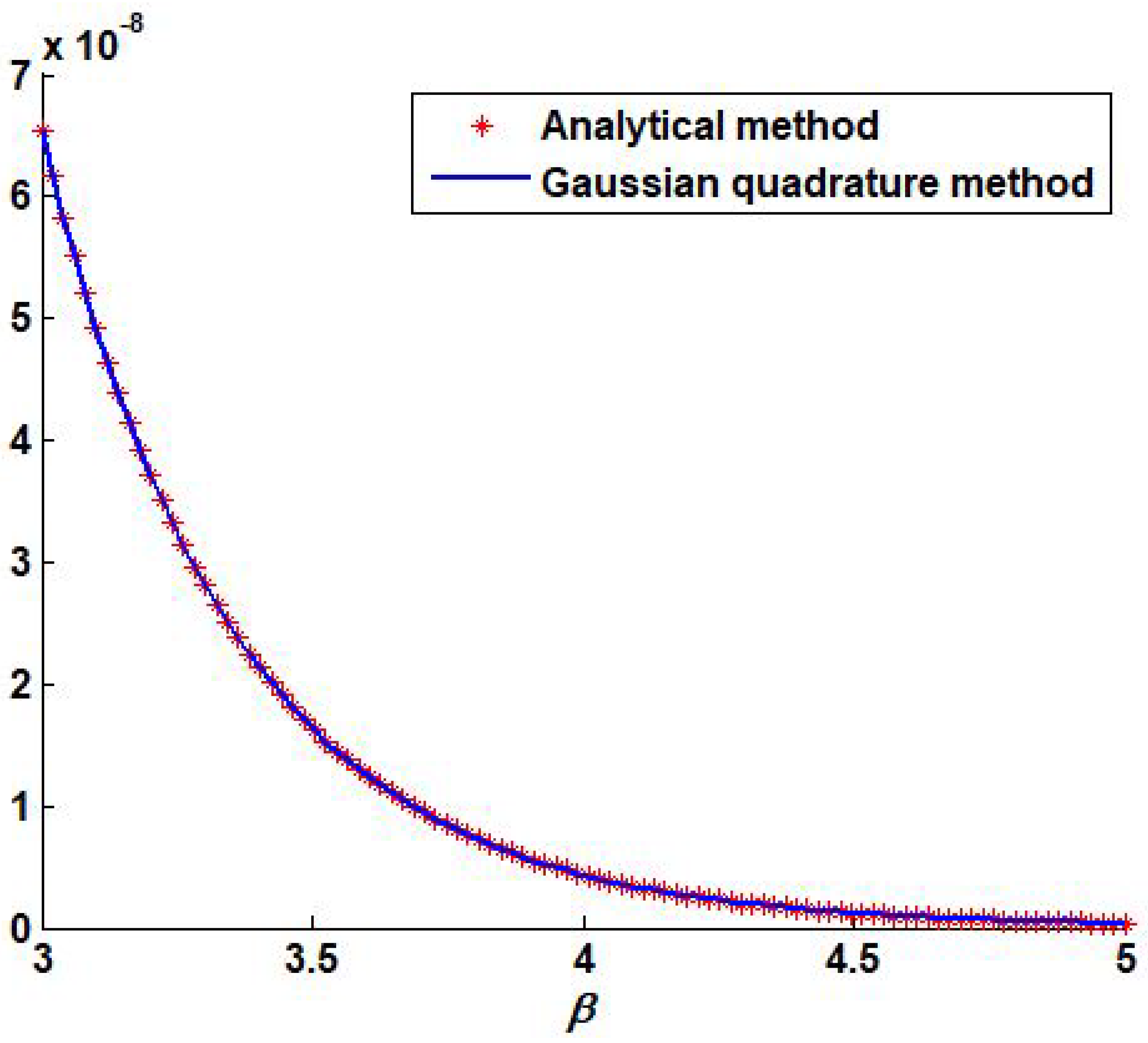
Abstract
:1. Introduction
2. Main Results
3. Special Cases
- (i)
- On setting = , = in (15), the following identity holds:
- (ii)
- Setting = , = and in (15), the following identity holds:
- (iii)
- Setting = , = and in (15), the following identity holds:
- (iv)
- Setting = , = and in (15), the following identity holds:
- (v)
- Setting = , = and in (15), the following identity holds:
- (vi)
- Setting = , = and in (15), the following identity holds:
- (vii)
- Setting = , = and in (15), the following identity holds:
- (viii)
- Setting = , = and in (15), the following identity holds:
- (ix)
- Setting = , = and , in (15), the following identity holds:
- (x)
- Setting = , = in (20), the following identity holds:
- (xi)
- Setting = , = and in (20), the following identity holds:
- (xii)
- Setting = , = and in (20), the following identity holds:
- (xiii)
- Setting = , = and in (20), the following identity holds:
- (xiv)
- Setting = , = and in (20), the following identity holds:
- (xv)
- Setting = , = and in (20), the following identity holds:
- (xvi)
- Setting = , = and in (20), the following identity holds:
- (xvii)
- Setting = , = and in (20), the following identity holds:
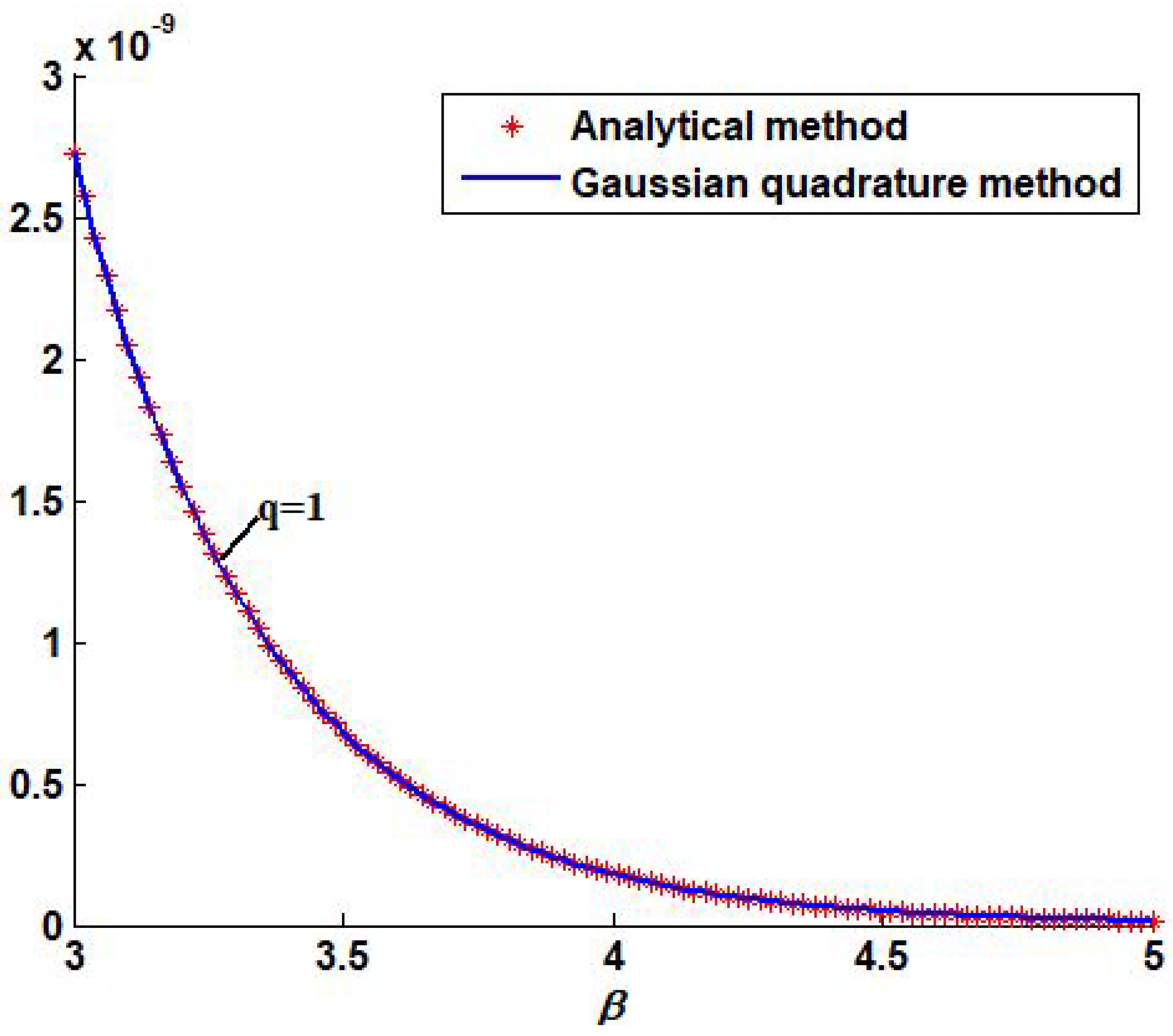
4. Graphical Representation
5. Conclusions
Author Contributions
Funding
Institutional Review Board Statement
Informed Consent Statement
Data Availability Statement
Acknowledgments
Conflicts of Interest
References
- Jain, S.; Agarwal, P.; Ahmad, B.; Al-Omari, S. Certain recent fractional integral inequalities associated with the hypergeometric operators. J. King Saud Univ.-Sci. 2016, 28, 82–86. [Google Scholar] [CrossRef] [Green Version]
- Al-Omari, S.; Baleanu, D. On the Generalized Stieltjes transform of Fox’s kernel function and its properties in the space of generalized functions. J. Comput. Anal. Appl. 2017, 23, 108–118. [Google Scholar]
- Agarwal, P.; Jain, S.; Kıymaz, I.O.; Chand, M.; Al-Omari, S. Certain sequence of functions involving generalized hypergeometric functions. Math. Sci. Appl. E-Notes 2015, 3, 45–53. [Google Scholar] [CrossRef]
- Khan, N.; Usman, T.; Aman, M.; Al-Omari, S.; Choi, J. Integral transforms and probality distributions involving generalized hypergeometric function. Georgian J. Math. 2021, 28, 2021–2105. [Google Scholar] [CrossRef]
- Chandak, S.; Al-Omari, S.K.Q.; Suthar, D.L. Unified integral associated with the generalized V-function. Adv. Differ. Equ. 2020, 2020, 560. [Google Scholar] [CrossRef]
- Choi, J.; Agarwal, P. A note on generalized integral operator associated with multiindex Mittag-Leffler function, Filomat 30, 1931–1939. Adv. Differ. Equ. 2020, 448, 1–11. [Google Scholar] [CrossRef]
- Gorenflo, R.; Kilbas, A.A.; Mainardi, F.; Rogosin, S.V. Mittag-Leffler Functions, Related Topics and Applications; Springer: New York, NY, USA, 2020; p. 540. [Google Scholar]
- Haubold, H.J.; Mathai, A.M.; Saxena, R.K. Mittag-Leffler Functions and Their Applications. J. Appl. Math. 2011, 2011, 298628. [Google Scholar] [CrossRef] [Green Version]
- Kiryakova, V. Generalized Fractional Calculus and Applications; CRC Press: Boca Raton, FL, USA, 1993. [Google Scholar]
- Kiryakova, V. The multi-index Mittag-Leffler functions as an important class of special functions of fractional calculus. Comput. Math. Appl. 2010, 59, 1885–1895. [Google Scholar] [CrossRef] [Green Version]
- Kochubei, A.; Luchko, Y. Fractional Differential Equations. In Handbook of Fractional Calculus with Applications; De Gruyter: Berlin, Germany, 2019; Volume 2. [Google Scholar]
- Mainardi, F. Why the Mittag-Leffler Function Can Be Considered the Queen Function of the Fractional Calculus? Entropy 2020, 22, 1359. [Google Scholar] [CrossRef] [PubMed]
- Agarwal, P.; Choi, J.; Jain, S.; Rashidi, M.M. Certain integrals associated with generalized mittag-leffler function. Commun. Korean Math. Soc. 2017, 32, 29–38. [Google Scholar] [CrossRef] [Green Version]
- Almalahi, M.A.; Ghanim, F.; Botmart, T.; Bazighifan, O.; Askar, S. Qualitative Analysis of Langevin Integro-Fractional Differential Equation under Mittag–Leffler Functions Power Law. Fractal Fract. 2021, 5, 266. [Google Scholar] [CrossRef]
- Kamarujjama, M.; Khan, N.; Khan, O. Estimation of certain integrals with extended multi-index Bessel function. Malaya J. Mat. 2019, 7, 206–212. [Google Scholar] [CrossRef] [Green Version]
- Khan, N.; Usman, T.; Aman, M.; Al-Omari, S.; Araci, S. Computation of certain integral formulas involving generalized Wright function. Adv. Differ. Equ. 2020, 2020, 491. [Google Scholar] [CrossRef]
- Khan, N.; Usman, T.; Aman, M. Some properties concerning the analysis of generalized Wright function. J. Comput. Appl. Math. 2020, 376, 112840. [Google Scholar] [CrossRef]
- Khan, N.; Khan, S. Integral transform of generalized K-Mittag-Lefller function. J. Fract. Calc. Appl. 2018, 9, 13–21. [Google Scholar]
- Khan, N.; Ghayasuddin, M.; Shadab, M. Some Generating Relations of Extended Mittag-Leffler Functions. Kyungpook Math. J. 2019, 59, 325–333. [Google Scholar]
- Khan, N.; Husain, S. A note on extended beta function involving generalized Mittag-Leffler function and its applications. TWMS J. App. Eng. Math. 2022, 12, 71–81. [Google Scholar]
- Khan, O.; Khan, N.; Sooppy, K.A. Unified approach to the certain integrals of k-Mittag-Leffler type function of two variables. Trans. Natl. Acad. Sci. Azerb. Ser. Phys.-Tech. Math. Sci. Math. 2019, 39, 98–108. [Google Scholar]
- Mihai, M.V.; Awan, M.U.; Noor, M.A.; Du, T.; Kashuri, A.; Noor, K.I. On Extended General Mittag–Leffler Functions and Certain Inequalities. Fractal Fract. 2019, 3, 32. [Google Scholar] [CrossRef] [Green Version]
- Prabhakar, T.R. A Singular Integral Equation with a Generalized Mittag-Leffler Function in the Kernel. Yokohama Math. J. 1971, 19, 7–15. [Google Scholar]
- Prudnikov, A.P.; Brychkov, Y.A.; Marichev, O.I. Integral and Series V.1. More Special Functio; Gordon and Breach: New York, NY, USA; London, UK, 1992. [Google Scholar]
- Rainville, E.D. Special Functions; The Macmillan Company: New York, NY, USA, 1960. [Google Scholar]
- Salim, T.O. Some properties relating to the generalized Mittag-Leffler function. Adv. Appl. Math. Anal. 2009, 4, 21–30. [Google Scholar]
- Salim, T.O.; Faraj, A.W. A generalization of Mittag-Leffler function and integral operator associated with fractional calculus. J. Fract. Calc. Appl. 2012, 3, 1–13. [Google Scholar]
- Shukla, A.; Prajapati, J. On a generalization of Mittag-Leffler function and its properties. J. Math. Anal. Appl. 2007, 336, 797–811. [Google Scholar] [CrossRef] [Green Version]
- Singh, P.; Jain, S.; Cattani, C. Some Unified Integrals for Generalized Mittag-Leffler Functions. Axioms 2021, 10, 261. [Google Scholar] [CrossRef]
- Suthar, D.L.; Amsalu, H.; Godifey, K. Certain integrals involving multivariate Mittag-Leffler function. J. Inequalities Appl. 2019, 2019, 208–224. [Google Scholar] [CrossRef] [Green Version]
- Mittag-Leffler, G.M. Sur la nouvelle fonction Eα(x). CR Acad. Sci. Paris 1903, 137, 554–558. [Google Scholar]
- Rahman, G.; Suwan, I.; Nisar, K.S.; Abdeljawad, T.; Samraiz, M.; Ali, A. A basic study of a fractional integral operator with extended Mittag-Leffler kernel. AIMS Math. 2021, 6, 12757–12770. [Google Scholar] [CrossRef]
- Wiman, A. Uber den fundamental Satz in der Theories der Funktionen Eα(z). Acta Math. 1905, 29, 191–201. [Google Scholar] [CrossRef]
- Khan, M.A.; Ahmed, S. On some properties of the generalized Mittag-Leffler function. SpringerPlus 2013, 2, 337. [Google Scholar] [CrossRef] [PubMed] [Green Version]
- Wright, E.M. The asymptotic expansion of integral functions defined by Taylor series. Philos. Trans. R. Soc. London. Ser. A Math. Phys. Sci. 1940, 238, 423–451. [Google Scholar] [CrossRef]
- Al-Omari, S. Estimation of a modified integral associated with a special function kernel of Fox’s H-function type. Commun. Korean Math. Soc. 2020, 35, 125–136. [Google Scholar]
- Abramowitz, M.; Stegun, I.A. (Eds.) Handbook of Mathematical Functions with Formulas, Graphs, and Mathematical Tables; US Government Printing Office: Washington, DC, USA, 1948; Volume 55.
- Fox, C. The Asymptotic Expansion of Generalized Hypergeometric Functions. Proc. Lond. Math. Soc. 1928, 2, 389–400. [Google Scholar] [CrossRef]
- Al-Omari, S. A revised version of the generalized Krätzel-Fox integral operators. Mathematics 2018, 6, 222. [Google Scholar] [CrossRef] [Green Version]
- Al-Omari, S. On a Class of Generalized Meijer-Laplace Transforms of Fox Function Type Kernels and Their Extension to a Class of Boehmians. Georgian Math. J. 2018, 25, 1–8. [Google Scholar] [CrossRef]
- Wright, E.M. The asymptotic expansion of the generalized hypergeometric function. Proc. Lond. Math. Soc. 1940, 2, 389–408. [Google Scholar] [CrossRef]
- Wright, E.M. The asymptotic expansion of the generalized hypergeometric function. J. Lond. Math. Soc. 1935, 1, 286–293. [Google Scholar] [CrossRef]


Publisher’s Note: MDPI stays neutral with regard to jurisdictional claims in published maps and institutional affiliations. |
© 2022 by the authors. Licensee MDPI, Basel, Switzerland. This article is an open access article distributed under the terms and conditions of the Creative Commons Attribution (CC BY) license (https://creativecommons.org/licenses/by/4.0/).
Share and Cite
Khan, N.; Khan, M.I.; Usman, T.; Nonlaopon, K.; Al-Omari, S. Unified Integrals of Generalized Mittag–Leffler Functions and Their Graphical Numerical Investigation. Symmetry 2022, 14, 869. https://doi.org/10.3390/sym14050869
Khan N, Khan MI, Usman T, Nonlaopon K, Al-Omari S. Unified Integrals of Generalized Mittag–Leffler Functions and Their Graphical Numerical Investigation. Symmetry. 2022; 14(5):869. https://doi.org/10.3390/sym14050869
Chicago/Turabian StyleKhan, Nabiullah, Mohammad Iqbal Khan, Talha Usman, Kamsing Nonlaopon, and Shrideh Al-Omari. 2022. "Unified Integrals of Generalized Mittag–Leffler Functions and Their Graphical Numerical Investigation" Symmetry 14, no. 5: 869. https://doi.org/10.3390/sym14050869