Determining Ground-State Phase Diagrams on Quantum Computers via a Generalized Application of Adiabatic State Preparation

Abstract

Quantum phase transitions materialize as level crossings in the ground-state energy when the parameters of the Hamiltonian are varied. The resulting ground-state phase diagrams are straightforward to determine by exact diagonalization on classical computers, but are challenging on quantum computers because of the accuracy needed and the near degeneracy of the competing states close to the level crossings. On the other hand, classical computers are limited to small system sizes, which quantum computers may help overcome. In this work, we use a local adiabatic ramp for state preparation to allow us to directly compute ground-state phase diagrams on a quantum computer via time evolution. This methodology is illustrated by examining the ground states of the XY model with a magnetic field in the z-direction in one dimension. We are able to calculate an accurate phase diagram on both two- and three-site systems using IBM quantum machines.

1. Introduction

Quantum computers are thought to enable calculations that cannot be carried out on classical computers [1,2,3,4,5]. For simulating quantum systems, classical computers are limited to exact diagonalization as there are no good approximation methods available in general. However, exact diagonalization cannot be employed in large systems, as the Hilbert space grows exponentially with respect to the system size [3]. One challenging problem in many-body physics is to determine the zero-temperature phase diagram of finite systems that have level crossings in the ground state as the parameters in the Hamiltonian are tuned across the transition [6,7]. Such phase diagrams commonly occur when a system has competing order parameters [8]. One possible approach to solving this problem is to simply create circuits for target wave functions that can have their parameters varied to allow for a variational determination of the approximate ground state. Then, one can determine the phase diagram by examining the quantum numbers and the symmetries of the variational wave function. However, such an approach is likely to fail or to be inaccurate; this is because there are low-lying states near the level crossings and the variational calculations need to be done with high accuracy to carry out such a program. This becomes especially complicated if the variational state ansatz does not belong to the subspace corresponding to the ground-state quantum numbers.

Another approach one could try is to use adiabatic state preparation: start the system in an easy to prepare state that is the ground state of the Hamiltonian for a given parameter, and then slowly change the parameters in the Hamiltonian. If we change slowly enough, the adiabatic theorem guarantees that we stay in the ground state. This approach may also have problems, because the time evolution will preserve the symmetry of the wave function, and level crossings can only occur between states with different symmetries.

However, we can modify the adiabatic state preparation protocol by adding a small symmetry-breaking field, and we can find the phase transition point by monitoring the expectation value of the quantum numbers corresponding to the different symmetries on either side of the phase transition. Now, because the symmetries are only approximate, a sufficiently slow time evolution will map out the ground-state phase diagram. We then repeat with different magnitudes of the symmetry-breaking field and extrapolate the results to the limit where the symmetry-breaking field vanishes. In this fashion, we can employ adiabatic state preparation to carry out a mapping of the ground-state phase diagram. It is unlikely that fast forwarding techniques such as QAOA [9] or shortcuts to adiabaticity [10,11], will help with carrying out this approach because it may require very accurate optimization near the level crossing, or knowledge of the eigenstates or invariants of motion, which maybe costly to find.

We test our approach on the ground-state phase diagram of an isotropic 1D XY model in a magnetic field along the z-direction. This system is a stringent test for such an approach, because there are N phase transitions for an N-site system in the region where $|B_z|\le |J|$. As the system size is made larger, the problem becomes increasingly more challenging to solve. In fact, the model may exhibit a devil’s staircase in the ground-state phase diagram [12]. The conserved symmetry (quantum number) is the z-component of total spin, so we can monitor the phase diagram by measuring the magnetization of the system.

Our strategy is to start the system in a large $B_z$ field, and to add a small symmetry-breaking field $B_x$ in a perpendicular direction. The initial state will be taken to be polarized along the z-direction, which is easy to prepare. We ramp the z-field down, keeping the x-field fixed, using a local adiabatic ramp [13]. This approach was originally used to generate the ground state of the transverse-field Ising model in ion-trap quantum simulators. For the two-site system, we also performed the experiment starting from all spins aligned down and ramping up the $B_z$ field. We find that for two- and three-site systems, this approach gives accurate phase diagrams in IBM quantum machines.

2. Materials and Methods

We work with the one-dimensional isotropic XY model with periodic boundary conditions and a magnetic field along the z direction, as shown in Equation (1) for a system with L spins:

$$H=-\sum _{i=1}^L\left[\frac{J}{4}\left({\sigma }_i^x{\sigma }_{i+1}^x+{\sigma }_i^y{\sigma }_{i+1}^y\right)+\frac{B_z}{2}{\sigma }_i^z\right].$$

(1)

where ${\sigma }_i^{x,y,z}$ are the usual Pauli matrices obtained by setting $(\hslash =1)$ in the spin operators of the ith site, $S_i^{x,y,z}=\frac{\hslash }{2}{\sigma }_i^{x,y,z}$. This model can be solved exactly by fermionization using a Jordan–Wigner (JW) transformation [14] and a subsequent Fourier transformation to momentum space [15]. The boundary term needs more care as it still has the JW string in it. Usually, for a large system this term is negligible. Alternatively, we simply consider the periodic term without a JW string attached, so that the usual Fourier transform yields the fermionic eigen energies. Then, the fermionic Hamiltonian takes the form

$$H=\sum _k\left({\omega }_k{c}_k^{†}{c}_k-\frac{B_z}{2}\right)$$

(2)

where ${\omega }_k=\left(-Jcosk+B_z\right)$ and $k=\frac{2n\pi }{L}$, with $n=-\frac{L}{2}+1,\cdots ,0,\cdots ,\frac{L}{2}$.

For a finite-size system the boundary term matters; this can be dealt with by making use of the fermionic parity [16]. The system is decoupled into odd and even parity sectors, where periodic and anti-periodic boundary terms emerge, respectively. This results in the same form for the fermionic Hamiltonian, but with different momenta for the different parity sectors. For odd parity sector, the momenta are the ones mentioned above (which includes the zero momentum point), whereas for an even parity sector, the momenta are shifted to $k=\pm \frac{(2n-1)\pi }{L}$, with $n=1,\cdots ,\frac{L}{2}$. One challenge with this approach is that each parity sector has $2^L$ eigenvalues while the exact solution (over both parities) has exactly $2^L$ eigenvalues. To avoid any of these issues, we work in the original spin representation throughout this paper.

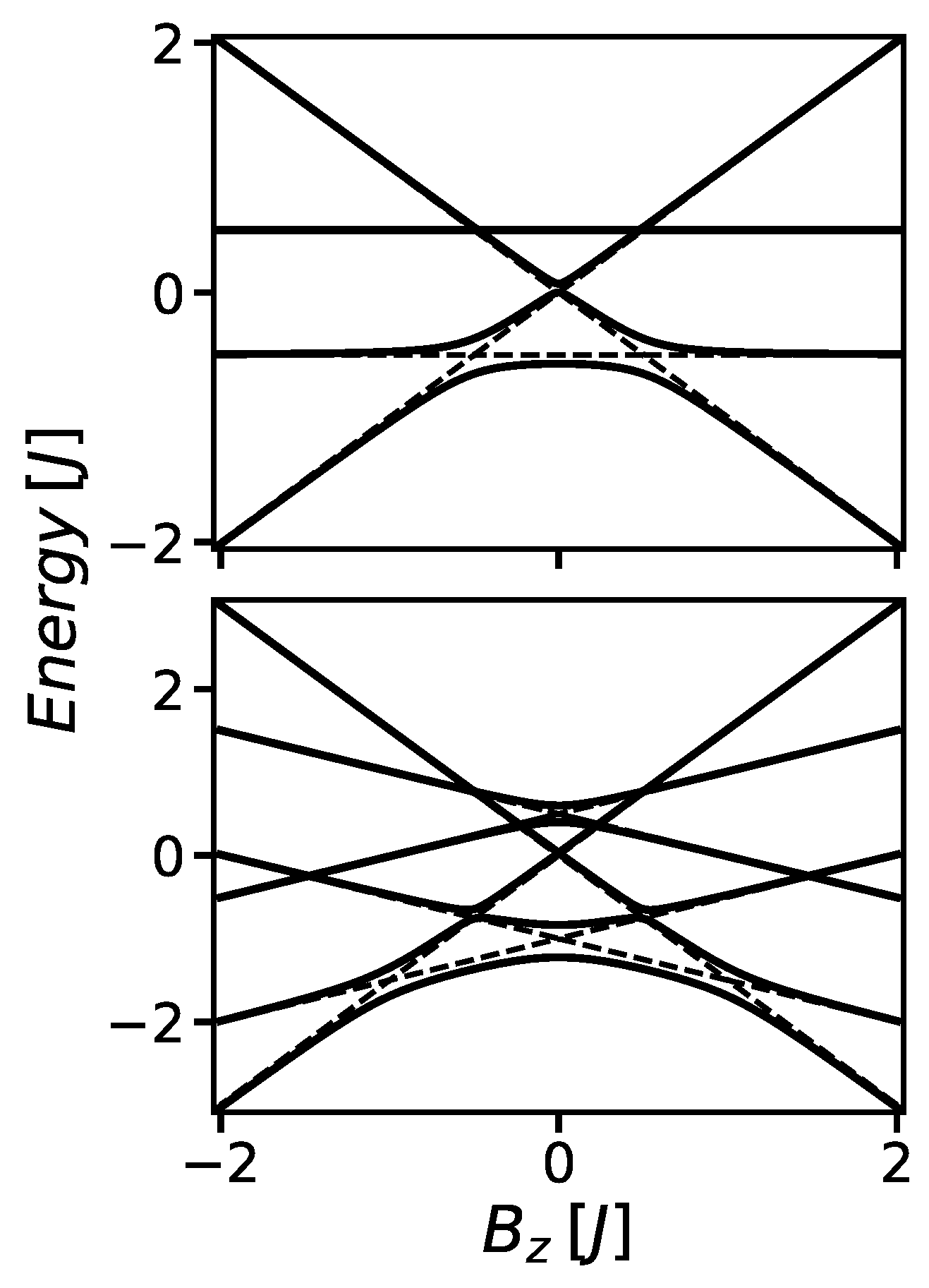
The ground state has many level crossings as a function of the magnetic field $B_z$. This is illustrated in Figure 1 and Figure 2. Figure 1 shows the expectation value of the z-component of spin (also known as the magnetization) as a function of $B_z$. Each of the vertical steps on the exact curve corresponds to a level crossing, where the quantum number for the z-component of spin shifts by one unit; the plot also shows an adiabatic-time evolution, which will be discussed later. In this work, we show how to obtain these quantum phase transition points (critical $B_z$ values) on a quantum computer.

In adiabatic-state preparation, we start from the ground state of a Hamiltonian, which is easy to prepare, and then we slowly evolve the state using time evolution with a Hamiltonian that interpolates from the initial Hamiltonian to the target Hamiltonian. The amount of diabatic excitations are determined by how fast the Hamiltonian changes near the avoided-crossing spectral gaps between the ground and excited states. The initial Hamiltonian can be thought of as a Hamiltonian with $J=0$, or equivalently with $B_z\gg J$. Then, the magnetic field is ramped down to a final value (e.g., zero) where ideally we end up in the ground state of the final Hamiltonian. However, this cannot occur if there is additional symmetry in the Hamiltonian. Here, because $S^z={\sum }_i{\sigma }_i^z/2$ commutes with H, we can simultaneously diagonalize both operators and this means the quantum number corresponding to the total z-component of spin (m) are unchanged during time evolution. Thus, we only stay in the ground state of a system with definite z-component of spin. This can be seen in Figure 2, where the dotted lines show a level crossing for a two- and three-site system.

In order to achieve adiabatic-state preparation, we must break the symmetry. We do so by adding a small $B_x$ field, upon which $[S_z,H]\ne 0$. This means states that used to have different m quantum numbers are now coupled together. This can be seen in Figure 2, where the solid lines show avoided level crossings for a two- and three-site system with a $B_x$ field. This then allows adiabatic-state preparation to take place, and if we go slow enough, we will have limited diabatic excitation out of the ground state. Figure 1 shows that with a $B_x$ field one can traverse through all the magnetization sectors in a 10-site system. However, the $B_x$ term changes the Hamiltonian and its energy levels. We only have quantum phase transitions when $B_x=0$, which implies we must extrapolate to the $B_x\to 0$ limit. With the $B_x$ term, the modified Hamiltonian is

$$H=-\sum _{i=1}^L\left[\frac{J}{4}\left({\sigma }_i^x{\sigma }_{i+1}^x+{\sigma }_i^y{\sigma }_{i+1}^y\right)+\frac{B_x}{2}{\sigma }_i^x+\frac{B_z}{2}{\sigma }_i^z\right].$$

(3)

The time evolution is implemented with a local adiabatic ramp [17,18], which is constructed to yield the same diabatic excitation for each time step of the time evolution. It does so by ramping faster when the gap to the first excited state is large and more slowly when the gap is small. It is determined by adjusting the rate $\frac{d{B}_z}{dt}$ according to the instantaneous energy gap $\mathsf{\Delta }\left(B_z\right)$ such that $|\frac{d{B}_z}{dt}|\ll {\mathsf{\Delta }}^2\left(B_z\right)$ [18]. This provides the highest fidelity ramp for a given total time of evolution.

The total time for the local ramp is determined by an adiabaticity parameter ($\gamma$). We require $\gamma \gg 1$ for an adiabatic ramp, where $\gamma =\frac{{\mathsf{\Delta }}^2\left(B_z\right)}{\left|d{B}_z\left(t\right)/dt\right|}$. Starting from a magnetic field $B_{z,\mathrm{initial}}$ and ramping down to a magnetic field $B_{z,\mathrm{final}}$ the ramp time t is given by

$$t=-\gamma {\int }_{B_{z,\mathrm{initial}}}^{B_{z,\mathrm{final}}}\frac{d{B}_z}{{\mathsf{\Delta }}^2\left(B_z\right)}.$$

(4)

where $\mathsf{\Delta }$ is the energy difference between first excited state and ground state and the minus sign indicates that we are ramping down. One can either choose the adiabaticity parameter first, and determine the total time, or one can fix the total time and infer the adiabaticity parameter. A resulting local adiabatic ramp for a two- and three-site system is shown in Figure 3. The ramp was implemented via a Trotter product formula. We selected the adiabaticity parameter and the number of Trotter steps such that we can accurately determine the different steps in the magnetization; the magnetization then signals the different regions of the ground-state-phase diagram. Specifically, we fixed $\gamma$ and increased the number of steps from a small number of total steps such that the magnetization switches to the next sector for all the $B_x$ values. The goal is to implement the ramp with a small total number of steps so that depth of the circuits implemented on the quantum computer is reduced.

The same strategy is used on a quantum computer. We use the first-order Trotter product formula for the time-evolution operator from $t_0$ to t:

$$\mathbf{U}\left(t,t_0\right)\approx e^{-i\mathbf{H}(t-dt)dt}{e}^{-i\mathbf{H}(t-2dt)dt}\dots e^{-i\mathbf{H}\left(t_0\right)dt}.$$

(5)

Then, each Trotter step further is decomposed into two qubit and single qubit gates so that it can be implemented on the IBM machines using their native gate set.

This procedure yields values for $dt$ that are larger than is typical for Trotter decomposition; for example, for the two-site system we obtain $dt=8.45/J$ for $B_x$ = $0.02J$ (see Figure 4). However, while the absolute value of $dt$ is large, it is ameliorated by two factors. First, the non-commuting part of the Hamiltonian is entirely proportional to $B_x$, which is small, so that the effective small parameter is really $dt{B}_x$. Second, the leading-order commutator arising from the Baker–Campbell–Hausdorff (BCH) expansion of the time evolution from $t_1$ to $t_2$ when $\frac{dt}{2}<1$ is further suppressed by the slowly varying magnetic field $B_z\left(t\right)$ as

$$\begin{array}{c}\hfill \left|\frac{[H\left(t_1\right)dt,H\left(t_2\right)dt]}{2}\right|=\left|\frac{d{t}^2{B}_x}{4}\left[B_z\left(t_2\right)-B_z\left(t_1\right)\right]\sum _{i=1}^N{\sigma }_i^y\right|\end{array}$$

(6)

Thus, as long $dB/dt$ is not too large, the error arising from Trotterization is manageable—this is expected because when the Hamiltonian is time independent, it commutes with itself at all times and no error arises from the BCH expansion. One additional source of Trotter error arises from the gate decomposition of the time evolution operator—here, the leading error is similarly proportional to $B_x{\left(\frac{dt}{2}\right)}^2$. This is the leading order in BCH expansion when $\frac{dt}{2}<1$, e.g., in our three-site experiments (see Figure 5). For two sites and three sites, we have confirmed empirically that the magnetization goes to the next sector with the given $dt$ (run on a simulator). The behavior of the crossing points for a 1000 Trotter step evolution is shown in Figure 6 and Figure 7. For larger systems, one might need to increase the number of Trotter steps so that $dt$ is small and follows the adiabatic evolution more closely.

The determination of the phase diagram then proceeds as follows: (i) we initialize the system in a state that is all up and with the magnetic field equal to $B_{z\mathrm{initial}}$ and with a fixed value for $B_x$; (ii) we evolve the system from $t_0$ to t using the local adiabatic ramp for $B_z\left(t\right)$; (iii) at each time step, we measure the magnetization; (iv) using the magnetization, we determine the critical value of $B_z$, which corresponds to the midpoint of the step in the magnetization between two successive m quantum numbers; (v) we repeat these steps for a different value of $B_x$; and (vi) we extrapolate the critical $B_z$ field to the limit where $B_x\to 0$.

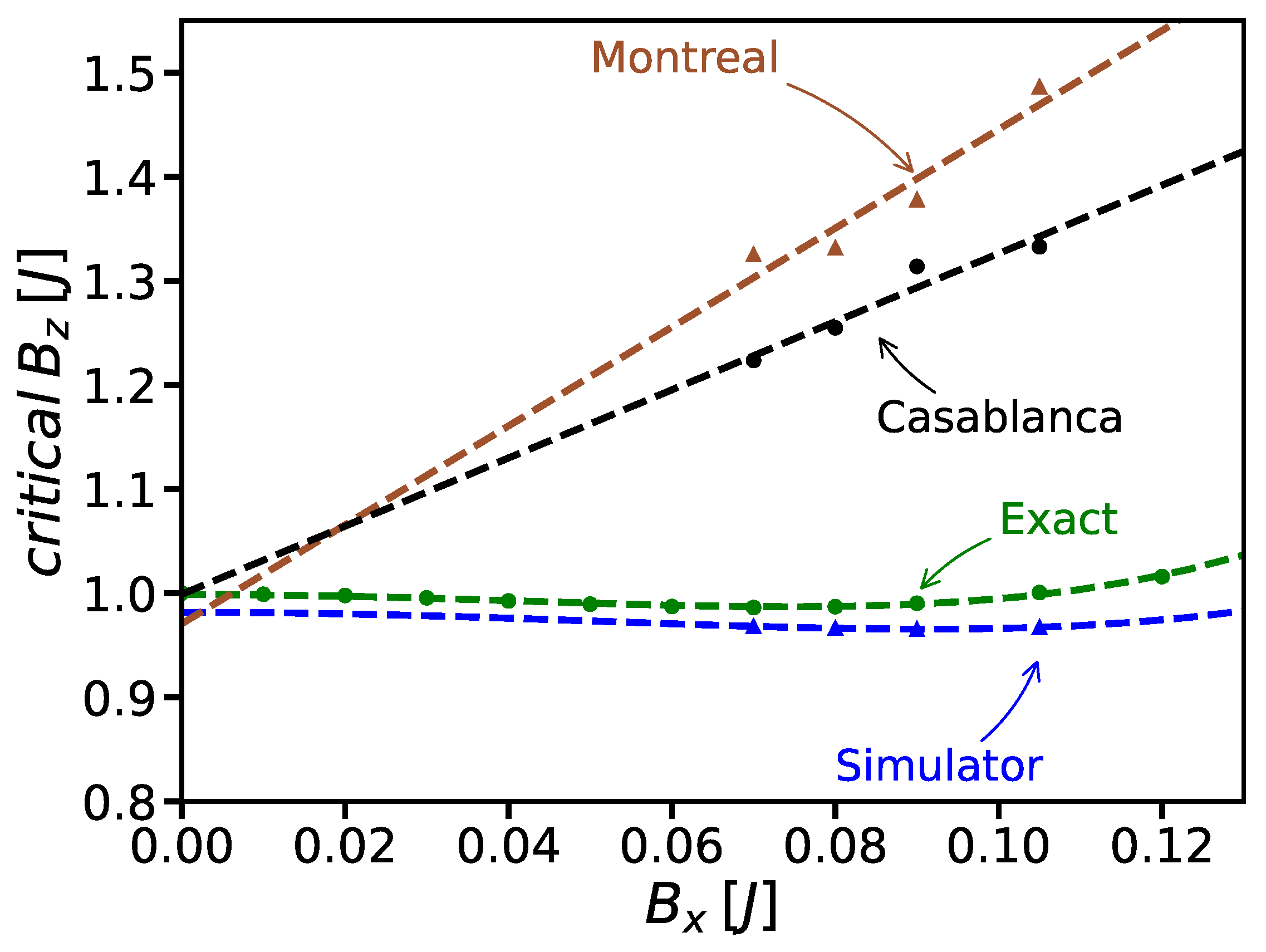
Extrapolation to find critical $B_z$ can be done by fitting polynomial curves to the data. The ${\sigma }^x$ operator only connects states with definite m eigenvalues that are shifted by one: $n=m\pm 1$, for $\langle n\left|{\sum }_i{\sigma }_i^x\right|m\rangle \ne 0$. Then, a simple argument using perturbation theory shows that the perturbed energy eigenvalues are functions of even powers of $B_x$ for small $B_x$ values. This means that when we try to extrapolate the exact results for the critical $B_z$ field, we should use a dependence on even powers of $B_x$ only. Hence, we include only quadratic and quartic terms in the fitting curve for the data generated on a classical computer via exact diagonalization.

For the data from a quantum computer, we instead fit with a linear regression, because the noise on the quantum computer changes the behavior from even powers of $B_x$ to a nearly linear dependence. When quantum computers become capable of doing longer time runs, with less noise and decoherence, then, we can fit a quadratic polynomial without the linear term for smaller $B_x$ values to estimate the critical point in a more systematic way.

3. Results

In order to demonstrate the technique, we first examine a two-site system. At large $B_z$, the ground state has all spins aligned in the up direction; the calculation starts with this state. The system is time evolved using the Trotter product formula using a local adiabatic ramp given in Equation (4). The integral produces $t\left(B_z\right)$ with uniform steps in $B_z$. We convert to $B_z\left(t\right)$ with uniform steps in t by inverting the map and employing an Akima spline, which preserves the shape (see Figure 3). We choose $\gamma$ and the number of time steps such that the time evolution spans the change in magnetization by one full unit (see Figure 4). We repeat the same procedure to find the time evolution for each $B_x$ value. The time evolution is implemented in the quantum simulation using two-qubit and single-qubit gates. We decompose each Trotter step into the XY part, the $B_x$ part, and the $B_z$ part:

$$\begin{array}{cc}\hfill {\mathbf{U}}_{12}\left(t+dt,t\right)& =exp\left[i[\frac{J}{4}\left({\sigma }_1^x{\sigma }_2^x+{\sigma }_1^y{\sigma }_2^y\right)+\frac{1}{2}{B}_x\left({\sigma }_1^x+{\sigma }_2^x\right)+\frac{1}{2}{B}_z\left(t\right)\left({\sigma }_1^z+{\sigma }_2^z\right)]dt\right]\hfill \end{array}$$

(7)

$$\begin{array}{cc}\hfill & \approx exp\left[i\frac{B_z\left(t\right)}{2}\left({\sigma }_1^z+{\sigma }_2^z\right)dt\right]exp\left[i\frac{B_x}{2}\left({\sigma }_1^x+{\sigma }_2^x\right)dt\right]exp\left[i\frac{J}{4}\left({\sigma }_1^x{\sigma }_2^x+{\sigma }_1^y{\sigma }_2^y\right)dt\right]\hfill \end{array}$$

(8)

The XY part is further decomposed to implement in the quantum simulation using two CNOTs [20], as shown in Figure 8. The $B_x$ part and $B_z$ part are implemented using single-qubit gates.

For the two-site case, we decrease $B_z$ from $B_z=1.0J$ to $B_z=0.0J$ to go through the first transition point (we have set $J=1$ in all our calculations). We use $B_x$ values given by $0.02J$, $0.03J$, $0.04J$, and $0.05J$ (see Figure 4). For the exact curve we use 1000 Trotter steps, but since we cannot achieve high fidelity in currently available quantum computers for such a large number of Trotter steps, we look for a similar trend in the crossing point so that a fewer number of Trotter time steps is sufficient (see Figure 6). For a two-site system the time evolution could be implemented with three CNOTs [20] to achieve high fidelity. But since these short-depth circuits are not available in general for a large system size, we consider the explicit implementation of a Trotter circuit to enable a comparison with larger system size. Later, we also show results from a three-CNOTs version of the circuit. With 20 Trotter steps the simulator data showed reasonable results. We use an Akima spline to fit the magnetization versus $B_z$ data to have a smooth curve, allowing us to determine the transition point. From the simulator data we find the crossing points where the magnetization is equal to 0.5. A quartic fit was performed to the crossing points from the simulator data and we obtained a critical value of $B_z=0.500J$. This result is reasonable, since performing a quartic fit to the first four data points in the exact curve yields an extrapolated value equal to $0.498J$.

We perform the quantum computer run on the ibmq_santiago. The data obtained from the quantum computer with measurement-error mitigation [19] is shown in Figure 4. As a secondary error mitigation technique, we scale the data so that the initial and final magnetization values of the quantum computer data match that of the quantum simulator. This stretches and shifts the data so that the end points have the correct values (see Figure 4). Such scaling is common to correct from decoherence and noise, and it improves the data analysis [21,22,23,24]. Here, scaling is based on the fact that for small $B_x$ values the magnetization approximately follows steps as a function of $B_z$. At our initial $B_z$, the magnetization corresponds to all spins aligned up; our final magnetization decreases by a single unit for each transition. When simulator values are difficult to obtain (e.g., for a large N) the final $B_z$ can be taken where the curve goes flat. The experiment is repeated for different $B_x$ values and the corresponding crossing points are plotted in the Figure 6. Since the data obtained was noisy we fitted a linear extrapolation curve to capture the trend in the quantum computer data. The extrapolated critical $B_z$ value is $0.504J$, which is close to the actual value of transition, which occurs at $0.5J$.

For the second case, we examine the transition from $m=-1$ to $m=0$. While, formally, this should be the same as the case for $m=1$ to $m=0$, because the $|1\rangle$ state of a quantum computer is the excited state, decoherence effects should be larger for this case. Here, the initial state has both spins down. The procedure is similar to what we explained above. A quartic fit to the simulator values obtained a critical value of $-0.50J$. A quartic fit to the first four data points of the exact crossings (for $\gamma$ = 1.5 and 1000 Trotter steps), obtained an extrapolated value of $-0.498J$. The data obtained from the IBM quantum computer is shown in Figure 4. The crossing points were found from the scaled data for each $B_x$ value. A linear fit to the quantum computer data gave the critical value to be $-0.54J$.

For the two-site model, we also performed the experiment in an ibmq_santiago machine after optimizing the circuits with a level-three optimization in the IBM Qiskit transpiler. This reduced the number of CNOT gates to three for each time step. This is because any two-qubit unitary operation can be represented using three-CNOT gates [20,25]. The read-out-corrected data are shown in Figure 4. The crossing points from these fixed-depth circuits are shown in Figure 6. These values are closer to the simulator values than the Trotter data, as expected. A quartic fit to these data obtained a critical $B_z$ value of $0.491J$ starting from all spins aligned up, and $-0.504J$ starting from all spins aligned down. This kind of an efficient fixed-depth decomposition is not known in general for more than two qubits. But for certain models, efficient fixed-depth circuit decompositions can be found [26]. These type of fixed-depth circuits can improve the performance of our method by reducing the number of gates in an adiabatic-time evolution as Trotter decomposition becomes increasingly costly with larger system sizes and more time evolution steps [27].

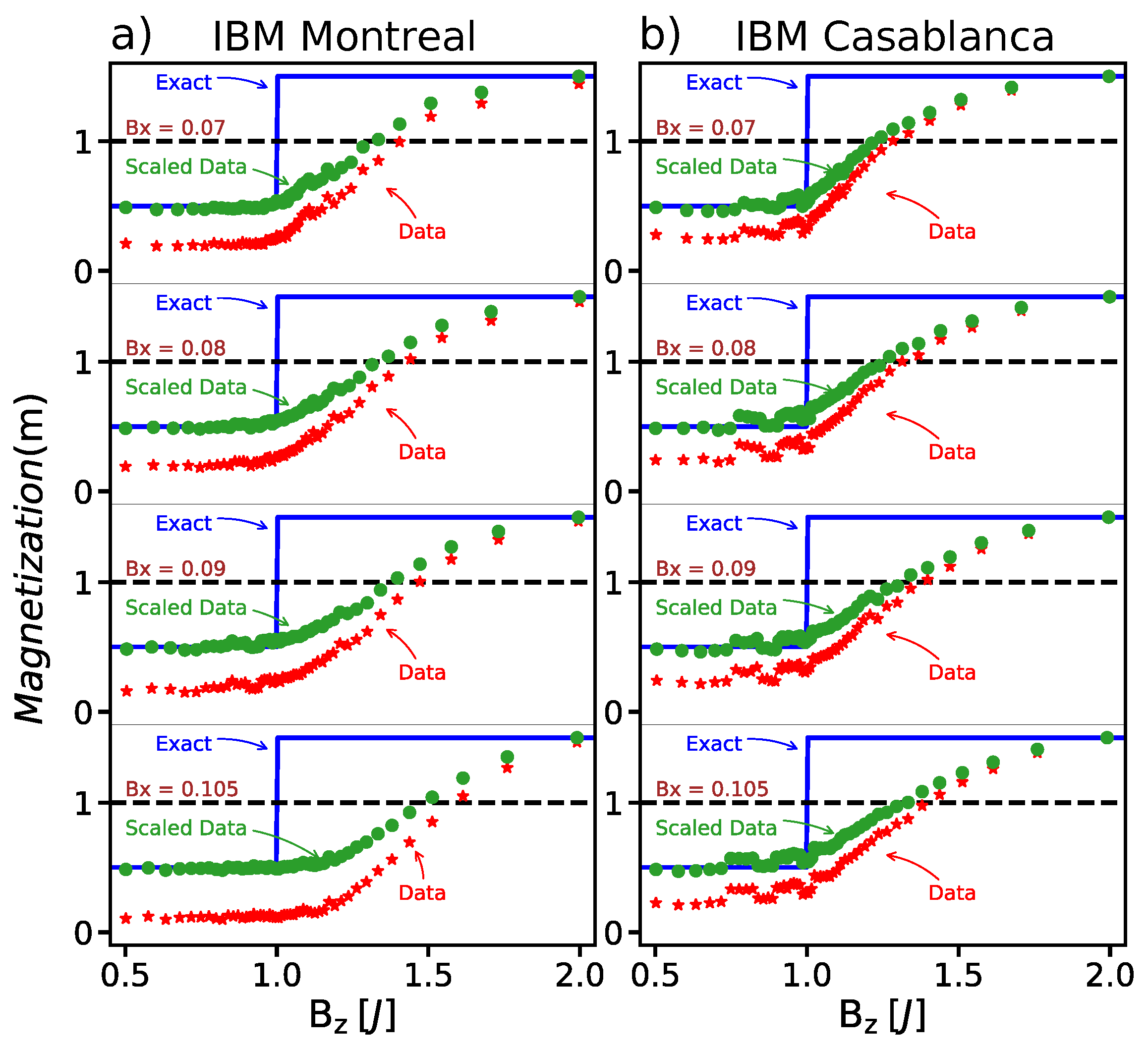
Now, we move on to the three-site periodic system. We start with all spins up. The time evolution circuit for the XY part is implemented pairwise using the XY part of the two-qubit circuit for each Trotter step. The data obtained from the quantum computer with measurement-error mitigation is shown in Figure 5, along with the scaled data which matches the end points from the simulator data. The extrapolations are shown in Figure 7. A quartic fit to the exact values gives the critical $B_z$ value to be $0.999J$. A quartic fit to the simulator values gives the critical $B_z$ to be $0.982J$. The linear fit to the crossings from the scaled data of the IBM quantum computer give the phase transition point to be $0.971J$ for ibmq_montreal and $0.999J$ for the ibmq_casablanca. The actual transition is at $1.0J$. These fitted values are reasonably close to the actual value.

4. Discussion

In this work, we propose a method for finding zero-temperature phase diagrams that are robust and can be carried out on quantum computers. The approach requires us to introduce a symmetry-breaking term into the Hamiltonian, determine approximate phase diagrams for the symmetry-broken system, and then extrapolate to the limit where the symmetry-breaking field vanishes. To verify that this approach works, we have worked out practical details for how to run these circuits on a quantum computer when the number of spins is two or three. The results from the quantum computers agree well with the exact results and are able to predict the phase boundaries within a few percent. This illustrates that the approach used here, based on adiabatic-state preparation, can work on NISQ machines and has the potential to be able to be applied to larger systems, even ones where we do not know the phase diagram a priori.

Note that the case we examined here, the XY model in a z-oriented magnetic field, is probably the most difficult problem to examine, because the number of level crossings increases with the system size. For most quantum phase transitions between different symmetry states, the number of phase boundaries should depend only weakly on the system size.

In order to show that this approach also applies to larger systems, we simulate the magnetization for a 10-site system in Figure 1 using a similar local adiabatic-time evolution for 1000 Trotter steps for $\gamma$ = 50. Extracting the phase transitions using our methodology works well for such a system, as can be seen by comparing the two lines in the figure.

As the system size increases, finer time-evolution steps are required to prepare the state due to the higher density of energy eigenstates. This would require the quantum hardware to have better gate fidelity and less measurement errors so that the overall error in magnetization remains low. Nevertheless, for larger and more complex systems, using quantum computers is a potential way to handle quantum-simulation-related problems, as classical computers cannot deal with very large Hilbert spaces in general [3,5]. Once better quantum hardware is available, our method could be applied to finding the critical points for larger quantum systems.