A Study on the Bertrand Offsets of Timelike Ruled Surfaces in Minkowski 3-Space

Abstract

This work extends some classical results of Bertrand curves to timelike ruled and developable surfaces using the E. Study map. This provides support to define two timelike ruled surfaces which are offset in the sense of Bertrand. It is proved that every timelike ruled surface has a Bertrand offset if and only if an equation should be satisfied among their dual invariants. In addition, some new results and theorems concerning the developability of the Bertrand offsets of timelike ruled surfaces are gained.

1. Introduction

In Euclidean 3-space, the trajectory of an oriented line embedded at a moving rigid body is generally a ruled surface. The geometry of ruled surfaces has been widely used in computer-aided manufacturing (CAM), computer-aided geometric design (CAGD), kinematics and geometric modeling [1,2,3]. Offset surfaces and ruled surfaces have been examined in Euclidean and non-Euclidean spaces: Ravani and Ku [4] generalized the theory of Bertrand curves for ruled and developable surfaces. It was shown that a ruled surface allows an infinity of Bertrand offsets, similarly as the planar curve allows an infinity of Bertrand mates. Based on the previous study, several properties of Bertrand offsets for trajectory ruled surfaces were obtained. In [5], Küçük and Gürsoy gave some characterizations of Bertrand offsets of trajectory ruled surfaces in terms of the relationships among the projection areas for the spherical images of Bertrand offsets and their integral invariants. In [6], Kasap and Kuruoglu obtained the relationships between the integral invariants of the pairs of a Bertrand ruled surface in Euclidean 3-space. In [7], the study of Bertrand offsets of ruled surfaces in Minkowski 3-space was initiated. The involute-evolute offsets of ruled surfaces were defined by Kasap et al. in [8]. Orbay et al. in [9] started the idea of Mannheim offsets in the case of a ruled surface. Onder and Ugurlu presented the relations between both invariants of Mannheim offsets of timelike ruled surfaces. In addition, the conditions for the offsets of this kind of surface to be developable were given in [10]. These offset surfaces are defined using the geodesic Frenet frame, which was given by [8]. According to involute-evolute offsets of the ruled surface in [10], the integral invariants of these offsets are calculated respecting the geodesic Frenet frame [11]. Important contributions to the Bertrand offsets of these ruled surfaces were investigated in [12,13,14,15,16].

In this paper, the principle of Bertrand curves is generalized and introduced for timelike ruled surfaces in Minkowski space. By using the E. Study map, two timelike ruled surfaces which are offset in the sense of Bertrand are defined. In particular, we investigate how to construct the Bertrand offset form, a timelike ruled surface with vanishing dual geodesic curvature. Meanwhile, a timelike developable surface can have a timelike developable Bertrand offset if a linear equation holds between the curvature and the torsion of its edge of regression.

Hopefully, the results in this paper will have some applications in the analysis of spatial motion and geometrical models.

2. Basic Concepts

We start with the basic concepts of dual numbers, dual Lorentzian vectors and the E. Study map (see [1,2,3,17,18,19]): An oriented (non-null) line in Minkowski 3-space will be defined using the point $\alpha \in L$ and the normalized direction vector $\mathbf{x}$ of L, that is, $\langle \mathbf{x},\mathbf{x}\rangle =\pm 1$. To acquire components of L, one forms the moment vector ${\mathbf{x}}^{*}=\alpha \times \mathbf{x}$ respecting the origin point at ${\mathbb{E}}_1^3$. In the case $\alpha$ that is replaced, one uses any point $\beta =\alpha +t\mathbf{x}$,$t\in \mathbb{R}$ at L, which shows that x${}^{*}$ is independent of $\alpha$ on L. In the case where two vectors $\mathbf{x}$ and ${\mathbf{x}}^{*}$ are not independent of each other, the following are satisfied:

$$\langle \mathbf{x},\mathbf{x}\rangle =\pm 1,\langle {\mathbf{x}}^{*},\mathbf{x}\rangle =0.$$

The six components $x_i,x_i^{*}(i=1,2,3)$ of $\mathbf{x}$ as well as ${\mathbf{x}}^{*}$ are named the normalized Plucker coordinates of the line L. Thus, the two vectors $\mathbf{x}$ and ${\mathbf{x}}^{*}$ locate the oriented line L.

The dual number $\widehat{x}$ is the number $x+\epsilon x^{*}$, where x and $x^{*}$ are real numbers and $\epsilon$ is the dual unit with the properties that $\epsilon \ne 0$ and ${\epsilon }^2=0$. Therefore, the set

$${\mathbb{D}}^3=\{\widehat{\mathbf{x}}:=\mathbf{x}+\epsilon {\mathbf{x}}^{*}=({\widehat{x}}_1,{\widehat{x}}_2,{\widehat{x}}_3)\},$$

with inner product

$$\langle \widehat{\mathbf{x}},\widehat{\mathbf{y}}\rangle =-{\widehat{x}}_1{\widehat{y}}_1+{\widehat{x}}_2{\widehat{y}}_2+{\widehat{x}}_3{\widehat{y}}_3,$$

defines the dual Lorentzian 3-space ${\mathbb{D}}_1^3$. Then,

$$\left.\begin{array}{c}{\widehat{\mathbf{f}}}_1\times {\widehat{\mathbf{f}}}_2={\widehat{\mathbf{f}}}_3,{\widehat{\mathbf{f}}}_1\times {\widehat{\mathbf{f}}}_3=-{\widehat{\mathbf{f}}}_2,{\widehat{\mathbf{f}}}_3\times {\widehat{\mathbf{f}}}_2={\widehat{\mathbf{f}}}_1,\hfill \\ -\langle {\widehat{\mathbf{f}}}_1,{\widehat{\mathbf{f}}}_1\rangle =\langle {\widehat{\mathbf{f}}}_2,{\widehat{\mathbf{f}}}_2\rangle =\langle {\widehat{\mathbf{f}}}_3,{\widehat{\mathbf{f}}}_3\rangle =1,\hfill \end{array}\right\}$$

where ${\widehat{\mathbf{f}}}_1$, ${\widehat{\mathbf{f}}}_2$ and ${\widehat{\mathbf{f}}}_3$ are the dual bases at the origin point $\mathbf{O}\left(0,0,0\right)$ of the dual Lorentzian 3-space ${\mathbb{D}}_1^3$. Consequently, the point $\widehat{x}={({\widehat{x}}_1,{\widehat{x}}_2,{\widehat{x}}_3)}^t$ has dual coordinates ${\widehat{x}}_i=(x_i+\epsilon x_i^{*})\in \mathbb{D}$. If $\mathbf{x}\ne \mathbf{0}$, the norm $∥\widehat{\mathbf{x}}∥$ of $\widehat{\mathbf{x}}=\mathbf{x}+\epsilon {\mathbf{x}}^{*}$ is

$$∥\widehat{\mathbf{x}}∥=\sqrt{\left|\langle \widehat{\mathbf{x}},\widehat{\mathbf{x}}\rangle \right|}=\sqrt{\left|\langle \mathbf{x},\mathbf{x}\rangle \right|},$$

and then the vector $\widehat{\mathbf{x}}$ is called the spacelike (respectively, timelike) dual unit vector in the case where $\langle \mathbf{x},\mathbf{x}\rangle =1$ (respectively, $\langle \mathbf{x},\mathbf{x}\rangle =-$1). It is clear that:

$$\langle \widehat{\mathbf{x}},\widehat{\mathbf{x}}\rangle =\pm 1⟺\langle \mathbf{x},\mathbf{x}\rangle =\pm 1,\langle \mathbf{x},{\mathbf{x}}^{*}\rangle =0.$$

The hyperbolicand Lorentzian (de Sitter space) dual unit spheres with center $\mathbf{O}$, respectively, are:

$${\mathbb{H}}_{+}^2=\left\{\widehat{\mathbf{x}}\in {\mathbb{D}}_1^3\mid -{\widehat{x}}_1^2+{\widehat{x}}_2^2+{\widehat{x}}_3^2=-1\right\},$$

and

$${\mathbb{S}}_1^2=\left\{\widehat{\mathbf{x}}\in {\mathbb{D}}_1^3\mid -{\widehat{x}}_1^2+{\widehat{x}}_2^2+{\widehat{x}}_3^2=1\right\}.$$

Then, the E. Study map is given as in [17]: A pair of conjugate hyperboloids shapes dual unit spheres. A set of null (lightlike) lines is represented by a common asymptotic cone, the ring-formed hyperboloid presents a set of spacelike lines, the oval-formed hyperboloid represents a set of timelike lines, and the pair of opposite vectors at the line is represented by the opposite points of every hyperboloid (Figure 1).

Definition 1.  

For any two non-null dual vectors $\widehat{\widehat{\mathbf{x}}}$ and $\widehat{\mathbf{y}}$ in ${\mathbb{D}}_1^3$, we have:

(i)

If $\widehat{\mathbf{x}}$ and $\widehat{\mathbf{y}}$ are two spacelike dual vectors, then

• If they span a spacelike dual plane, there is a unique dual number $\widehat{\phi }=\phi +\epsilon {\phi }^{*}$, $0\le \phi \le \pi$, and ${\phi }^{*}\in \mathbb{R}$ such that $<\widehat{\mathbf{x}},\widehat{\mathbf{y}}>=∥\widehat{\mathbf{x}}∥∥\widehat{\mathbf{y}}∥cos\widehat{\phi }$. This number is called the spacelike dual angle between $\widehat{\mathbf{x}}$ and $\widehat{\mathbf{y}}$.
• If they span a timelike dual plane, there is a unique dual number $\widehat{\phi }=\phi +\epsilon {\phi }^{*}\ge 0$ such that $<\widehat{\mathbf{x}},\widehat{\mathbf{y}}>=ϵ∥\widehat{\mathbf{x}}∥∥\widehat{\mathbf{y}}∥cosh\widehat{\phi }$, where $ϵ=+1$ or $ϵ=-1$ according to $sign\left({\widehat{x}}_2\right)=sign\left({\widehat{y}}_2\right)$ or $sign\left({\widehat{x}}_2\right)\ne sign\left({\widehat{y}}_2\right)$, respectively. This number is called the central dual angle between $\widehat{\mathbf{x}}$ and $\widehat{\mathbf{y}}$.

(ii)

If $\widehat{\mathbf{x}}$ and $\widehat{\mathbf{y}}$ are two timelike dual vectors, then there is a unique dual number $\widehat{\phi }=\phi +\epsilon {\phi }^{*}\ge 0$ such that $<\widehat{\mathbf{x}},\widehat{\mathbf{y}}>=ϵ∥\widehat{\mathbf{x}}∥∥\widehat{\mathbf{y}}∥cosh\widehat{\phi }$, where $ϵ=+1$ or $ϵ=-1$ according to whether $\widehat{\mathbf{x}}$ and $\widehat{\mathbf{y}}$ have different time orientations or the same time orientation, respectively. This dual number is called the Lorentzian timelike dual angle between $\widehat{\mathbf{x}}$ and $\widehat{\mathbf{y}}$.

(iii)

If $\widehat{\mathbf{x}}$ is spacelike dual and $\widehat{\mathbf{y}}$ is timelike dual, then there is a unique dual number $\widehat{\phi }=\phi +\epsilon {\phi }^{*}\ge$ 0 such that $<\widehat{\mathbf{x}},\widehat{\mathbf{y}}>=ϵ∥\widehat{\mathbf{x}}∥∥\widehat{\mathbf{y}}∥sinh\widehat{\phi }$, where $ϵ=+1$ or $ϵ=-1$ according to $sign\left({\widehat{x}}_2\right)=sign\left({\widehat{y}}_1\right)$ or $sign\left({\widehat{x}}_2\right)\ne sign\left({\widehat{y}}_1\right)$. This number is called the Lorentzian timelike dual angle between $\widehat{\mathbf{x}}$ and $\widehat{\mathbf{y}}$.

3. Bertrand Offsets of Timelike Ruled Surfaces

A timelike ruled surface is determined as a surface that is generated from the motion of an oriented timelike line along a curve in ${\mathbb{E}}_1^3$. Via the E. Study map, a timelike ruled surface is represented by the timelike dual unit vector of an arbitrary real parameter. Then, the dual spherical image, denoted by $\left(X\right)$, is a spacelike dual curve on the hyperbolic dual unit sphere ${\mathbb{H}}_{+}^2$, that is,

$$t\in \mathbb{R}\mapsto \widehat{\mathbf{x}}\left(t\right)\in {\mathbb{H}}_{+}^2.$$

where $\widehat{\mathbf{x}}\left(t\right)$ are specified using rulings of the surface and from here we do not distinguish between a ruled surface and its own representative dual curve. The vector

$$\widehat{\mathbf{t}}\left(t\right)=\mathbf{t}+\epsilon {\mathbf{t}}^{*}=\frac{d\widehat{\mathbf{x}}\left(t\right)}{dt}{∥\frac{d\widehat{\mathbf{x}}\left(t\right)}{dt}∥}^{-1}$$

is the spacelike dual unit tangent vector on $\widehat{\mathbf{x}}\left(t\right)$. Introducing the spacelike dual unit vector $\widehat{\mathbf{g}}\left(t\right)=\mathbf{g}\left(t\right)+\epsilon {\mathbf{g}}^{*}\left(t\right)=\widehat{\mathbf{x}}\times \widehat{\mathbf{t}}$, we have the moving frame {$\widehat{\mathbf{x}}\left(t\right),$ $\widehat{\mathbf{t}}\left(t\right),$ $\widehat{\mathbf{g}}\left(t\right)\}$ on $\widehat{\mathbf{x}}\left(t\right)$ called the Blaschke frame. Then,

$$\left.\begin{array}{c}\hfill -\langle \widehat{\mathbf{x}},\widehat{\mathbf{x}}\rangle =\langle \widehat{\mathbf{t}},\widehat{\mathbf{t}}\rangle =\langle \widehat{\mathbf{g}},\widehat{\mathbf{g}}\rangle =1,\\ \hfill \widehat{\mathbf{g}}=\widehat{\mathbf{x}}\times \widehat{\mathbf{t}},\widehat{\mathbf{x}}=\widehat{\mathbf{t}}\times \widehat{\mathbf{g}},-\widehat{\mathbf{t}}=\widehat{\mathbf{x}}\times \widehat{\mathbf{g}}.\end{array}\right\}$$

The Blaschke formula is [17]:

$$\frac{d}{dt}\left(\begin{array}{c}\widehat{\mathbf{x}}\hfill \\ \widehat{\mathbf{t}}\hfill \\ \widehat{\mathbf{g}}\hfill \end{array}\right)=\left(\begin{array}{ccc}0\hfill & \widehat{p}\hfill & 0\hfill \\ \widehat{p}\hfill & 0\hfill & \widehat{q}\hfill \\ 0\hfill & -\widehat{q}\hfill & 0\hfill \end{array}\right)\left(\begin{array}{c}\widehat{\mathbf{x}}\hfill \\ \widehat{\mathbf{t}}\hfill \\ \widehat{\mathbf{g}}\hfill \end{array}\right),$$

(1)

where

$$\widehat{p}\left(t\right)=p\left(t\right)+\epsilon p^{*}\left(t\right)=∥\frac{d\widehat{\mathbf{x}}\left(t\right)}{dt}∥,\widehat{q}=q+\epsilon q^{*}=det(\widehat{\mathbf{x}},\frac{d\widehat{\mathbf{x}}\left(t\right)}{dt},\frac{d^2\widehat{\mathbf{x}}\left(t\right)}{d{t}^2}),$$

(2)

are named the Blaschke invariants of the spacelike dual curve $\widehat{\mathbf{x}}\left(t\right)$. The dual unit vectors $\widehat{\mathbf{x}}$, $\widehat{\mathbf{t}}$ and $\widehat{\mathbf{g}}$ correspond to three concurrent mutually orthogonal oriented lines in ${\mathbb{E}}_1^3$ and they intersect at the point $\mathbf{c}$ on $\widehat{\mathbf{x}}$ named the striction (or central) point. The trajectory of the central point is named the striction curve on $\left(X\right)$. The dual arc-length $\widehat{s}$ of $\widehat{\mathbf{x}}\left(t\right)$ is defined as

$$d\widehat{s}=ds+\epsilon d{s}^{*}=∥\frac{d\widehat{\mathbf{x}}\left(t\right)}{dt}∥dt=\widehat{p}\left(t\right)dt.$$

(3)

The distribution parameter of the ruled surface is

$$\mu \left(t\right):=\frac{d{s}^{*}}{ds}=\frac{p^{*}\left(t\right)}{p\left(t\right)}.$$

(4)

From Equations (1) and (3), we also obtain [17]:

$$\left(\begin{array}{c}{\widehat{\mathbf{x}}}^{{}^{\prime }}\hfill \\ {\widehat{\mathbf{t}}}^{{}^{\prime }}\hfill \\ {\widehat{\mathbf{g}}}^{{}^{\prime }}\hfill \end{array}\right)=\left(\begin{array}{ccc}0\hfill & 1\hfill & 0\hfill \\ 1\hfill & 0\hfill & \widehat{\gamma }\hfill \\ 0\hfill & -\widehat{\gamma }\hfill & 0\hfill \end{array}\right)\left(\begin{array}{c}\widehat{\mathbf{x}}\hfill \\ \widehat{\mathbf{t}}\hfill \\ \widehat{\mathbf{g}}\hfill \end{array}\right)=\widehat{\omega }\times \left(\begin{array}{c}\widehat{\mathbf{x}}\hfill \\ \widehat{\mathbf{t}}\hfill \\ \widehat{\mathbf{g}}\hfill \end{array}\right);{(}^{\prime }=\frac{d}{d\widehat{s}}),$$

(5)

where $\widehat{\omega }=\omega +\epsilon {\omega }^{*}=\widehat{\chi }\widehat{\mathbf{x}}-\widehat{\mathbf{g}}$ is the Darboux vector and $\widehat{\gamma }\left(\widehat{s}\right):=\gamma +\epsilon {\gamma }^{*}$ is the dual geodesic curvature of $\widehat{\mathbf{x}}\left(\widehat{s}\right)$ on ${\mathbb{H}}_{+}^2$. The tangent vector to the striction curve $\mathbf{c}\left(s\right)$ is given by

$$\frac{d\mathbf{c}}{ds}=-\Gamma \left(s\right)\mathbf{x}+\mu \left(s\right)\mathbf{g},$$

(6)

which is a spacelike (respectively, a timelike) curve if $\left|\mu \right|>\left|\Gamma \right|$ (respectively, $\left|\mu \right|<\left|\Gamma \right|$) [17]. The functions $\gamma \left(s\right)$, $\Gamma \left(s\right)$ and $\mu \left(s\right)$ are the curvature (construction) functions of the ruled surface. These functions are described as follows:$\gamma$ is the geodesic curvature of the spacelike spherical image curve $\mathbf{x}=\mathbf{x}\left(s\right)$, $\Gamma$ describes the angle among the ruling of $\left(X\right)$ and the tangent to the striction curve, and $\mu$ is its distribution parameter at the ruling. These functions define a method for establishing timelike ruled surfaces by the equation

$$\left(X\right):\mathbf{y}(s,v)=\stackrel{s}{\underset{0}{\int }}\left(-\Gamma \left(s\right)\mathbf{x}\left(s\right)+\mu \left(s\right)\mathbf{g}\left(s\right)\right)ds+v\mathbf{x}\left(s\right).$$

(7)

The unit normal vector field $\mathbf{e}$ is

$$\mathbf{e}(s,v)=\frac{\frac{\partial \mathbf{y}(s,v)}{\partial s}\times \frac{\partial \mathbf{y}(s,v)}{\partial v}}{∥\frac{\partial \mathbf{y}(s,v)}{\partial s}\times \frac{\partial \mathbf{y}(s,v)}{\partial v}∥}=\pm \frac{\mu \mathbf{t}+v\mathbf{g}}{\sqrt{{\mu }^2+v^2}},$$

(8)

which is the spacelike central normal at the striction point ($v=0$). Let $\varphi$ be the angle between $\mathbf{e}$ and $\mathbf{t}$. Then,

$$\mathbf{e}(s,v)=cos\varphi \mathbf{t}+sin\varphi \mathbf{g}.$$

It is clear that:

$$tan\varphi =\frac{v}{\mu }.$$

This result is a Minkowski version of the well-known Chasles Theorem [1,2,3]. Hence, we have the following:

Corollary 1.

The tangent plane of the nondevelopable timelike ruled surface (X) turns clearly through π along a ruling.

Under the assumption that $\left|\widehat{\gamma }\right|<1$, we also specify the spacelike Disteli-axis:

$$\widehat{\mathbf{b}}\left(\widehat{s}\right):=\mathbf{b}+\epsilon {\mathbf{b}}^{*}=\frac{\widehat{\omega }}{∥\widehat{\omega }∥}=\frac{\widehat{\chi }\widehat{\mathbf{x}}+\widehat{\mathbf{g}}}{\sqrt{1-{\widehat{\gamma }}^2}}=sinh\widehat{\psi }\widehat{\mathbf{x}}-cosh\widehat{\psi }\widehat{\mathbf{g}},$$

(9)

where $\widehat{\psi }=\psi +\epsilon {\psi }^{*}$ is the dual radius of curvature between $\widehat{\mathbf{b}}$ and $\widehat{\mathbf{x}}$. The dual geodesic curvature $\widehat{\gamma }\left(\widehat{s}\right)$ in terms of $\Gamma$, $\mu$ and $\gamma$ is [17]:

$$\widehat{\gamma }\left(\widehat{s}\right)=\gamma +\epsilon \left(\Gamma -\gamma \mu \right)=tanh\widehat{\psi }.$$

(10)

Moreover, we also have:

$$\left.\begin{array}{c}\widehat{\gamma }\left(\widehat{s}\right)=\gamma +\epsilon \left(\Gamma -\gamma \mu \right)=tanh\psi +\epsilon {\psi }^{*}(1-{tanh}^2\psi ),\hfill \\ \widehat{\kappa }\left(\widehat{s}\right):=\kappa +\epsilon {\kappa }^{*}=\sqrt{1-{\widehat{\gamma }}^2}=\frac{1}{cosh\widehat{\psi }},\hfill \\ \widehat{\tau }\left(\widehat{s}\right):=\tau +\epsilon {\tau }^{*}=\pm {\widehat{\psi }}^{{}^{\prime }}=\pm \frac{{\widehat{\gamma }}^{{}^{\prime }}}{1-{\widehat{\gamma }}^2},\hfill \end{array}\right\}$$

(11)

where $\widehat{\kappa }\left(\widehat{s}\right)$ is the dual curvature and $\widehat{\tau }\left(\widehat{s}\right)$ is the dual torsion of the spacelike dual curve $\widehat{\mathbf{x}}\left(\widehat{s}\right)\in {\mathbb{H}}_{+}^2$.

Proposition 1.

If the dual geodesic curvature function $\widehat{\gamma }\left(\widehat{s}\right)$ is constant, $\widehat{\mathbf{x}}\left(\widehat{s}\right)$ is a dual circle on ${\mathbb{H}}_{+}^2$.

Proof. 

From Equation (11) we can find that having $\widehat{\gamma }\left(\widehat{s}\right)$ constant yields that $\widehat{\tau }\left(\widehat{s}\right)=0$, and if $\widehat{\kappa }\left(\widehat{s}\right)$ is constant, that leads to $\widehat{\mathbf{x}}\left(\widehat{s}\right)$ being a spacelike dual circle on ${\mathbb{H}}_{+}^2$. □

Definition 2.

A nondevelopable timelike ruled surface $\left(X\right)$ is defined as a constant Disteli-axis timelike ruled surface if its dual geodesic curvature $\widehat{\gamma }\left(\widehat{s}\right)$ is constant.

According to the E. Study map, the constant Disteli-axis timelike ruled surface (X) is formed by a one-parameter helical motion with constant pitch h about the spacelike Disteli-axis $\widehat{\mathbf{b}}$, by the oriented timelike line $\widehat{\mathbf{x}}$ situated at a Lorentzian constant distance ${\psi }^{*}$ and a Lorentzian constant angle $\psi$ relative to the timelike Disteli-axis $\widehat{\mathbf{b}}$. The constant Disteli-axis is essential to the curvature theory of ruled surfaces. Therefore, we will investigate some of its properties later. As a special case, if $\widehat{\gamma }\left(\widehat{s}\right)=0$, then $\widehat{\mathbf{x}}\left(\widehat{s}\right)$ is a spacelike great dual circle on ${\mathbb{H}}_{+}^2$, that is,

$$\widehat{\mathbf{c}}=\{\widehat{\mathbf{x}}\in {\mathbb{H}}_{+}^2\mid \langle \widehat{\mathbf{x}},\widehat{\mathbf{b}}\rangle =0,\mathrm{with}\parallel \widehat{\mathbf{b}}\parallel =1\}.$$

In this case, all the rulings of (X) intersect orthogonally with the spacelike Disteli-axis $\widehat{\mathbf{b}}$, that is, $\psi ={\psi }^{*}=0$. Thus, we have $\widehat{\gamma }\left(\widehat{s}\right)=0\iff \left(X\right)$ is a timelike helicoidal surface.

Now, we give a kinematic interpretation of $\widehat{\gamma }\left(\widehat{s}\right)$ as follows: If $\mathbf{x}\left(\widehat{s}\right)=\widehat{\mathbf{x}}(\widehat{s}+2\pi )$, then $\mathbf{x}\left(\widehat{s}\right)$ is a closed curve on ${\mathbb{H}}_{+}^2$. According to the E. Study map, this curve corresponds to an (X)-closed timelike ruled surface in ${\mathbb{E}}_1^3$. We define a spacelike dual unit vector $\widehat{\mathbf{u}}$ rigidly linked with the Blaschke frame {$\widehat{\mathbf{x}}\left(\widehat{s}\right),$ $\widehat{\mathbf{t}}\left(\widehat{s}\right),$ $\widehat{\mathbf{g}}\left(\widehat{s}\right)\}$ such that the spacelike oriented line corresponding to $\widehat{\mathbf{u}}$ generates a timelike developable ruled surface (timelike torse) among the orthogonal trajectory of the (X)-closed timelike ruled surface. Then, the spacelike dual unit vector $\widehat{\mathbf{u}}$ can be represented as

$$\widehat{\mathbf{u}}\left(\widehat{s}\right)=sin\widehat{\beta }\left(\widehat{s}\right)\widehat{\mathbf{t}}\left(\widehat{s}\right)+cos\widehat{\beta }\left(\widehat{s}\right)\widehat{\mathbf{g}}\left(\widehat{s}\right),\mathrm{with}\widehat{\beta }=\beta +\epsilon {\beta }^{*},$$

from which we obtain

$${\widehat{\mathbf{u}}}^{{}^{\prime }}\left(\widehat{s}\right){=(\widehat{\beta }}^{{}^{\prime }}-\widehat{\gamma }){\widehat{\mathbf{u}}}^{\perp }+sinh\widehat{\beta }\widehat{\mathbf{x}}\left(\widehat{s}\right).$$

Then, we call the total change of $\widehat{\beta }\left(\widehat{s}\right)$ the dual angle of pitch of the (X)-closed timelike ruled surface, that is,

$$\oint d\widehat{\beta }=\oint \widehat{\gamma }d\widehat{s}=-\oint \langle \widehat{\mathbf{t}},{\widehat{\mathbf{g}}}^{{}^{\prime }}\rangle d\widehat{s}.$$

(12)

It is separated into real and dual parts as:

$$\oint d\beta =\oint \gamma \left(s\right)ds,\mathrm{and}\oint d{\beta }^{*}=\oint \Gamma \left(s\right)ds.$$

(13)

Hence, we arrive therefore at the conclusions that:

• The angle pitch of an (X)-closed timelike ruled surface is

  $${\lambda }_x\left(s\right)=\oint \gamma \left(s\right)ds=-\oint \langle \mathbf{t},\frac{d\mathbf{g}}{ds}\rangle ds,$$

  (14)
• The pitch of an (X)-closed timelike ruled surface is

  $$L_x\left(s\right)=\oint \Gamma \left(s\right)ds=-\oint \langle \mathbf{x},\frac{d\mathbf{c}}{ds}\rangle ds.$$

  (15)

The pitch $L_x$ and the angle of pitch ${\lambda }_x$ are integral invariants of an ($\overline{X}$)-closed timelike ruled surface. Then,

$${\Lambda }_x\left(\widehat{s}\right)={\lambda }_x+\epsilon L_x=\oint d\widehat{\beta }=-\oint \langle \widehat{\mathbf{t}},{\widehat{\mathbf{g}}}^{{}^{\prime }}\rangle d\widehat{s},$$

(16)

is the Minkowski version of the dual angle of pitch defined in [5,12,20,21].

Corollary 2.

Any timelike ruled surface (X) is a timelike helicoidal surface iff its dual angle of pitch $\widehat{\Lambda }\left(\widehat{s}\right)$ is identically zero.

Notice that in Equation (7):

(a) When $\mu \left(s\right)=0$ ($\frac{d\mathbf{c}}{ds}\Vert \mathbf{x}$), the Blaschke frame $\left\{\mathbf{x}\right(s),$ $\mathbf{t}\left(s\right)$, $\mathbf{g}\left(s\right)\}$ is the usual Serret–Frenet frame, that is, ${\zeta }_1=-\mathbf{x}\left(s\right)$, ${\zeta }_2=-\mathbf{t}\left(s\right)$ and ${\zeta }_3=\mathbf{g}\left(s\right)$. Then, $\left(X\right)$ is a timelike tangential developable ruled surface (timelike tangential surface for short). Let u be the arc length parameter of $\mathbf{c}\left(s\right)$ and $\{{\zeta }_1\left(u\right),$${\zeta }_2\left(u\right)$, ${\zeta }_3\left(u\right)\}$ be the usual moving Serret–Frenet frame of $\mathbf{c}\left(s\right)$. Then,

$$\frac{d}{du}\left(\begin{array}{c}{\zeta }_1\left(u\right)\hfill \\ {\zeta }_2\left(u\right)\hfill \\ {\zeta }_3\left(u\right)\hfill \end{array}\right)=\left(\begin{array}{ccc}0\hfill & \kappa \left(u\right)\hfill & 0\hfill \\ \kappa \left(u\right)\hfill & 0\hfill & -\tau \left(u\right)\hfill \\ 0\hfill & \tau \left(u\right)\hfill & 0\hfill \end{array}\right)\left(\begin{array}{c}{\zeta }_1\left(u\right)\hfill \\ {\zeta }_2\left(u\right)\hfill \\ {\zeta }_3\left(u\right)\hfill \end{array}\right),$$

where $\kappa \left(u\right)$ and $\tau \left(u\right)$ are the natural curvature and torsion of the striction curve $\mathbf{c}\left(u\right)$, in the same order:

$$\kappa \left(u\right)=\frac{1}{\Gamma \left(u\right)},\tau \left(u\right)=\frac{\gamma \left(u\right)}{\Gamma \left(u\right)},\mathrm{with}\Gamma \left(u\right)\ne 0.$$

Therefore, the curvature function $\Gamma \left(u\right)$ is the radius of curvature of the timelike striction curve $\mathbf{c}\left(u\right)$. We arrive therefore at the conclusion that the timelike striction curve $\mathbf{c}\left(u\right)$ is the regression edge of $\left(X\right)$. Based on [22], the result is summarized as the following:

Theorem 1.

Any timelike ruled surface (X) with the curvature function

$$\Gamma \left(u\right)=acos\stackrel{u}{\underset{0}{\int }}\tau \left(u\right)du+bsin\stackrel{u}{\underset{0}{\int }}\tau \left(u\right)du;\tau \left(u\right)\ne 0,$$

with real constants $(a,b)\ne (0,0)$ is a timelike tangential surface of a timelike curve lying on a Lorentzian sphere with radius $\sqrt{a^2+b^2}$.

(b) If $\Gamma \left(s\right)=0$, then the striction curve is tangent to $\mathbf{g}$, it is normal to the ruling through $\mathbf{c}\left(s\right)$, ${\zeta }_1=\mathbf{g}\left(s\right)$, ${\zeta }_2=-\mathbf{t}\left(s\right)$ and ${\zeta }_3=\mathbf{x}\left(s\right)$. In this case, (X) a timelike binormal ruled surface. Similarly, we find

$$\frac{d}{du}\left(\begin{array}{c}{\zeta }_1\left(u\right)\hfill \\ {\zeta }_2\left(u\right)\hfill \\ {\zeta }_3\left(u\right)\hfill \end{array}\right)=\left(\begin{array}{ccc}0\hfill & \kappa \left(u\right)\hfill & 0\hfill \\ -\kappa \left(u\right)\hfill & 0\hfill & -\tau \left(u\right)\hfill \\ 0\hfill & -\tau \left(u\right)\hfill & 0\hfill \end{array}\right)\left(\begin{array}{c}{\zeta }_1\left(u\right)\hfill \\ {\zeta }_2\left(u\right)\hfill \\ {\zeta }_3\left(u\right)\hfill \end{array}\right),$$

where $\kappa \left(u\right)$ and $\tau \left(u\right)$ are the natural curvature and torsion of the striction curve $\mathbf{c}\left(u\right)$, respectively:

$$\kappa \left(u\right)=\frac{\gamma \left(u\right)}{\mu \left(u\right)},\tau \left(u\right)=\frac{1}{\mu \left(u\right)},\mathrm{with}\mu \left(u\right)\ne 0.$$

Therefore, the curvature function $\mu \left(u\right)$ is the radius of torsion of the spacelike striction curve $\mathbf{c}\left(s\right)$. The result is summarized as the following:

Theorem 2.

Any timelike ruled surface (X) with the curvature function

$$\frac{\mu \left(u\right)}{\gamma \left(u\right)}=cosh\stackrel{u}{\underset{0}{\int }}\tau \left(u\right)du-bsinh\stackrel{u}{\underset{0}{\int }}\tau \left(u\right)du;\tau \left(u\right)\ne 0,$$

with real constants $(a,b)\ne (0,0)$ is a timelike binormal surface of a spacelike curve lying on a Lorentzian sphere with radius $\sqrt{a^2-b^2}>0$.

Definition 3.

Let $\left(X\right)$ and ($\overline{X}$) be two timelike ruled surfaces in ${\mathbb{E}}_1^3$. ($\overline{X}$) is named the Bertrand offset of $\left(X\right)$ if there is a one-to-one correspondence between their rulings, that is, both surfaces have a common spacelike central normal at the striction points of their corresponding rulings.

Suppose a timelike ruled surface ($\overline{X}$) is represented by a timelike dual unit vector

$$\widehat{\overline{\mathbf{x}}}\left(\widehat{s}\right):=\overline{\mathbf{x}}+\epsilon {\overline{\mathbf{x}}}^{*}={\widehat{x}}_1\widehat{\mathbf{x}}+{\widehat{x}}_2\widehat{\mathbf{t}}+{\widehat{x}}_3\widehat{\mathbf{g}},$$

(17)

where ${\widehat{x}}_i={\widehat{x}}_i\left(\widehat{s}\right),(i=1,2,3)$, are its dual coordinate functions. Therefore,

$$-{\widehat{x}}_1^2+{\widehat{x}}_2^2+{\widehat{x}}_3^2=-1.$$

(18)

Differentiating Equations (17) and (18) with the aid of Equation (5), we find:

$$\left.\begin{array}{c}{\widehat{\overline{\mathbf{x}}}}^{{}^{{}^{\prime }}}=({\widehat{x}}_1^{{}^{{}^{\prime }}}+{\widehat{x}}_2)\widehat{\mathbf{x}}+({\widehat{x}}_2^{{}^{{}^{\prime }}}+{\widehat{x}}_1-\widehat{\gamma }{\widehat{x}}_3)\widehat{\mathbf{t}}+({\widehat{x}}_3^{{}^{{}^{\prime }}}+\widehat{\gamma }{\widehat{x}}_2)\widehat{\mathbf{g}},\hfill \\ -{\widehat{x}}_1{\widehat{x}}_1^{{}^{{}^{\prime }}}+{\widehat{x}}_2{\widehat{x}}_2^{{}^{{}^{\prime }}}+{\widehat{x}}_3{\widehat{x}}_3^{{}^{{}^{\prime }}}=0.\hfill \end{array}\right\}$$

(19)

If we suppose that the dual curves $\widehat{\overline{\mathbf{x}}}=\widehat{\overline{\mathbf{x}}}\left(\widehat{s}\right)$ and $\widehat{x}$=$\widehat{x}$$\left(\widehat{s}\right)$ are Bertrand offsets, that is, $\widehat{\mathbf{t}}=\widehat{\overline{\mathbf{t}}}$, then we have:

$${\widehat{x}}_1^{{}^{{}^{\prime }}}+{\widehat{x}}_2=0,{\widehat{x}}_2^{{}^{{}^{\prime }}}+{\widehat{x}}_1-\widehat{\gamma }{\widehat{x}}_3=-\langle {\overline{\widehat{\mathbf{x}}}}^{{}^{{}^{\prime }}},\widehat{\mathbf{t}}\rangle ,{\widehat{x}}_3^{{}^{{}^{\prime }}}+\widehat{\gamma }{\widehat{x}}_2=0.$$

(20)

Substituting Equation (20) in the second equation of (19) and simplifying it leads to

$${\widehat{x}}_2=0.$$

(21)

From (19) and (21), we obtain

$${\widehat{x}}_1^{{}^{{}^{\prime }}}=0,{\widehat{x}}_1+\widehat{\gamma }{\widehat{x}}_3=\langle {\overline{\widehat{\mathbf{x}}}}^{{}^{{}^{\prime }}},\widehat{\mathbf{t}}\rangle ,{\widehat{x}}_3^{{}^{{}^{\prime }}}=0\Rightarrow {\widehat{x}}_1={\widehat{c}}_{1,}{\widehat{x}}_3=\widehat{c_3}\in \mathbb{D},$$

(22)

where ${\widehat{c}}_1$ and ${\widehat{c}}_3$ are the dual constants of integrations. Hence, we define a constant hyperbolic dual angle $\widehat{\vartheta }=\vartheta +\epsilon {\vartheta }^{*}$ such that ${\widehat{c}}_1=cosh\widehat{\vartheta }$ and ${\widehat{c}}_3=sinh\widehat{\vartheta }$. Therefore, the following theorem is proved:

Theorem 3.

The offset hyperbolic dual angle formed by the generating timelike lines of a nondevelopable timelike ruled surface and its timelike Bertrand offset at corresponding central points remains constant.

It is obvious from the above developments that the timelike ruled surface, generally, has a double infinity of timelike Bertrand offsets. Every timelike Bertrand offset may be generated using a hyperbolic constant linear offset ${\vartheta }^{*}\in \mathbb{R}$ and a hyperbolic constant angular offset $\vartheta \in \mathbb{R}.$ Any two timelike surfaces of this family of timelike ruled surfaces are reciprocal of one another; in the case where ($\overline{X}$) is the timelike Bertrand offset of (X), then (X) is also a timelike Bertrand offset of ($\overline{X}$). Thus, Equation (17) becomes:

$$\widehat{\overline{\mathbf{x}}}\left(\widehat{s}\right)=cosh\widehat{\vartheta }\widehat{\mathbf{x}}\left(\widehat{s}\right)+sinh\widehat{\vartheta }\widehat{\mathbf{g}}\left(\widehat{s}\right).$$

(23)

In view of Definition 3, that for a ruled surface and its Bertrand offset the central normals coincide, it follows from the above theorem that the central tangents of the two timelike ruled surfaces also have the same constant dual angle at the corresponding points on the two striction curves. Then,

$$\widehat{\overline{\mathbf{g}}}=sinh\widehat{\vartheta }\widehat{\mathbf{x}}\left(\widehat{s}\right)+cosh\widehat{\vartheta }\widehat{\mathbf{g}}\left(\widehat{s}\right).$$

Hence, the Blaschke frame of ($\overline{X}$) can be given as follows:

$$\left(\begin{array}{c}\widehat{\overline{\mathbf{x}}}\left(\widehat{s}\right)\hfill \\ \widehat{\overline{\mathbf{t}}}\left(\widehat{s}\right)\hfill \\ \widehat{\overline{\mathbf{g}}}\left(\widehat{s}\right)\hfill \end{array}\right)=\left(\begin{array}{ccc}cosh\widehat{\vartheta }\hfill & 0\hfill & sinh\widehat{\vartheta }\hfill \\ 0\hfill & 1\hfill & 0\hfill \\ sinh\widehat{\vartheta }\hfill & 0\hfill & cosh\widehat{\vartheta }\hfill \end{array}\right)\left(\begin{array}{c}\widehat{\mathbf{x}}\left(\widehat{s}\right)\hfill \\ \widehat{\mathbf{t}}\left(\widehat{s}\right)\hfill \\ \widehat{\mathbf{g}}\left(\widehat{s}\right)\hfill \end{array}\right).$$

(24)

Notice that the previous equation is exactly the same as its similar equation for Bertrand curves [4]. If $\vartheta =0$ (respectively, ${\vartheta }^{*}=0$), the timelike Bertrand offsets are called oriented (respectively, coincident) offsets. Using Equations (16) and (24), we obtain that the dual angle of pitch of an ($\overline{X}$)-closed timelike ruled surface is given by:

$${\Lambda }_{\overline{x}}={\Lambda }_{x}cosh\widehat{\vartheta }+{\Lambda }_{g}sinh\widehat{\vartheta }.$$

(25)

This is a new characterization of Bertrand offsets of closed timelike ruled surfaces among their dual invariants. Then, the following theorem can be given.

Theorem 4.

The nondevelopable timelike ruled surfaces ($\overline{X}$) and (X) form a Bertrand offset iff Equation (25) is satisfied.

Corollary 3.

The Bertrand offset $\left(\overline{X}\right)$ of a timelike helicoidal surface, generally, does not have to be a timelike helicoidal surface and can be a regular timelike ruled surface.

From the real and dual parts of Equation (25), the following are obtained:

$$\left.\begin{array}{c}\hfill {\lambda }_{\overline{x}}={\lambda }_{x}cosh\vartheta +{\lambda }_{g}sinh\vartheta ,\\ \\ \hfill L_{\overline{x}}=(L_x-{\vartheta }^{*}{\lambda }_g)cosh\vartheta +(L_g-{\vartheta }^{*}{\lambda }_x)sinh\vartheta ,\end{array}\right\}$$

(26)

This is a Lorentzian version of Holditch’s Theorem [5,12,20,22].

Let $\widehat{\overline{s}}$ be the dual arc length of $\widehat{\overline{\mathbf{x}}}\left(\widehat{s}\right)\in {\mathbb{H}}_{+}^2$. Then,

$$\frac{d}{d\widehat{\overline{s}}}\left(\begin{array}{c}\widehat{\overline{\mathbf{x}}}\left(\widehat{s}\right)\hfill \\ \widehat{\overline{\mathbf{t}}}\left(\widehat{s}\right)\hfill \\ \widehat{\overline{\mathbf{g}}}\left(\widehat{s}\right)\hfill \end{array}\right)=\left(\begin{array}{ccc}0\hfill & 1\hfill & 0\hfill \\ 1\hfill & 0\hfill & \widehat{\overline{\gamma }}\hfill \\ 0\hfill & -\widehat{\overline{\gamma }}\hfill & 0\hfill \end{array}\right)\left(\begin{array}{c}\widehat{\overline{\mathbf{x}}}\left(\widehat{s}\right)\hfill \\ \widehat{\overline{\mathbf{t}}}\left(\widehat{s}\right)\hfill \\ \widehat{\overline{\mathbf{g}}}\left(\widehat{s}\right)\hfill \end{array}\right),$$

(27)

where

$$1=(cosh\widehat{\vartheta }-\widehat{\gamma }sinh\widehat{\vartheta })\frac{d\widehat{s}}{d\widehat{\overline{s}}},\widehat{\overline{\gamma }}=(\widehat{\gamma }cosh\widehat{\vartheta }-sinh\widehat{\vartheta })\frac{d\widehat{s}}{d\widehat{\overline{s}}}.$$

(28)

By Equation (28), eliminating $\frac{d\widehat{s}}{d\widehat{\overline{s}}},$ we obtain

$$(\widehat{\overline{\gamma }}-\widehat{\gamma })cosh\widehat{\vartheta }+(1-\widehat{\overline{\gamma }}\widehat{\gamma })sinh\widehat{\vartheta }=0.$$

(29)

This is another characterization of Bertrand offsets of timelike ruled surfaces among their dual angles of pitch. Then, we have the following theorem.

Theorem 5.

The nondevelopable timelike ruled surfaces ($\overline{X}$) and (X) form a Bertrand offset iff Equation (29) is satisfied.

Corollary 4.

The Bertrand offset of a constant Disteli-axis timelike ruled surface is also a constant Disteli-axis timelike ruled surface.

On the other hand, for the timelike ruled surface ($\overline{X}$), let $\overline{\mathbf{e}}(\overline{s},v)$ be the spacelike unit normal of an arbitrary point. Hence, as in Equation (8), we have:

$$\overline{\mathbf{e}}(\overline{s},v)=\frac{\overline{\mu }\overline{\mathbf{t}}+v\overline{\mathbf{g}}}{\sqrt{{\overline{\mu }}^2+v^2}},$$

(30)

where $\overline{\mu }$ refers to the distribution parameter of ($\overline{X}$). Clearly, from Equations (8) and (30), the normal vector of a timelike ruled surface is not the same as its timelike Bertrand offsets. In other words, the Bertrand offsets to the timelike ruled surface are not parallel generally. At this point, the next question is raised: what are the conditions of these two timelike ruled surfaces’ offsets to be parallel offsets? The answer is as follows:

Theorem 6.

Two nondevelopable timelike ruled surfaces $\left(X\right)$ and ($\overline{X}$) are parallel offsets iff

$\left(i\right)$$\mu =\overline{\mu }$;

$\left(ii\right)$ each axis of the Blaschke frame of $\left(X\right)$ is colinear with the conformable axis of ($\overline{X}$).

Proof. 

Assume that $\left(X\right)$ and ($\overline{X}$) are parallel offsets, or $\overline{\mathbf{e}}(\overline{s},v)\times \mathbf{e}(s,v)=\mathbf{0}$. Then, we have:

$$-v^{2}sinh\vartheta \mathbf{t}+v(\overline{\mu }-\mu cosh\vartheta )\mathbf{x}+v\mu sinh\vartheta \mathbf{g}=\mathbf{0}.$$

The previous equation should hold true for all values of $v\ne 0$, which results in $\vartheta =0$ and $\mu =\overline{\mu }$. □

Corollary 5.

Two developable timelike ruled surfaces $\left(X\right)$ and ($\overline{X}$) are parallel offsets iff each axis of the Blaschke frame of $\left(X\right)$ is colinear with the corresponding axis of ($\overline{X}$).

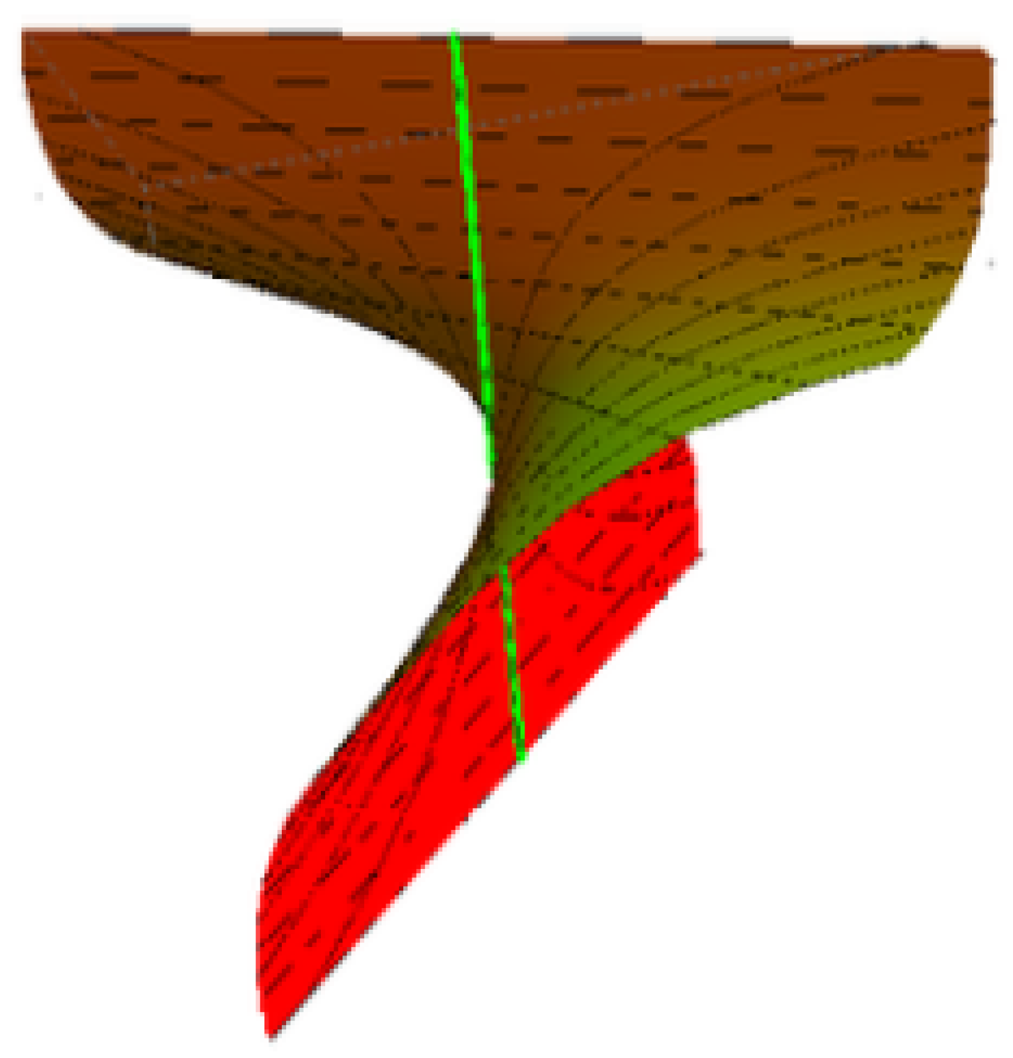
Example 1.

In what follows, we will construct the constant Disteli-axis timelike ruled surface $\left(X\right)$. Since $\widehat{\gamma }\left(\widehat{s}\right)$ is constant, from Equation (5), we obtain the ODE ${\widehat{\mathbf{t}}}^{{}^{{}^{″}}}-{\widehat{\kappa }}^2\widehat{\mathbf{t}}=\mathbf{0}$. Without loss of generality, assume $\widehat{\mathbf{t}}\left(0\right)=(0,1,0)$. The general solution of the ODE becomes

$$\widehat{\mathbf{t}}\left(\widehat{s}\right)=\left({\widehat{b}}_{1}sinh\widehat{\kappa }\widehat{s},cosh\widehat{\kappa }\widehat{s}+{\widehat{b}}_{2}sinh\widehat{\kappa }\widehat{s},{\widehat{b}}_{3}sinh\widehat{\kappa }\widehat{s}\right),$$

where ${\widehat{b}}_1$, ${\widehat{b}}_2$ and ${\widehat{b}}_3$ are dual constants. Since ${∥\widehat{\mathbf{t}}∥}^2=1$, we obtain ${\widehat{b}}_2=0$ and ${\widehat{b}}_1^2-{\widehat{b}}_3^2=1$. It follows that $\widehat{\mathbf{x}}\left(\widehat{s}\right)$ is given by

$$\widehat{\mathbf{x}}\left(\widehat{s}\right)=\left(\frac{{\widehat{b}}_1}{\widehat{\kappa }}cosh\widehat{\kappa }\widehat{s}+{\widehat{d}}_1,\frac{1}{\widehat{\kappa }}sinh\widehat{\kappa }\widehat{s},\frac{{\widehat{b}}_3}{\widehat{\kappa }}cosh\widehat{\kappa }\widehat{s}+{\widehat{d}}_3\right)$$

where ${\widehat{d}}_1$ and ${\widehat{d}}_3$ are dual constants, ${\widehat{b}}_1{\widehat{d}}_1-{\widehat{b}}_3{\widehat{d}}_3=0$, ${\widehat{d}}_3^2-{\widehat{d}}_1^2={\widehat{\rho }}^2-1$ and ${\widehat{\rho }}^2={cosh}^2\widehat{\psi }$. We now change the coordinates:

$$\left(\begin{array}{c}{\tilde{\widehat{x}}}_1\hfill \\ {\tilde{\widehat{x}}}_2\hfill \\ {\tilde{\widehat{x}}}_3\hfill \end{array}\right)=\left(\begin{array}{ccc}{\widehat{b}}_1\hfill & 0\hfill & -{\widehat{b}}_3\hfill \\ 0\hfill & 1\hfill & 0\hfill \\ -{\widehat{b}}_3\hfill & 0\hfill & {\widehat{b}}_1\hfill \end{array}\right)\left(\begin{array}{c}{\widehat{x}}_1\hfill \\ {\widehat{x}}_2\hfill \\ {\widehat{x}}_3\hfill \end{array}\right).$$

By the new coordinates ${\tilde{\widehat{x}}}_1,{\tilde{\widehat{x}}}_2$ and ${\tilde{\widehat{x}}}_3$, the dual unit vector $\widehat{\mathbf{x}}\left(\widehat{s}\right)$ becomes

$$\widehat{\mathbf{x}}\left(\widehat{\phi }\right)=\left(cosh\widehat{\psi }cosh\widehat{\phi },cosh\widehat{\psi }sinh\widehat{\phi },sinh\widehat{\psi }\right),$$

(31)

where $\widehat{\phi }=\widehat{\kappa }\widehat{s}$. It is a spacelike spherical curve with the dual curvature $\widehat{\kappa }=\sqrt{1-{\widehat{\gamma }}^2}$ on the hyperbolic dual unit sphere ${\mathbb{H}}_{+}^2$. Let $\widehat{\phi }=\phi (1+\epsilon h)$, h denoting the pitch of the screw motion. Then, Equation (31) represents a timelike ruled surface. Thus, the Blaschke frame is found as

$$\left(\begin{array}{c}\widehat{\mathbf{x}}\hfill \\ \widehat{\mathbf{t}}\hfill \\ \widehat{\mathbf{g}}\hfill \end{array}\right)=\left(\begin{array}{ccc}cosh\widehat{\psi }cosh\widehat{\phi }\hfill & cosh\widehat{\psi }sinh\widehat{\phi }\hfill & sinh\widehat{\psi }\hfill \\ sinh\widehat{\phi }\hfill & cosh\widehat{\phi }\hfill & 0\hfill \\ sinh\widehat{\psi }cosh\widehat{\phi }\hfill & sinh\widehat{\psi }sinh\widehat{\phi }\hfill & cosh\widehat{\psi }\hfill \end{array}\right)\left(\begin{array}{c}{\widehat{\mathbf{f}}}_1\hfill \\ {\widehat{\mathbf{f}}}_2\hfill \\ {\widehat{\mathbf{f}}}_3\hfill \end{array}\right).$$

(32)

It is easily seen from Equation (32) that

$$\left.\begin{array}{c}\hfill \widehat{p}\left(\phi \right)=(1+\epsilon h)cosh\widehat{\psi },\widehat{q}\left(\phi \right)=(1+\epsilon h)sinh\widehat{\psi },\\ \\ \hfill d\widehat{s}=\widehat{p}\left(\phi \right)d\phi ,\widehat{\gamma }\left(\phi \right)=:\frac{\widehat{q}\left(\phi \right)}{\widehat{p}\left(\phi \right)}=tanh\widehat{\psi }.\end{array}\right\}$$

(33)

From the real and dual parts of Equation (33), we find

$$\mu ={\psi }^{*}tanh\psi +h,\mathrm{and}\Gamma ={\psi }^{*}-htanh\psi .$$

(34)

Further, the Disteli-axis is

$$\widehat{\mathbf{b}}=sinh\widehat{\psi }\widehat{\mathbf{x}}-cosh\widehat{\psi }\widehat{\mathbf{g}}=-{\widehat{\mathbf{f}}}_3.$$

(35)

This means that $\left(X\right)$ is a constant Disteli-axis timelike ruled surface, that is, the axis of the helical motion is the constant Disetli-axis $\widehat{\mathbf{b}}$. Therefore, the equation of the base curve is the spacelike or timelike helix

$$\mathbf{c}\left(\phi \right)=\left({\psi }^{*}sinh\phi ,{\psi }^{*}cosh\phi ,-h\phi \right).$$

(36)

We can also show that if $\langle \frac{d\mathbf{c}\left(\phi \right)}{d\phi },\frac{d\mathbf{x}\left(\phi \right)}{d\phi }\rangle =0$, then the base curve $\mathbf{c}\left(\phi \right)$ of $\left(X\right)$ is its striction curve. Then, by means of the real part of Equation (31) and Equation (36), to the constant Disteli-axis timelike ruled surface $\left(X\right)$,

$$\mathbf{y}(\phi ,v):=\mathbf{c}\left(\phi \right)+v\mathbf{x}\left(\phi \right)=\left(\begin{array}{c}{\psi }^{*}sinh\phi +vcosh\psi cosh\phi \\ {\psi }^{*}cosh\phi +vcosh\psi sinh\phi \\ -h\phi +vsinh\psi \end{array}\right),v\in \mathbb{R},$$

(37)

where h, ψ and ${\psi }^{*}$ are constants. These constants can control the shape of $\left(X\right)$. Take $\psi ={\psi }^{*}=0$ and $h=-1$, for example. The timelike helicoidal surface is shown in Figure 2, where $-3\le \phi \le 3$ and $-1.5\le v\le 1.5$.

Example 2.

In this example, we verify the idea of Corollary 3. In view of Equations (24), (29), (32) and (33) we have that: $\widehat{\gamma }=tanh\widehat{\psi }=0$ ($\psi ={\psi }^{*}=0$)$\iff \widehat{\overline{\gamma }}+tanh\widehat{\vartheta }=0$ and

$$\widehat{\overline{\mathbf{x}}}\left(\widehat{\phi }\right)=\left(cosh\widehat{\vartheta }cosh\widehat{\phi },cosh\widehat{\vartheta }sinh\widehat{\phi },sinh\widehat{\vartheta }\right).$$

(38)

The equation of the striction curve of ($\overline{X}$), in terms of $\mathbf{c}\left(\phi \right)$, can therefore be written as:

$$\overline{\mathbf{c}}\left(\phi \right):=\mathbf{c}\left(\phi \right)+{\vartheta }^{*}\mathbf{t}\left(\phi \right)=\left(0,0,-h\phi \right)+{\vartheta }^{*}\left(sinh\phi ,cosh\phi ,0\right).$$

(39)

Then, we have the timelike Bertrand offset ($\overline{X}$)

$$\overline{\mathbf{y}}(\phi ,v):=\overline{\mathbf{c}}\left(\phi \right)+v\overline{\mathbf{x}}\left(\phi \right)=\left(\begin{array}{c}{\vartheta }^{*}sinh\phi +vcosh\vartheta cosh\phi \\ {\vartheta }^{*}cosh\phi +vcosh\vartheta sinh\phi ,\\ \overline{z}=-h\phi +vsinh\vartheta \end{array}\right),v\in \mathbb{R},$$

(40)

where h, ϑ and ${\vartheta }^{*}$ are constants. Take $\vartheta ={\vartheta }^{*}=1$ and $h=-10$, for example. The timelike Bertrand offset is shown in Figure 3, where $-3\le \phi \le 3$ and $-1.5\le v\le 1.5$. The graph of the timelike ruled surface $\left(X\right)$ with its Bertrand offset $\left(\overline{X}\right)$ is shown in Figure 4.

Properties of Striction Curves

With the aid of Definition 2, the striction curve $\overline{\mathbf{c}}\left(\overline{s}\right)$ of ($\overline{X}$) is obtained by

$$\overline{\mathbf{c}}\left(\overline{s}\right)=\mathbf{c}\left(s\right)+{\vartheta }^{*}\mathbf{t}\left(s\right),$$

(41)

from which we obtain

$$\frac{d\overline{\mathbf{c}}\left(\overline{s}\right)}{d\overline{s}}\frac{d\overline{s}}{ds}=(-\Gamma +{\vartheta }^{*})\mathbf{x}+(\mu +\gamma {\vartheta }^{*})\mathbf{g},$$

(42)

whereas, as in Equation (11), it is:

$$\frac{d\overline{\mathbf{c}}\left(\overline{s}\right)}{d\overline{s}}=-\overline{\Gamma }\left(\overline{s}\right)\overline{\mathbf{x}}\left(\overline{s}\right)+\overline{\mu }\left(\overline{s}\right)\overline{\mathbf{g}}\left(\overline{s}\right).$$

(43)

Thus, from Equations (42) and (43), we have

$$\frac{d\overline{s}}{ds}=\frac{-\Gamma +{\vartheta }^{*}}{-\overline{\Gamma }cosh\vartheta +\overline{\mu }sinh\vartheta }=\frac{\mu +\gamma {\vartheta }^{*}}{-\overline{\Gamma }sinh\vartheta +\overline{\mu }cosh\vartheta }.$$

(44)

If $\mu =0$, that is, if $\left(X\right)$ is the timelike tangent ruled surface of a given timelike space curve of class three, then, using Equation (44), it follows that

$$\overline{\mu }=\overline{\Gamma }\frac{\gamma {\vartheta }^{*}cosh\vartheta +\left(\Gamma -{\vartheta }^{*}\right)sinh\vartheta }{\gamma {\vartheta }^{*}sinh\vartheta +\left(\Gamma -{\vartheta }^{*}\right)cosh\vartheta }.$$

(45)

Thus, the Bertrand offset of a timelike tangential is not timelike tangential, that is, $\overline{\mu }\left(s\right)\ne 0$. If ($\overline{X}$) is also a timelike tangential, that is, $\overline{\mu }\left(s\right)=0$, then we obtain the relation

$$\left(1-{\vartheta }^{*}\kappa \left(u\right)\right)sinh\vartheta +{\vartheta }^{*}\tau \left(u\right)cosh\vartheta =0.$$

(46)

Corollary 6.

If $\left(X\right)$ and $\left(\overline{X}\right)$ are two timelike tangential Bertrand offsets, then their striction curves are timelike Bertrand curves.

Furthermore, from Equation (46), the offset distance ${\vartheta }^{*}$ is

$${\vartheta }^{*}=\frac{sinh\vartheta }{\kappa \left(u\right)sinh\vartheta -\tau \left(u\right)cosh\vartheta }.$$

(47)

Hence, when the timelike tangential offset of a timelike tangential surface is an oriented offset, then it is a coincident offset. If a timelike plane curve $\tau \left(u\right)=0$, in view of Equation (46), it leads to $\kappa \left(u\right)$ being constant. Here, $\overline{\mathbf{c}}\left(u\right)=\overline{\mathbf{c}}\left(u\right)$, and $\mathbf{c}\left(u\right)$ is closed and self-mated. In addition, Equation (41) becomes

$$\overline{\mathbf{c}}\left(u\right)=\mathbf{c}\left(u\right)+{\vartheta }^{*}{\zeta }_2\left(u\right).$$

(48)

From the fact that ${∥{\zeta }_2∥}^2=1$, we obtain:

$${∥\overline{\mathbf{c}}\left(u\right)-\mathbf{c}\left(u\right)∥}^2={\vartheta }^{*2}>0.$$

Corollary 7.

Every closed self-mated timelike tangential surface has constant width.

When $\Gamma =0$, the surface (X) is a timelike binormal ruled surface of its timelike striction curve. From Equation (44), it follows that

$$\overline{\Gamma }=\overline{\mu }\frac{{\vartheta }^{*}cosh\vartheta -\left(\gamma {\vartheta }^{*}+\mu \right)sinh\vartheta }{{\vartheta }^{*}sinh\vartheta -\left(\gamma {\vartheta }^{*}+\mu \right)cosh\vartheta }.$$

(49)

Thus, the Bertrand offset of a timelike binormal is not timelike binormal, that is, $\overline{\Gamma }\left(s\right)\ne 0$. Furthermore, if the timelike Bertrand offset ($\overline{X}$) is also timelike binormal, then we have:

$$\tau \left(u\right){\vartheta }^{*}cosh\vartheta -\left(\kappa \left(u\right){\vartheta }^{*}+1\right)sinh\vartheta =0.$$

In similar arguments, we can give the corresponding results for a timelike tangential. We omit the details here.

4. Conclusions

In this paper, a generalization of Bertrand offsets of curves for timelike ruled surfaces has been developed. Interestingly, there are many similarities between the theory of Bertrand curves and the theory of Bertrand offsets for timelike ruled surfaces. For instance, a timelike ruled surface can have an infinity of Bertrand offsets in the same way as a plane curve can have an infinity of Bertrand mates. Moreover, in recent years, the study of singularity theory, submanifolds theory, harmonic quasiconformal mappings, etc. are significant fields of modern mathematical research. Most researchers have paid more attention to cross-disciplinary research, which is a new trend and a promising direction. It is suggested that Gaussian and mean curvatures of these Bertrand offsets can be calculated when the Weingarten map for the Bertrand offsets’ spacelike ruled surfaces is determined. Moreover, connecting the study of singularity theory and submanifolds theory presented in [23,24,25,26,27,28,29,30,31,32,33,34,35,36] can be considered to explore new methods to obtain more results and theorems related to symmetric properties about this topic.

References

1. Bottema, O.; Roth, B. Theoretical Kinematics; North-Holland Press: New York, NY, USA, 1979. [Google Scholar]
2. Karger, A.; Novak, J. Space Kinematics and Lie Groups; Gordon and Breach Science Publishers: New York, NY, USA, 1985. [Google Scholar]
3. Pottman, H.; Wallner, J. Computational Line Geometry; Springer: Berlin/Heidelberg, Germany, 2001. [Google Scholar]
4. Ravani, B.; Ku, T.S. Bertrand offsets of ruled and developable surfaces. Comput. Aided Des. 1991, 23, 145–152. [Google Scholar] [CrossRef]
5. Küçük, A.; Gürsoy, O. On the invariants of Bertrand trajectory surface offsets. Appl. Math. Comput. 2004, 151, 763–773. [Google Scholar] [CrossRef]
6. Kasap, E.; Kuruoglu, N. Integral invariants of the pairs of the Bertrand ruled surface. Bull. Pure Appl. Sci. Sect. E Math. 2002, 21, 37–44. [Google Scholar]
7. Kasap, E.; Kuruoglu, N. The Bertrand offsets of ruled surfaces in R 1 3 . Acta Math. Vietnam 2006, 31, 39–48. [Google Scholar]
8. Kasap, E.; Yuce, S.; Kuruoglu, N. The involute-evolute offsets of ruled surfaces. Iranian J. Sci. Tech. Trans. A 2009, 33, 195–201. [Google Scholar]
9. Orbay, K.; Kasap, E.; Aydemir, I. Mannheim offsets of ruled surfaces. Math. Probl. Eng. 2009, 2009, 160917. [Google Scholar] [CrossRef]
10. Onder, M.; Ugurlu, H.H. Frenet frames and invariants of timelike ruled surfaces. Ain. Shams Eng. J. 2013, 4, 507–513. [Google Scholar] [CrossRef] [Green Version]
11. Sentrk, G.Y.; Yuce, S. Properties of integral invariants of the involute-evolute offsets of ruled surfaces. Int. J. Pure Appl. Math. 2015, 102, 757–768. [Google Scholar] [CrossRef]
12. Aldossary, M.T.; Abdel-Baky, R.A. On the Bertrand offsets for ruled and developable surfaces. Boll. Unione Mat. Ital. 2015, 8, 53–64. [Google Scholar] [CrossRef]
13. Sentrk, G.Y.; Yuce, S.; Kasap, E. Integral Invariants of Mannheim offsets of ruled surfaces. Appl. Math. E-Notes 2016, 16, 198–209. [Google Scholar]
14. Sentrk, G.Y.; Yuce, S. Bertrand offsets of ruled surfaces with Darboux frame. Results Math. 2017, 72, 1151–1159. [Google Scholar] [CrossRef]
15. Sentrk, G.Y.; Yuce, S. On the evolute offsets of ruled surfaces using the Darboux frame. Commun. Fac. Sci. Univ. Ank. Ser. A1 Math. Stat. 2019, 68, 1256–1264. [Google Scholar]
16. Önder, M. Darboux Approach to Bertrand Surface Offsets. Int. J. Pure App. (IJPAM) 2011, 74, 221–234. [Google Scholar]
17. Abdel-Baky, R.A.; Unluturk, Y. A new construction of timelike ruled surfaces with constant Disteli-axis. Honam Math. J. 2020, 42, 551–568. [Google Scholar]
18. O’Neil, B. Semi-Riemannian Geometry Geometry, with Applications to Relativity; Academic Press: New York, NY, USA, 1983. [Google Scholar]
19. Walfare, J. Curves and Surfaces in Minkowski Space. Ph.D. Thesis, K.U. Leuven, Faculty of Science, Leuven, Belgium, 1995. [Google Scholar]
20. Pottmann, H. Holditch-Sicheln. Arch. Math. 1985, 44, 373–378. [Google Scholar]
21. Hascisalihoglu, H.H.; Abdel-Baky, R.A. Holditch’s theorem for one-parameter closed motions. Mech. Mach. Theory 1997, 32, 235–239. [Google Scholar] [CrossRef]
22. Pekmen, U.; Pasali, S. Some characterizations of Lorentzian spherical spacelike curves. Math. Morav. 1999, 3, 31–37. [Google Scholar]
23. Li, Y.L.; Liu, S.Y.; Wang, Z.G. Tangent developables and Darboux developables of framed curves. Topol. Appl. 2021, 301, 107526. [Google Scholar] [CrossRef]
24. Li, Y.L.; Wang, Z.G. Lightlike tangent developables in de Sitter 3-space. J. Geom. Phys. 2021, 164, 1–11. [Google Scholar] [CrossRef]
25. Li, Y.L.; Wang, Z.G.; Zhao, T.H. Geometric Algebra of Singular Ruled Surfaces. Adv. Appl. Clifford Algebras. 2021, 31, 1–19. [Google Scholar] [CrossRef]
26. Li, Y.L.; Zhu, Y.S.; Sun, Q.Y. Singularities and dualities of pedal curves in pseudo-hyperbolic and de Sitter space. Int. J. Geom. Methods Mod. Phys. 2021, 18, 1–31. [Google Scholar] [CrossRef]
27. Li, Y.L.; Ganguly, D.; Dey, S.; Bhattacharyya, A. Conformal η-Ricci solitons within the framework of indefinite Kenmotsu manifolds. AIMS Math. 2022, 7, 5408–5430. [Google Scholar] [CrossRef]
28. Li, Y.L.; Alkhaldi, A.H.; Ali, A.; Laurian-Ioan, P. On the Topology of Warped Product Pointwise Semi-Slant Submanifolds with Positive Curvature. Mathematics 2021, 9, 3156. [Google Scholar] [CrossRef]
29. Li, Y.L.; Lone, M.A.; Wani, U.A. Biharmonic submanifolds of Kähler product manifolds. AIMS Math. 2021, 6, 9309–9321. [Google Scholar] [CrossRef]
30. Li, Y.L.; Ali, A.; Ali, R. A general inequality for CR-warped products in generalized Sasakian space form and its applications. Adv. Math. Phys. 2021, 2021, 5777554. [Google Scholar] [CrossRef]
31. Li, Y.L.; Ali, A.; Mofarreh, F.; Abolarinwa, A.; Ali, R. Some eigenvalues estimate for the ϕ-Laplace operator on slant submanifolds of Sasakian space forms. J. Funct. Space 2021, 2021, 6195939. [Google Scholar]
32. Li, Y.L.; Ali, A.; Mofarreh, F.; Alluhaibi, N. Homology groups in warped product submanifolds in hyperbolic spaces. J. Math. 2021, 2021, 8554738. [Google Scholar] [CrossRef]
33. Yang, Z.C.; Li, Y.L.; Erdoǧdub, M.; Zhu, Y.S. Evolving evolutoids and pedaloids from viewpoints of envelope and singularity theory in Minkowski plane. J. Geom. Phys. 2022, 2022, 104513. [Google Scholar] [CrossRef]
34. Todorčević, V. Harmonic Quasiconformal Mappings and Hyperbolic Type Metrics; Springer: Berlin/Heidelberg, Germany, 2019. [Google Scholar]
35. Todorčević, V. Subharmonic behavior and quasiconformal mappings. Anal. Math. Phys. 2019, 9, 1211–1225. [Google Scholar] [CrossRef]
36. Debnath, P.; Konwar, N.; Radenovic, S. Metric fixed Point Theory: Applications in Science. In Engineering and Behavioural Sciences; Springer Nature: Singapore, 2021. [Google Scholar]
Figure 1. The dual hyperbolic and dual Lorentzian unit spheres.
Symmetry 14 00783 g001
Figure 2. Timelike helicoidal surface.
Symmetry 14 00783 g002
Figure 3. Timelike Bertrand offset.
Symmetry 14 00783 g003
Figure 4. ( X ) and its Bertrand offset ( X ¯ ).
Symmetry 14 00783 g004
Publisher’s Note: MDPI stays neutral with regard to jurisdictional claims in published maps and institutional affiliations.