Compensation of the Frequency Offset in Communication Systems with LoRa Modulation

Abstract

This study focused on methods estimation and compensation frequency offset in communication systems with LoRa modulation. LoRa being used in IoT applications rapidly expands its markets. The article discusses three methods for estimation and compensation frequency offset as well as details of the comparative analysis made. Aside from the well-known methods by Ghanaatian and Golden Section Search (GSS), the third method is offered by the authors of the article and represents an improved version of the method proposed by Ghanaatian. The proposed method is based on a symmetric processing signal that is divided into two parts. The advantages and drawbacks of the considered methods are described. As a result of the performed study, a software model was developed, the dependence of the root mean-square error (RMSE) estimation of the frequency offset, and cumulative density function (CDF) of the frequency estimation error was calculated. Modeling was performed under identical conditions. The frequency offset accuracy provided by the proposed method exceeded the accuracy of the considered methods.

1. Introduction

Internet of Things (IoT) is the connection of network-enabled devices and recently, it also refers to the value-chain created by connecting things, data, humans, and services. IoT devices are accumulator-operated and it is crucial to keep all of the sensors and other devices connected to the network. This situation is also required for new economic-efficient solutions such as low-power wide area networks (LPWANs).

LPWANs determine the category of wireless communications technology, which recently acquired a significant impulse and has been the subject of much modern research work [1,2]. Organizations in the development of industry, academies, and standards have devoted significant efforts on LPWANs in recent years [3]. Such technologies usually offer a communication range within several kilometers where one gateway supports thousands of devices such as sensors [4]. Consequently, LPWAN technology includes IoT applications such as smart homes or cities due to its low cost. Among the LPWAN technologies, LoRaWAN and LoRa (long range) modulation (used in this LoRaWAN protocol) are the technologies that have captured significant attention from the modern scientific sector, which is reflected in the following works [5,6,7]. This fact can be explained as follows: the open access specification [8]; the availability of certified equipment [9]; simplified process of establishment connections and low power consumption [10,11], which is extremely important for IoT devices.

LoRa is a recent technology related to the LPWAN and is created by the Semtech company, and is also one of the most popular protocols for IoT systems, where the linear frequency modulation (LFM) is applied. LoRa provides scaling of the time-bandwidth product and has low power consumption. Aside from IoT systems, the LFM modulation is applied to communicate with unmanned aerial vehicles (UAVs) [12], power line communications [13], and satellite communications [14,15]. In such communication systems, developers are forced to increase the duration of the signals to fight against negative effects and increase the communication range. Large signal duration makes it more vulnerable to frequency offset [16].

When considering methods, these can be divided into two categories. The first category includes methods based on the calculation of the phase difference between the reference signal and the test signal. The second category includes methods based on the calculation of the maximum likelihood function [17] (MLF). The first category of method estimation accuracy is limited by phase calculation algorithms. The second category of methods are reliable and high-precision but have large computational costs when considering the large sample length.

The obtained results could be useful for developers of satellite communication systems, radar, and IoT systems.

This article is arranged as follows. In Section 2, the considering methods and LoRa background are described. Section 3 explains the modeling and experimental results and Section 4 concludes the outcomes of this article.

2. LoRa Background

In LoRa, LFM signals are used and called chirps [18,19]. There are two types of chirps, the first type has an increasing frequency—upchirp, and the second type has a decreasing frequency—downchirp. Chirp signals have large time-bandwidth products. The main parameters of the chirps according to the LoRa specification [20] are as follows:

• Signal bandwidth, $BW=125,250,500$ kHz;
• Spreading factor, $SF=7,8,9,10,11,12$;
• Symbol duration, $Ts=2^{SF}/BW$; and
• number of the preamble symbols, $N=8$.

The unmodulated chirp is described by the following expression [21,22]:

$$X[n]=\frac{1}{\sqrt{2^{SF}}}\exp \left(\frac{j\cdot \pi \cdot n^2}{2^{SF}}\right);n=1\dots 2^{SF}$$

(1)

where $\frac{1}{\sqrt{2^{SF}}}$ is a scale coefficient.

Modulation performing is as follows [23,24]: $SF$ bits are selected from the information bit stream and converted into a decimal number system. As a result, the bit is transformed into a decimal information number within $K=0\dots 2^{SF}-1$. Then, the modulated chirp can be written as:

$$Y[n]=\frac{1}{\sqrt{2^{SF}}}\exp \left(j\cdot \pi \cdot (n^2+2\cdot K\cdot n)\cdot \frac{1}{2^{SF}}\right);n=1\dots 2^{SF}$$

(2)

When demodulating, the input chirp is multiplied by the complex-conjugate unmodulated chirp. The fast Fourier transform (FFT) is applied for the multiplication result. Then, the search of the sample number corresponding to the maximum spectrum value must be performed:

$$K=\max \langle \mathrm{FFT}\left(Y\left[n\right]\cdot X^{*}\left[n\right]\right)\rangle$$

(3)

Afterward, the obtained information number is converted into a binary system to obtain a demodulated bit sequence.

In [1], the two-stage method for estimation and compensation frequency offset is proposed. In the first stage, the coarse estimation is performed. In the second stage, the fine estimation is carried out. A coarse estimation process is based on the demodulation procedure. Since the preamble does not consist of modulated chirps, it is used for the estimation process. The fine estimation is performed by calculating the phase difference between the two adjoined chirps.

The received preamble chirps are multiplied by the reference chirp (unmodulated complex-conjugate chirp) and for the result of the multiplication, FFT is calculated using Equation (4). Then, the spectrum peak search and calculating information symbol value $K$ is performed. For the preamble chirps, the information symbol equals 0. In the presence of frequency offset, the information symbol value will differ from 0. The chirp consists of $2^{SF}$ samples, the frequency interval between the samples will depend on $SF$ and $BW$, then its value is equal to $f_{\mathrm{SAMP}}=BW/2^{SF}$. Therefore, to calculate the frequency offset, the demodulated value of the information symbol $K$ is multiplied by $f_{\mathrm{SAMP}}$ (4).

$$\left[{\widehat{f}}_1,{\widehat{f}}_2,\dots {\widehat{f}}_N\right]=f_{\mathrm{SAMP}}\cdot \left\{\max \langle \mathrm{FFT}\left(Y_i\left[n\right]\cdot X^{*}\left[n\right]\right)\rangle \right\},n=1\dots 2^{SF}$$

(4)

where $i$ is a preamble symbol number;

$\mathrm{FFT}$ is the fast Fourier transform;

$Y_i\left[n\right]$ are the received preamble chirps;

$X^{*}\left[n\right]$ is a reference chirp (complex-conjugate unmodulated chirp (1)); and

${\widehat{f}}_1,{\widehat{f}}_2,\dots {\widehat{f}}_N\in f_{\mathrm{SAMP}}\cdot \left[0\dots 2^{SF}-1\right]$ is a coarse frequency offset estimation calculated for each preamble symbol.

Then, the averaging of the calculated estimations is performed:

$$\Delta {\widehat{f}}_{\mathrm{COARSE}}=\frac{{\widehat{f}}_1+{\widehat{f}}_2+\dots {\widehat{f}}_N}{N}$$

(5)

where $N$ is a number of transmitted preamble symbols.

Functional diagram of the coarse estimation process is presented in Figure 1.

When performing a coarse estimation, the maximum error of the frequency offset estimation is equal to $f_{\mathrm{FRAQ}\text{\_}\mathrm{MAX}}=f_{\mathrm{SAMP}}/2$. Therefore, frequency error estimation is within the $\left[-f_{\mathrm{FRAQ}\text{\_}\mathrm{MAX}}:+f_{\mathrm{FRAQ}\text{\_}\mathrm{MAX}}\right]$ Hz sweep. Residual frequency offset close enough to $\left(f_{\mathrm{SAMP}}\cdot m\right)/2;m=1,3,5,7,\dots ,SF-1$ leads to demodulation errors and additional compensation operation is needed.

After performing coarse estimation, the frequency offset compensation can be expressed as follows in Equation (6).

$${\tilde{\mathbf{Y}}}_{\mathrm{COARSE},i}\left[n\right]=Y_i\left[n\right]\cdot e^{j\cdot 2\cdot \pi \cdot n\left(\frac{\Delta {\widehat{f}}_{\mathrm{COARSE}}}{f_{\mathrm{SR}}}\right)}$$

(6)

where $f_{\mathrm{SR}}$ is a sampling frequency (sample rate); and

${\tilde{\mathbf{Y}}}_{\mathrm{COARSE},i}\left[n\right]$ chirps after coarse estimation and compensation frequency offset.

The frequency offset leads to phase offset between two adjoint chirps. This feature is used in the Ghanaatian method to perform the fine estimation. Between two adjoint chirps in the preamble, the phase offset can be calculated as:

$$\Delta \Phi =\arg \langle {\displaystyle \sum _{n=1}^{2^{SF}}Y\left[n\right]\cdot Y^{*}\left[n+2^{SF}\right]}\rangle$$

(7)

where $\Delta \Phi$ is a phase offset between two adjoint chirps.

Operation (7) is performed between all chirps in the preamble, then the average estimation is calculated:

$$\Delta \overline{\Phi }=\frac{\Delta {\Phi }_1+\Delta {\Phi }_2+\dots \Delta {\Phi }_N}{N}$$

(8)

The obtained phase offset estimation can be used to calculate the frequency offset:

$$\Delta {\widehat{f}}_{\mathrm{FINE}}=\frac{\Delta \overline{\Phi }}{2\cdot \pi \cdot Ts}$$

(9)

where $\Delta {\widehat{f}}_{\mathrm{FINE}}$ is a fine frequency offset estimation.

Functional diagram of the fine estimation process is presented in Figure 2.

The resulting frequency offset estimation is equal to:

$$\Delta {\widehat{f}}_{\mathrm{EST}}=\Delta {\widehat{f}}_{\mathrm{COARSE}}+\Delta {\widehat{f}}_{\mathrm{FINE}}$$

(10)

The frequency offset compensation can be performed as:

$${\tilde{\mathbf{Y}}}_{\mathrm{FINE},i}\left[n\right]={\tilde{\mathbf{Y}}}_{\mathrm{COARSE},i}\left[n\right]\cdot e^{j\cdot 2\cdot \pi \cdot n\left(\frac{\Delta {\widehat{f}}_{\mathrm{EST}}}{f_{\mathrm{SR}}}\right)}$$

(11)

where ${\tilde{\mathbf{Y}}}_{\mathrm{FINE},i}\left[n\right]$ represents chirps after fine estimation and compensation frequency offset.

Considering the GSS method allows one to calculate the fine frequency offset estimation where an iterative mathematical algorithm GSS is applied to find the extremum of the MLF. It is assumed that a coarse estimation is performed using the Ghanaatian method [2].

First, one needs to define the unmodulated chirp (2) consisting frequency offset:

$$Y_{\mathrm{OFFSET}}\left[n\right]=\frac{1}{\sqrt{2^{SF}}}{e}^{j\cdot \pi \cdot \frac{n^2}{2^{SF}}}\cdot e^{j\cdot 2\cdot \pi \cdot \frac{\Delta f\cdot (n+i\cdot 2^{SF})}{BW}},n=1\dots 2^{SF}$$

(12)

where $\Delta f$ is a frequency offset.

The second exponential component in expression (12) defines the frequency offset. The result of multiplying the input chirps by this component, having the opposite sign, will be the compensated frequency offset chirp:

$$Z_i\left[n\right]=Y_{\mathrm{OFFSET},i}\left[n\right]\cdot W\left[n\right],n=1\dots 2^{SF}$$

(13)

where $Z\left[n\right]$ is a compensated frequency offset chirp; and

$W\left[n\right]$ is the frequency offset component with opposite sign.

$$W\left[n\right]=e^{-j\cdot 2\cdot \pi \cdot \frac{\Delta f^{\prime }\cdot (n+i\cdot 2^{SF})}{BW}}n=1\dots 2^{SF}$$

(14)

where $\Delta f^{\prime }$ is the compensated frequency offset value.

The compensated frequency offset chirp (13) is multiplied by unmodulated complex-conjugate chirp, then all samples are modulo addition. The obtained result is the number in the range $0\dots 1$ (this is due to scale coefficient in expression (1)).

$$\left|{\displaystyle \sum \left(Z_i\left[n\right]\cdot X^{*}\left[n\right]\right)}\right|=0\dots 1$$

(15)

The calculation (15) for all possible residual frequency offsets is the MLF (16). MLF has the maximum value when $\Delta f$ equals $\Delta f^{\prime }$.

$${\mathrm{R}}_i\left(\Delta F_{\mathrm{DIFF}}\right)=\mathrm{R}(\Delta f-\Delta f^{\prime })=\left|{\displaystyle \sum \left(Z_i\left[n\right]\cdot X^{*}\left[n\right]\right)}\right|$$

(16)

where $\Delta F_{\mathrm{DIFF}}$ is a frequency offset estimation error;

${\mathrm{R}}_i\left(\Delta F_{\mathrm{DIFF}}\right)\in 0\dots 1$ is the maximum likelihood function; and

$\Delta f^{\prime }\in -{\mathrm{F}}_{\mathrm{X}}\dots +{\mathrm{F}}_{\mathrm{X}}$ is the sweep of the residual frequency offset.

Figure 3, Figure 4 and Figure 5 show the function $\mathrm{R}\left(\Delta F_{\mathrm{DIFF}}\right)$ for cases when frequency offset in the input chirp are equal to $+{\mathrm{F}}_{\mathrm{X}}$ Hz, $-{\mathrm{F}}_{\mathrm{X}}$ Hz and 0 Hz, respectively. Functional diagram of the GSS method is presented in Figure 6. Note that in the absence of the frequency offset, the MLF has a symmetric shape (Figure 5).

The use of the GSS method allows one to quickly find the extremum of MLF (16) and does not require computations to be performed for all residual frequency offsets [25]. An example of GSS functioning is shown in Figure 7. The description for the GSS method is given below in Figure 7.

Furthermore, the execution of the first iteration is given. In the range ${\mathrm{A}}_i$ and ${\mathrm{D}}_i$, the point ${\mathrm{B}}_i$ is chosen in such a way that the ratio of the intervals $[{\mathrm{B}}_i:{\mathrm{D}}_i]$ and $[{\mathrm{A}}_i:{\mathrm{B}}_i]$ is equal to the proportion of the golden section 1.618. Similar to point ${\mathrm{B}}_i$, the position of point ${\mathrm{C}}_i$ is calculated (detailed formulas for calculating are given in [2]). At points ${\mathrm{B}}_i$ and ${\mathrm{C}}_i$ the value of the function (16) is calculated:

$$\begin{array}{l}{\mathrm{R}}_{1,i}\left(\Delta F_{\mathrm{DIFF}}\right)={\mathrm{R}}_{1,i}(\Delta f-{\mathrm{B}}_i)=\left|{\displaystyle \sum \left(Z_{1,i}\left[n\right]\cdot X_i^{*}\left[n\right]\right)}\right|;\\ {\mathrm{R}}_{2,i}\left(\Delta F_{\mathrm{DIFF}}\right)={\mathrm{R}}_{2,i}(\Delta f-{\mathrm{C}}_i)=\left|{\displaystyle \sum \left(Z_{2,i}\left[n\right]\cdot X_i^{*}\left[n\right]\right)}\right|.\end{array}$$

(17)

where $Z_{1,i}\left[n\right]$ is a compensated frequency offset chirp for the point ${\mathrm{B}}_i$;

$Z_{2,i}\left[n\right]$ is the compensated frequency offset chirp for the point ${\mathrm{C}}_i$;

${\mathrm{R}}_{1,i}\left(\Delta F_{\mathrm{DIFF}}\right)$ is the MLF for point ${\mathrm{B}}_i$; and

${\mathrm{R}}_{2,i}\left(\Delta F_{\mathrm{DIFF}}\right)$ is the MLF for point ${\mathrm{C}}_i$.

Thus, the arguments for calculating the MLF are selected symmetrically relative to the considered interval $[{\mathrm{A}}_i:{\mathrm{D}}_i]$.

After calculating (17), ${\mathrm{R}}_1\left(\Delta F_{\mathrm{DIFF}}\right)$ is compared to ${\mathrm{R}}_2\left(\Delta F_{\mathrm{DIFF}}\right)$. Then, a new interval for search extremum MLF is selected. This interval is also divided into proportion of the golden section, as described above, but the calculation of the function value is performed only at one point, since one value of the function is known from the previous iteration. For example, if ${\mathrm{R}}_1\left(\Delta F_{\mathrm{DIFF}}\right)$ is greater than ${\mathrm{R}}_2\left(\Delta F_{\mathrm{DIFF}}\right)$, then the new interval is defined as follows:

• ${\mathrm{A}}_{i+1}={\mathrm{A}}_i$;
• ${\mathrm{B}}_{i+1}$ is chosen in such a way that the ratio $[{\mathrm{B}}_i:{\mathrm{D}}_i]/[{\mathrm{A}}_i:{\mathrm{B}}_i]=1.618$;
• ${\mathrm{C}}_{i+1}={\mathrm{B}}_i$; and
• ${\mathrm{D}}_{i+1}={\mathrm{C}}_i$.

In the results, points $\mathrm{B}$ and $\mathrm{C}$ form the interval, where the extremum of the MLF is located. The length of this interval is determined by setting the accuracy.

As can be seen, frequency estimation error of the GSS method is defined by the accuracy and approximate value of the ratio of the golden section. However, at the same time, the method provides a quick search for extremum MLF.

The frequency offset compensation can be performed as in expressions (13) and (14).

The proposed method is an improved version of the Ghanaatian method. Before performing the fine estimation (9), an additional frequency offset estimation is applied using half of the chirps.

The need for an additional estimation is conditioned by the fact that the frequency offsets that are close in magnitude to the $\left(f_{\mathrm{SAMP}}\cdot m\right)/2$, especially when the SNR is low (0 dB), so it is not always possible to perform estimation correctly, since there is a sign ambiguity of the frequency estimation. It can lead to the large frequency estimation errors due to the correct estimation of the magnitude, but the incorrect sign.

This occurs because the $\arg$ function (used in fine frequency estimation) returns the phase offset value in the interval $\left[-\pi :\pi \right]$ [26]. When noise power is high, the $\arg$ function can work incorrectly. LoRa technology can provide robust communication, even in the presence of high noise level [27]. After the coarse estimation, the residual offset can be significantly compensated by performing additional estimation. Therefore, fine estimation can be performed correctly.

The received preamble chirp (1) and the reference chirp (complex-conjugate (1)) are divided into two equal parts:

$$\begin{array}{l}\{\begin{array}{c}{y}_1\left[m\right]=Y\left[m\right];\\ x_1^{*}\left[m\right]=X^{*}\left[m\right];\end{array}m=1\dots \frac{2^{SF}}{2}\\ \{\begin{array}{c}{y}_2\left[k\right]=Y\left[k\right];\\ x_2^{*}\left[k\right]=X^{*}\left[k\right];\end{array}k=\frac{2^{SF}}{2}+1\dots 2^{SF}\end{array}$$

(18)

The $y_1\left[m\right]$ component of the received chirp is multiplied by the component $x_1^{*}\left[m\right]$ of the reference chirp, and respectively $y_2\left[k\right]$ is multiplied by $x_2^{*}\left[k\right]$:

$$\begin{array}{l}{z}_1\left[m\right]=y_1\left[m\right]\cdot x_1^{*}\left[m\right];\\ z_2\left[k\right]=y_2\left[k\right]\cdot x_2^{*}\left[k\right];\end{array}$$

(19)

Furthermore, the results of the multiplication (19) FFT can be calculated in the following way:

$$\begin{array}{l}{z}_1\left[w\right]=\mathrm{FFT}\left(z_1\left[m\right]\right);\\ z_2\left[w\right]=\mathrm{FFT}\left(z_2\left[k\right]\right);\end{array}$$

(20)

where $z_1\left[w\right]$ and $z_2\left[w\right]$ is a multiplication spectrum (19).

Furthermore, the search for the maximum value of the spectrum is performed, then the $\arg$ function is calculated for this value. Its operations are performed for components $y_1\left[m\right]$ and $y_2\left[k\right]$.

$$\begin{array}{l}\Delta {\varphi }_1=\arg \langle \max \left(\left|z_1\left[w\right]\right|\right)\rangle ;\\ \Delta {\varphi }_2=\arg \langle \max \left(\left|z_2\left[w\right]\right|\right)\rangle ;\end{array}$$

(21)

where $\Delta {\varphi }_1$ is a phase offset in the $y_1\left[m\right]$ component; and

$\Delta {\varphi }_2$ is the phase offset in the $y_2\left[k\right]$ component.

The result of the subtraction component from expression (21) can be used to calculate the full phase frequency offset.

$$\Delta {\widehat{f}}_{\mathrm{EST}\text{\_}\mathrm{EXTRA}}=\frac{\Delta {\varphi }_2-\Delta {\varphi }_1}{\pi \cdot Ts}$$

(22)

Functional diagram of the proposed method is shown in Figure 8. As can be seen from Figure 8, the functional diagram of the proposed method has a symmetric structure.

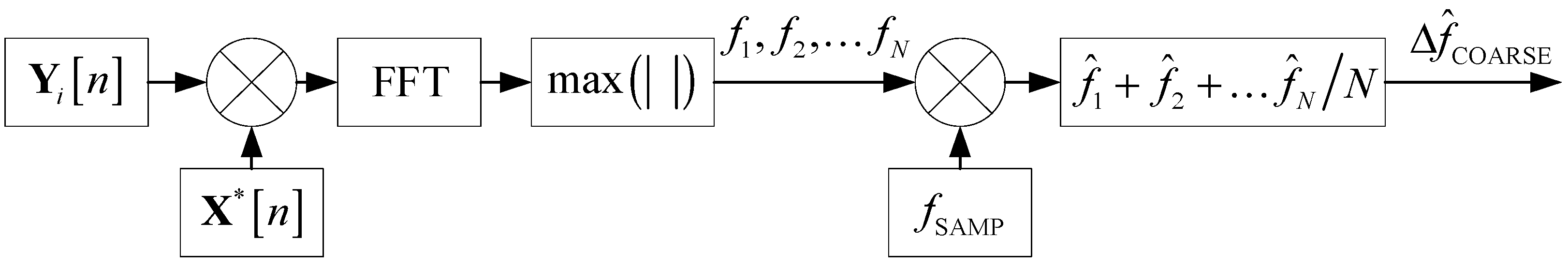
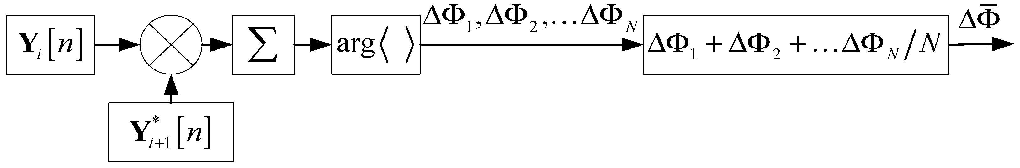
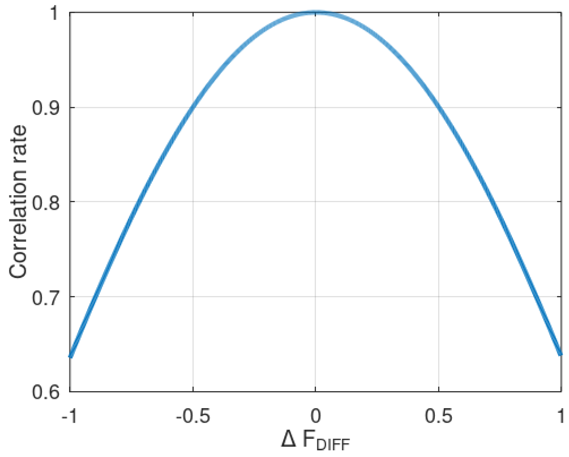
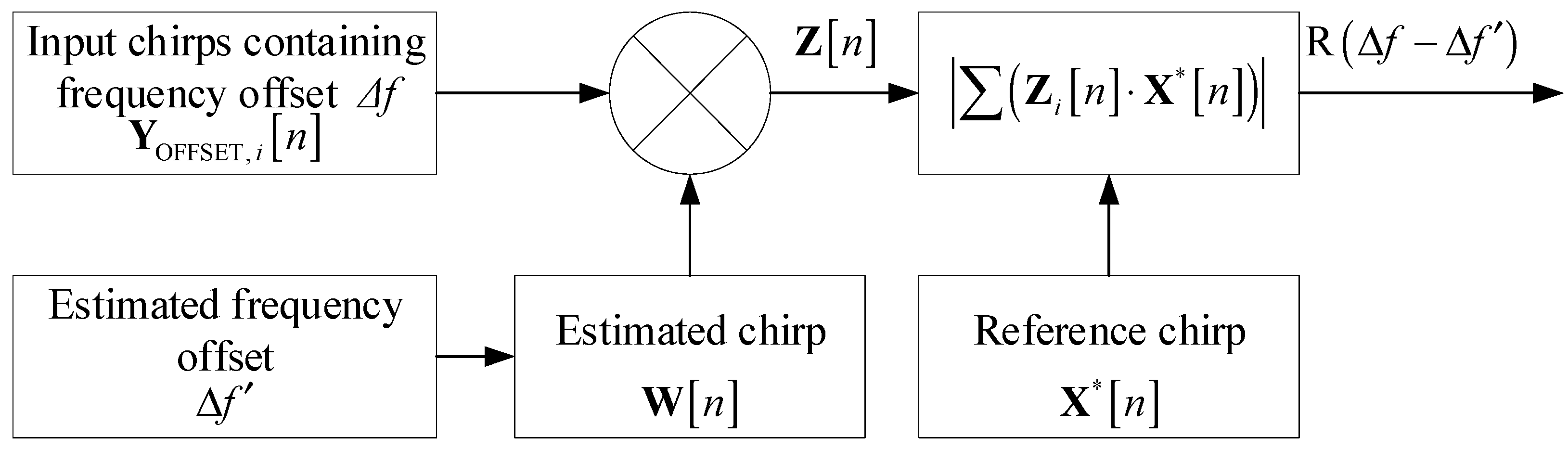
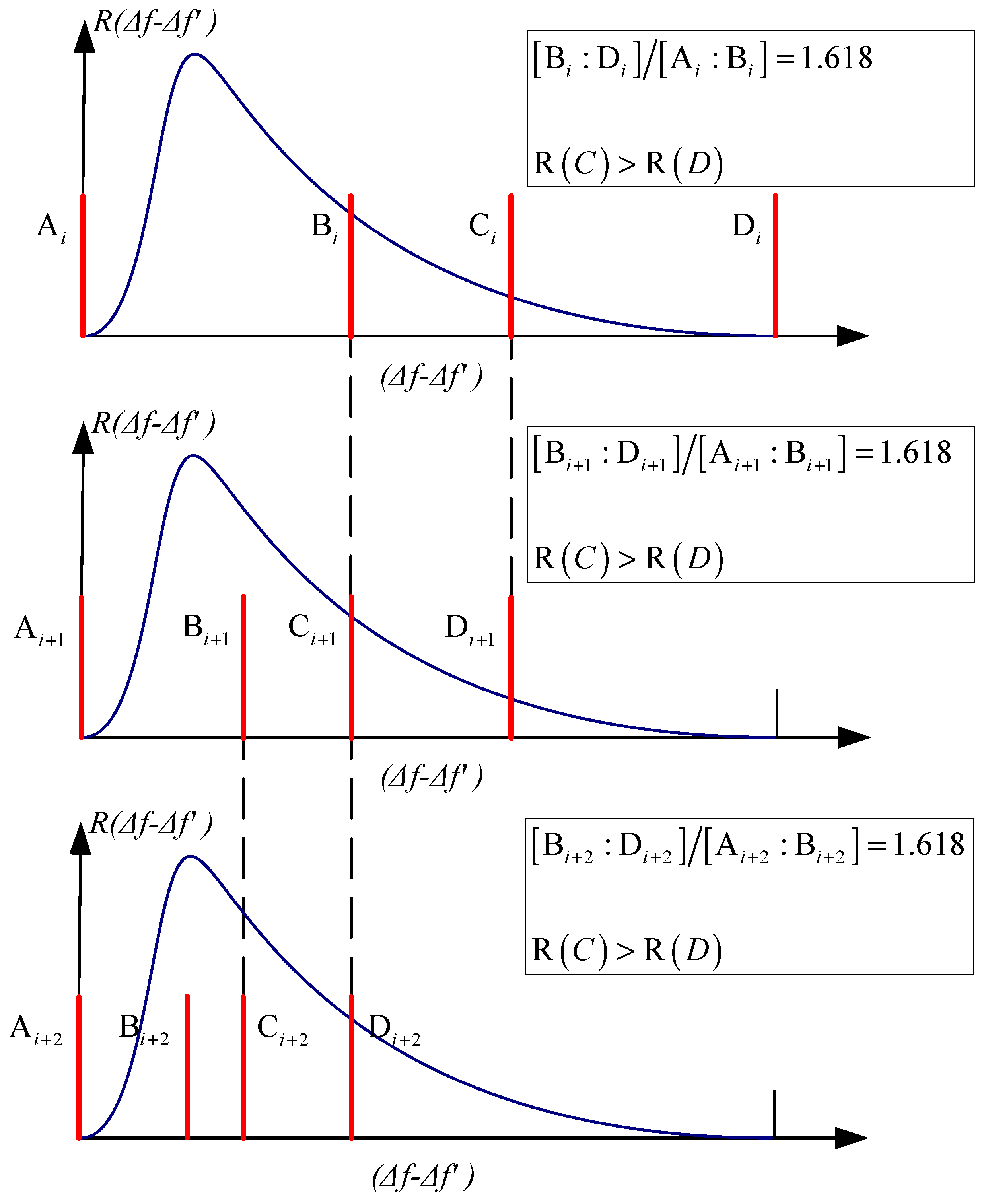
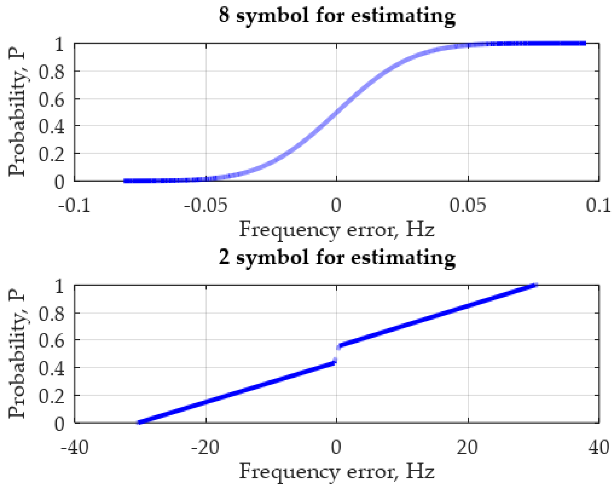
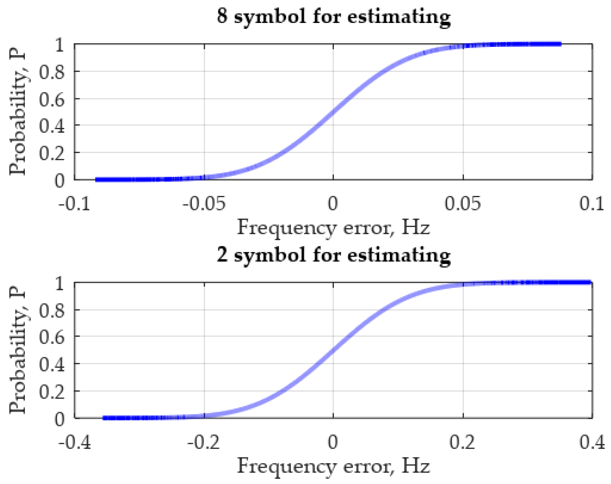
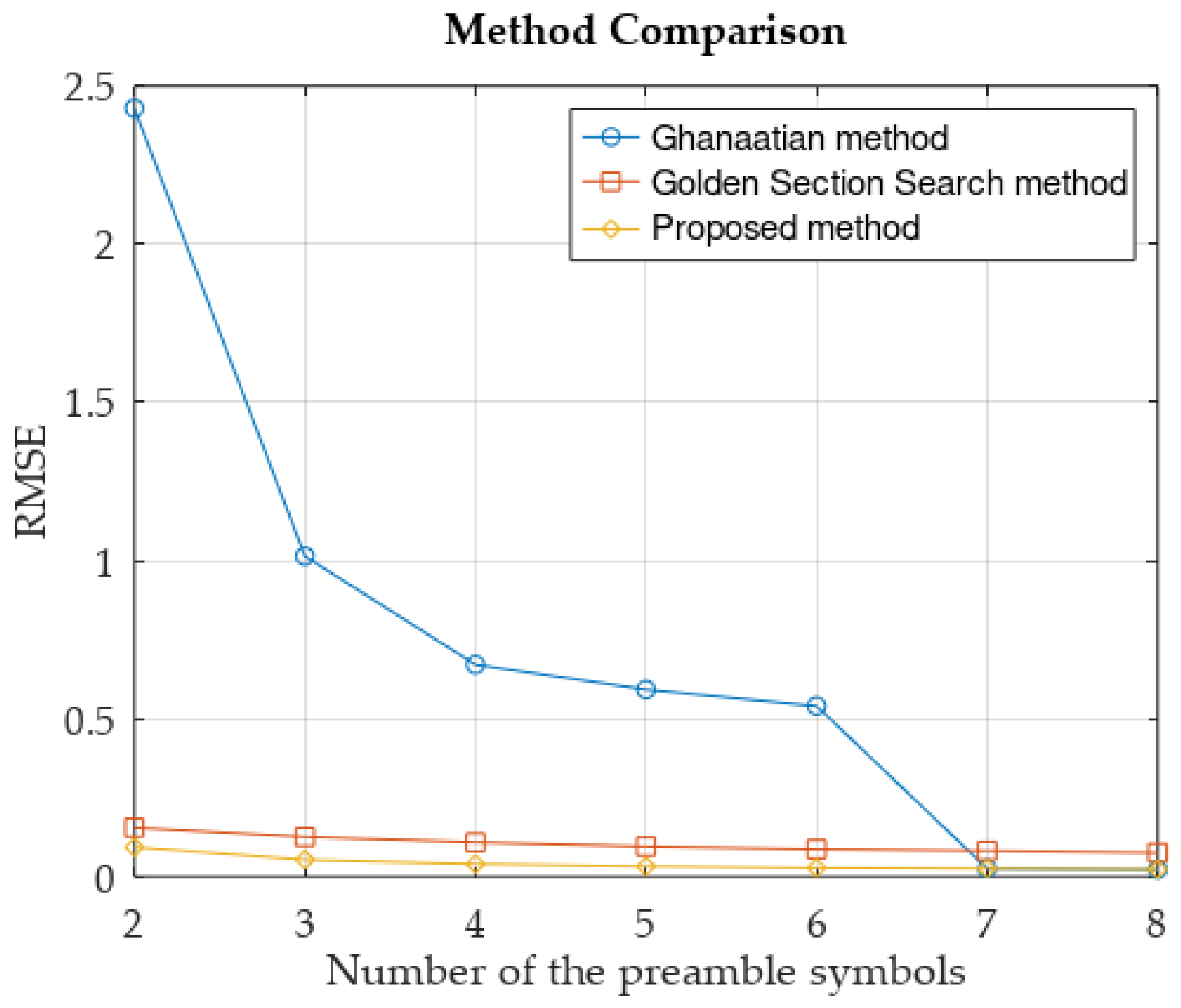
3. Results

In the model, the preamble symbols from 2 to 8 are used when performing the frequency estimation. Aside from frequency offset estimation and compensation, the CDF and RMSE of the frequency error estimation were calculated. Random frequency offset in the interval $\left[-3000:3000\right]$ Hz was used with the total number of iterations of 40,000.

Table 1. System parameters.

Parameter Name	Parameter Value
Signal bandwidth, $BW$	125 kHz
Sampling frequency, $f_{\mathrm{SR}}$	125 kHz
Spreading factor, $SF$	7
Signal-to-noise ratio, $SNR$	0 dB
Frequency estimation accuracy (GSS method)	1 Hz

shows the parameters of the model.

Based on [16], when using the chirp parameters given in Table 1, a bit error occurs when the frequency offset exceeds 488 Hz. Therefore, if there are cases when the frequency estimation error exceeds the value of 488 Hz, then it is concluded that the method works incorrectly.

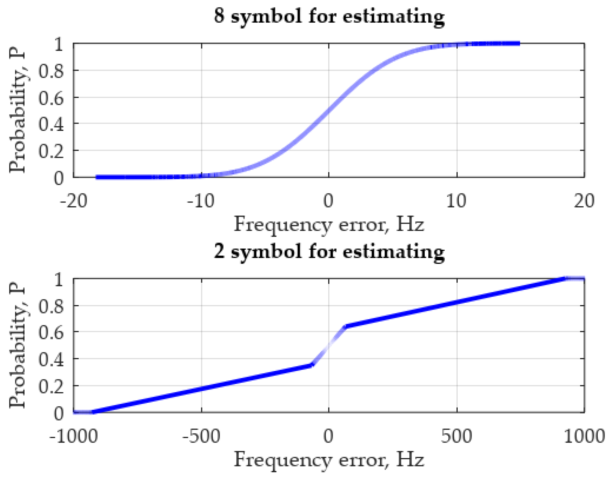
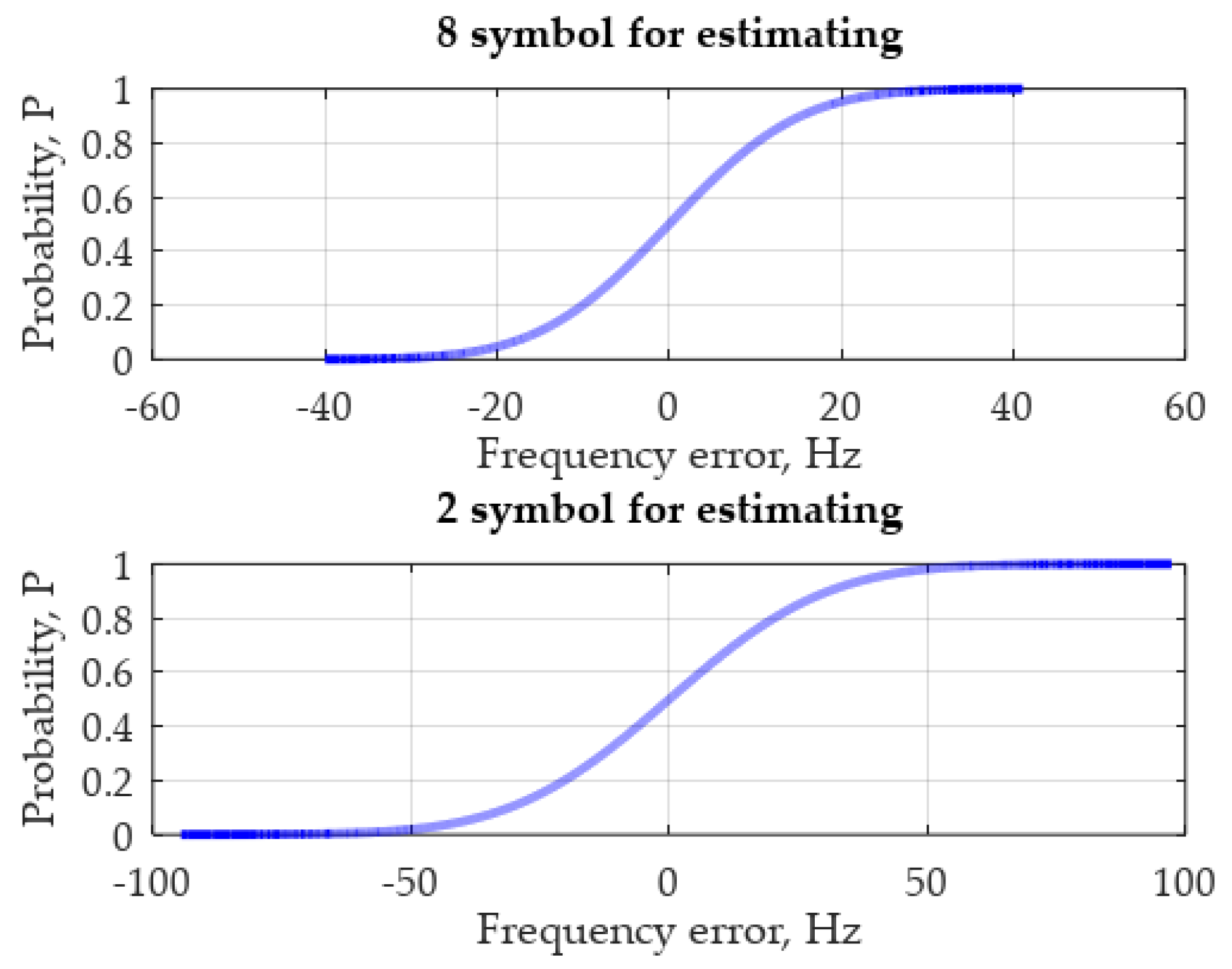
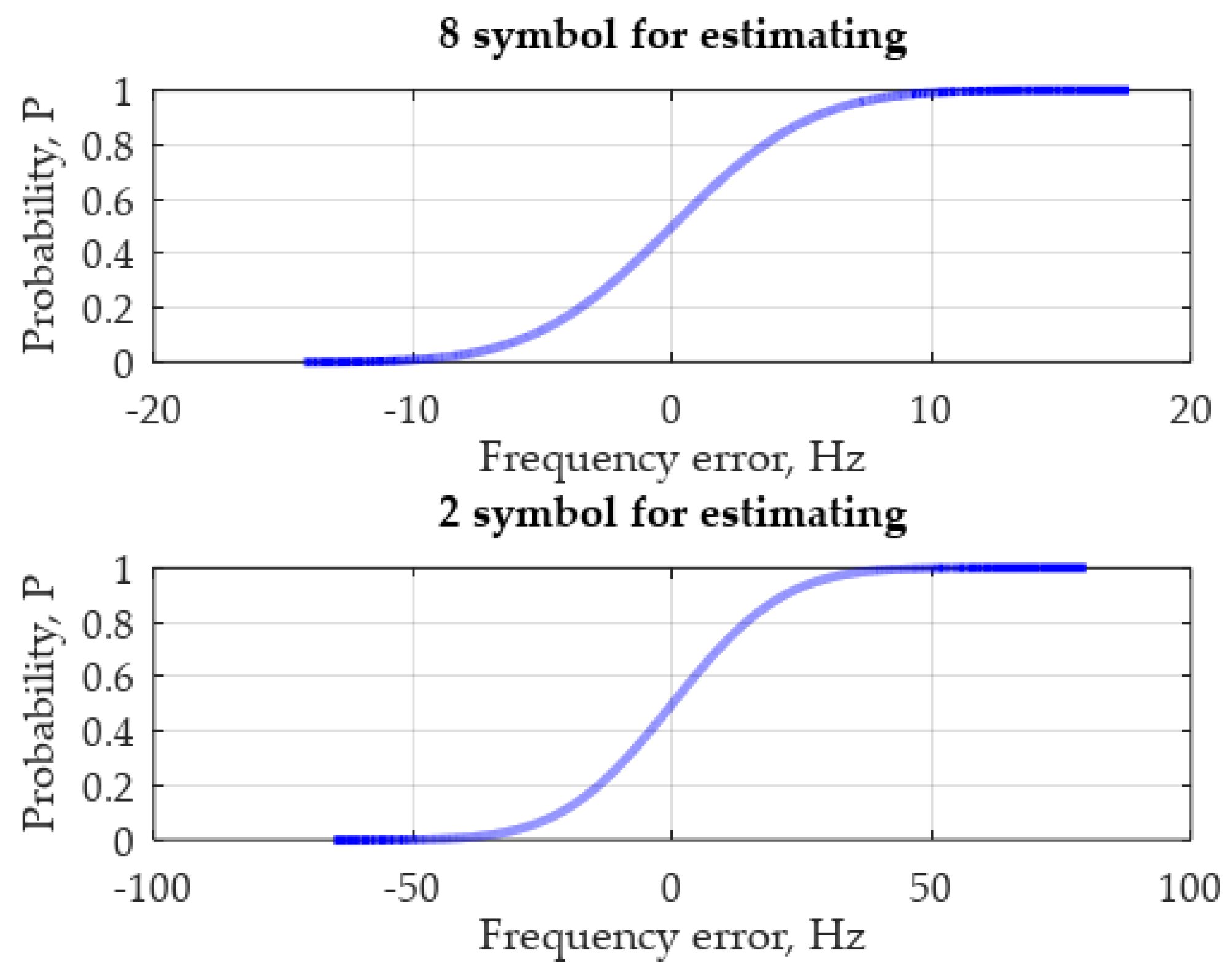
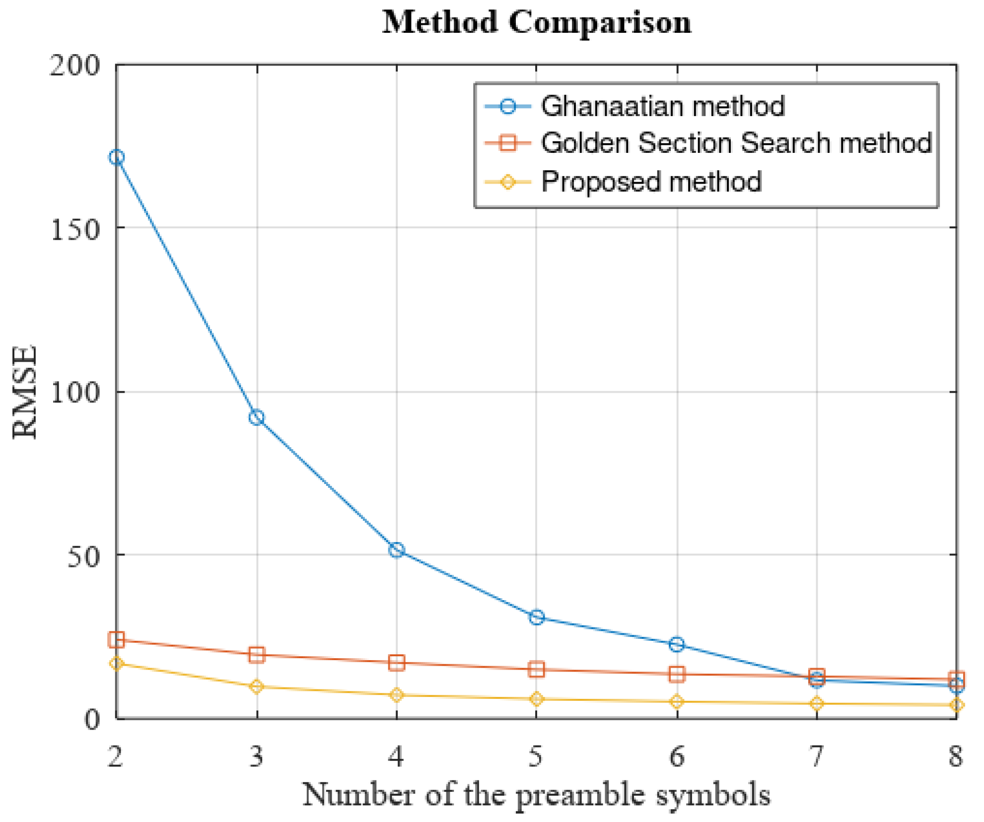
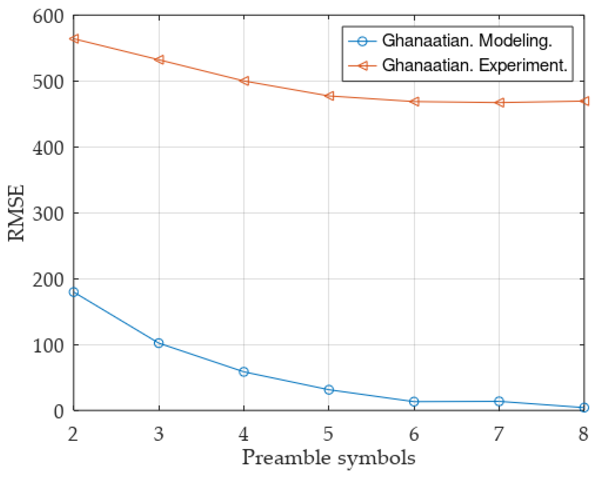
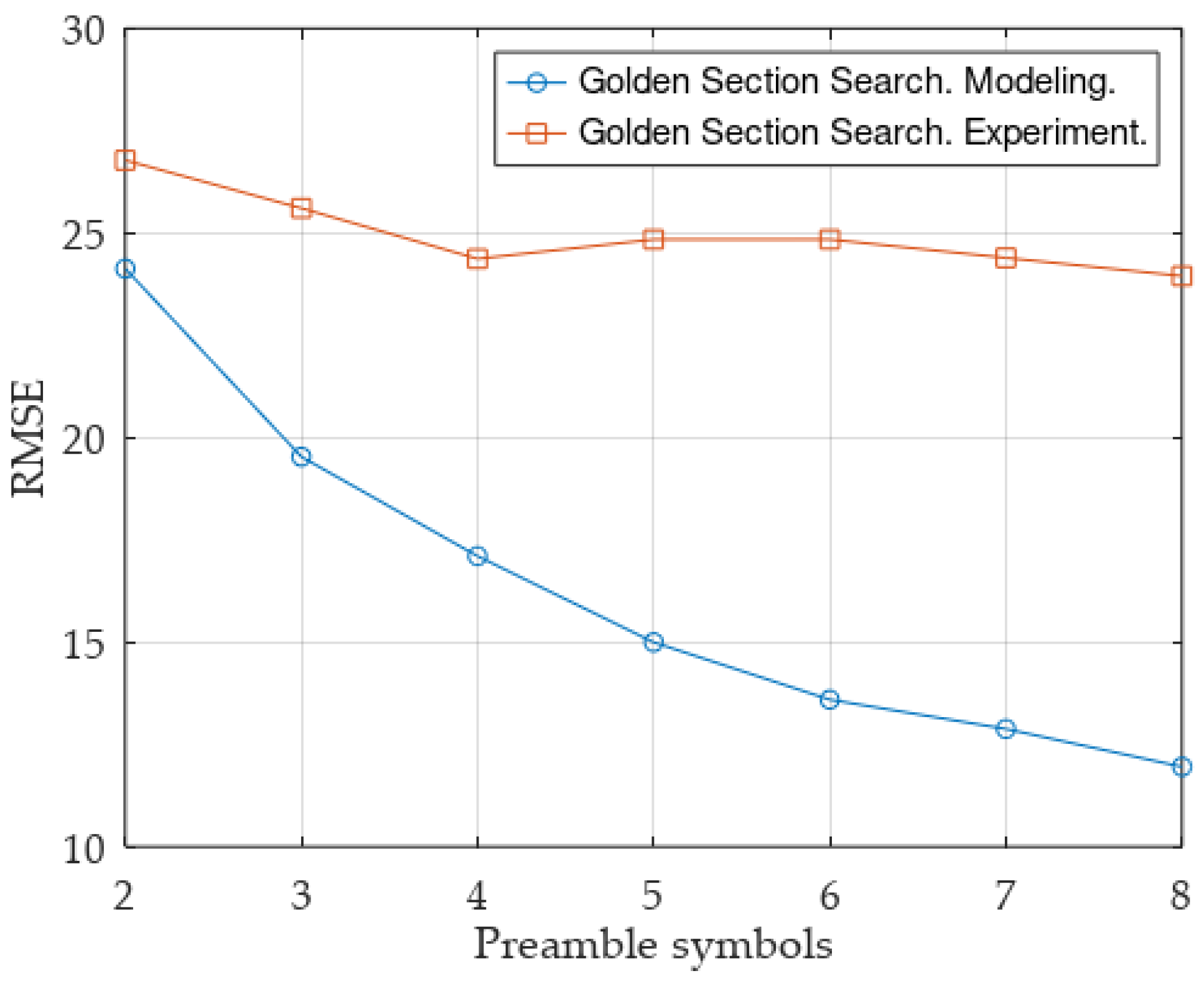
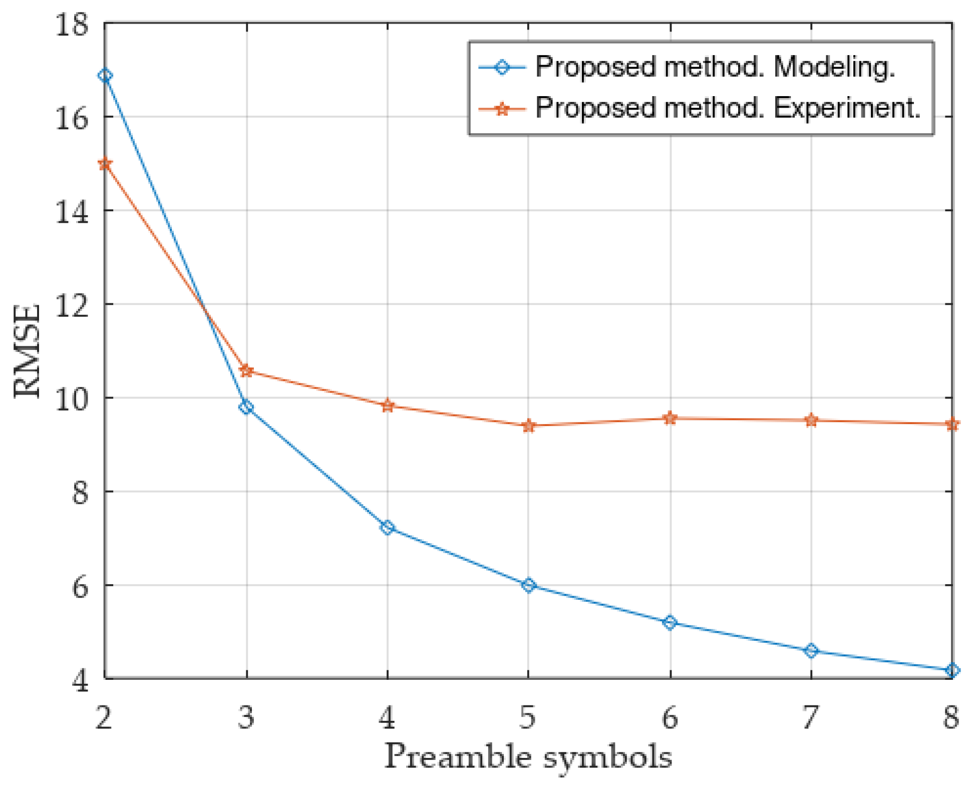
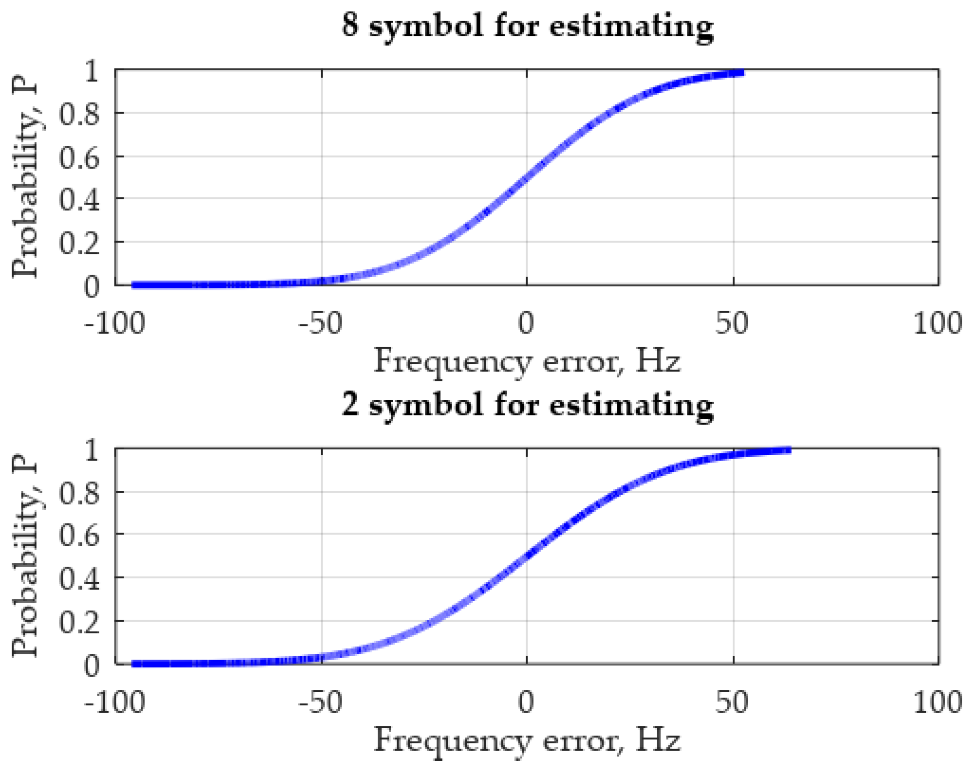
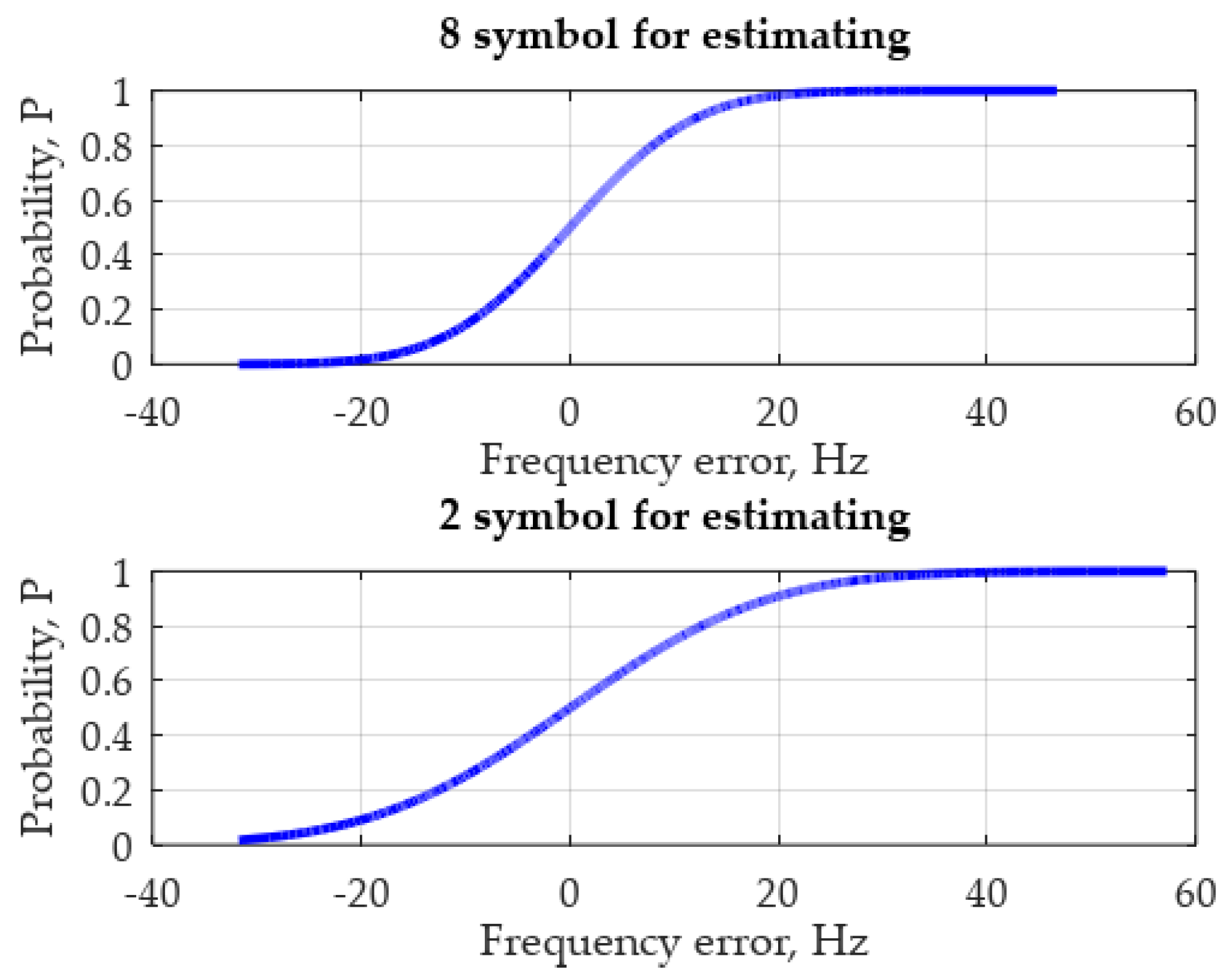
3.1. Discussion of Modeling Results

Figure 9, Figure 10 and Figure 11 show two cases: the CDF of the frequency estimation error when using two and eight preamble symbols with $SF=7$ to perform an estimation.

As can be seen from Figure 9, when using 2 preamble symbols, the Ghanaatian method worked incorrectly. In some cases, frequency error estimation was close in magnitude to the $f_{\mathrm{SAMP}}=976$ Hz (Figure 9).

As mentioned earlier, the frequency offset of this value is compensated with the use of a coarse estimation. Therefore, the problem is not coarse, but in an accurate frequency estimation. This is due to the sign ambiguity of the frequency estimation, as stated in Section 2.

Despite the fact that the frequency estimation accuracy GSS method was set equal to 1 Hz, from Figure 10, it can be seen that the frequency estimation error in some cases reached 100 Hz. Obviously, this error was due to a low SNR (0 dB).

The GSS method provides correct frequency offset estimation and compensation.

Figure 11 shows that the proposed method provided the most accurate frequency estimation compared to the two other methods.

After CDF calculation, the RMSE calculation is performed:

$$\mathrm{RMSE}=\sqrt{\frac{{\displaystyle \sum _{u=1}^M{\left(\delta f_u-\delta \overline{f}\right)}^2}}{M}}$$

(23)

where $u$ is an iteration number;

$M$ = 40,000 is the total amount of the iterations;

$\delta f_u$ is the frequency error estimation; and

$\delta \overline{f}$ is the average value of the vector frequency error estimation.

Figure 12 shows the dependence of the RMSE from the number of preamble symbols used. Below are the results provided by all methods.

As can be seen from Figure 12, when using up to six preamble symbols inclusive, the Ghanaatian method has the worst RMSE of all three methods. The RMSE in the GSS method is less than 82.5% at two symbols and 5.43% at six symbols. Furthermore, at seven and eight characters used, the Ghanaatian method worked slightly better than the GSS in 1% and 1.8%, respectively. The difference in the RMSE between these two methods was sharply reduced with an increase in the number of preamble symbols used. This was due to the presence of incorrect frequency estimations in the Ghanaatian method, which can be seen in Figure 9. Therefore, it can be concluded that this method is relevant when using a large number of preamble symbols. In other cases, the GSS is preferable due to the high frequency estimation accuracy. The proposed method provided the best RMSE less than 90% at two symbols and 2.9% at eight symbols compared with the Ghanaatian method, and less than 5.9% at two symbols and 4.6% at eight symbols compared with the GSS method. It can be seen that a sharp increase in the difference in the RMSE (the average value was 5.1%) with an increase in the number of symbols used did not occur.

Table 2. Comparison of the considered methods.

Characteristic	Ghanaatian	GSS	Proposed
Correctness of the estimation	Incorrect	Correct	Correct
Frequency estimation error	From 21 to 976 Hz	From 48 to 110 Hz	From 18 to 72 Hz
RMSE	From 10 to 171	From 13 to 25	From 5 to 18

shows the comparative analysis of the considered methods including the minimum and maximum values of the frequency correction error and the RMSE. Additionally, the correctness of the estimation is shown.

Based on the results obtained, it can be concluded that the proposed method showed the best results in frequency estimation accuracy. The GSS method was inferior to the accuracy, but allowed one to set the frequency estimation accuracy. The Ghanaatian method showed the worst results—the largest RMSE and the presence of incorrect frequency estimation.

For more information on the quality of the functioning of methods, modeling when $SF=12$ was performed. The CDF of the frequency estimation error when using two and eight preamble symbols is shown in Figure 13, Figure 14 and Figure 15. The dependence of the RMSE from the number of preamble symbols used is shown in Figure 16.

As can be seen from Figure 13, Figure 14, Figure 15 and Figure 16, when using $SF=12$, the accuracy of the frequency offset estimation provided by all methods increased significantly. The following key features can be noted:

• The Ghanaatian method provided the correct frequency offset estimation because according to [16], when the $SF=12$, demodulation errors occur if frequency error estimation exceeds 61 Hz
• The proposed method provided the most accurate frequency estimation.
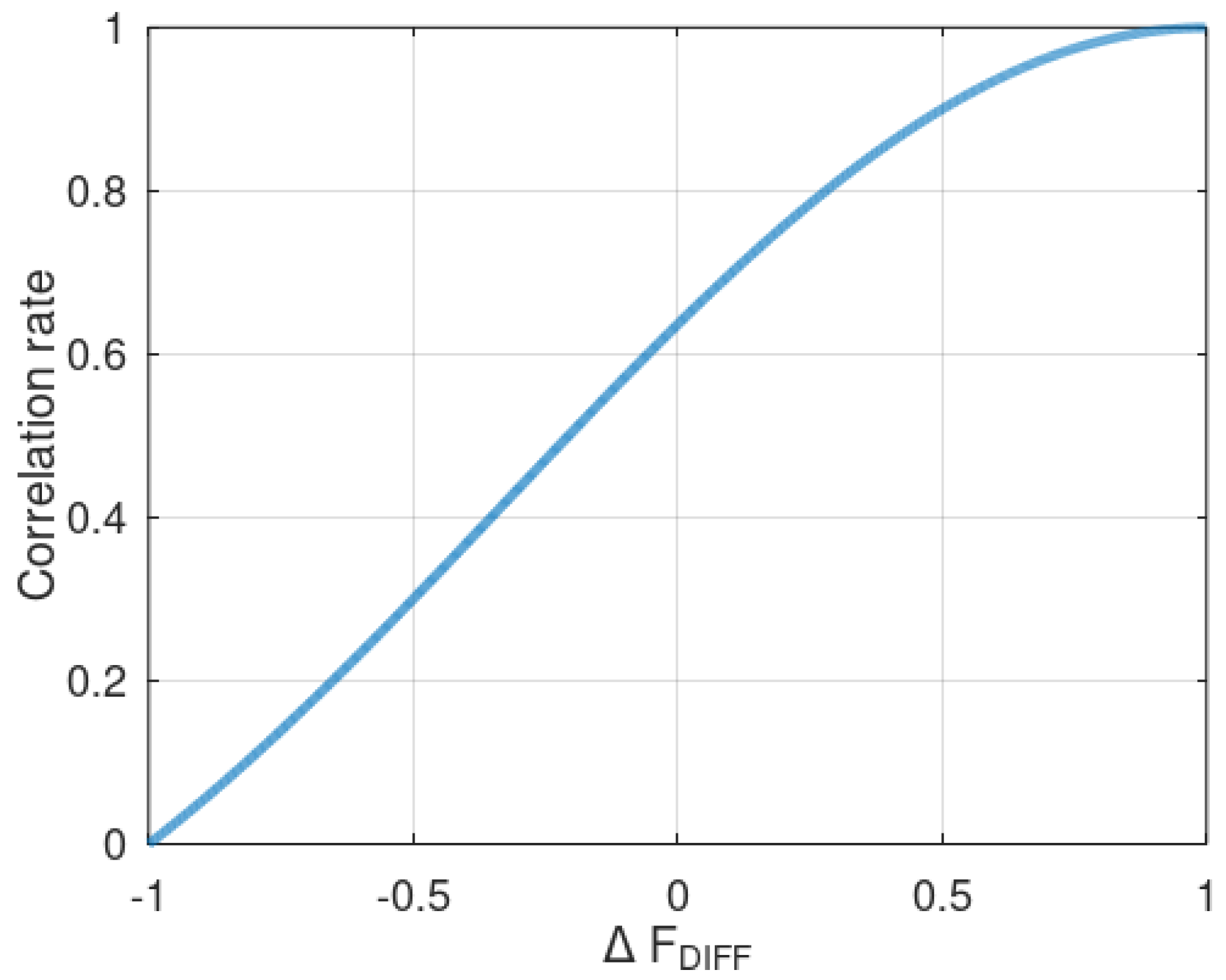
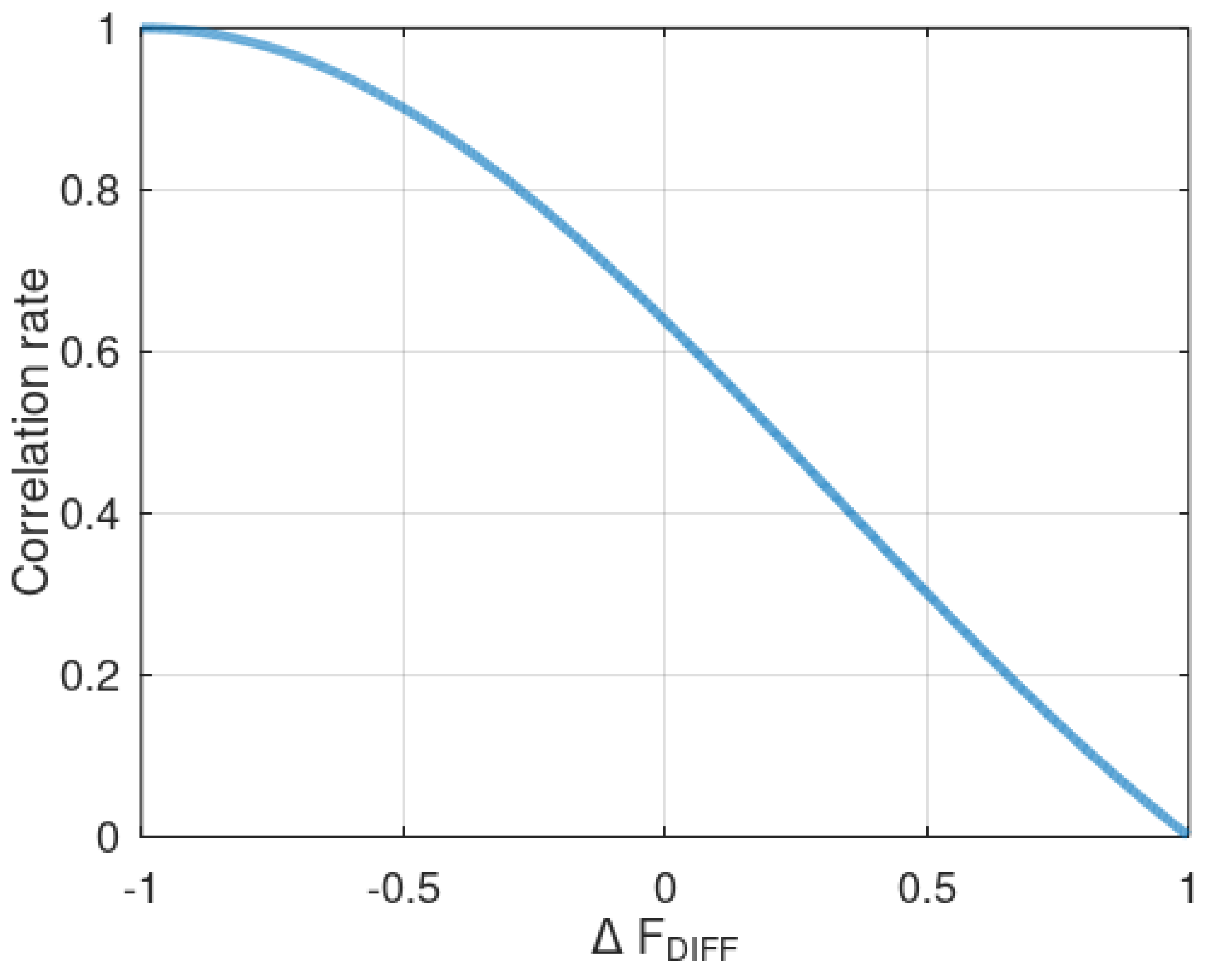
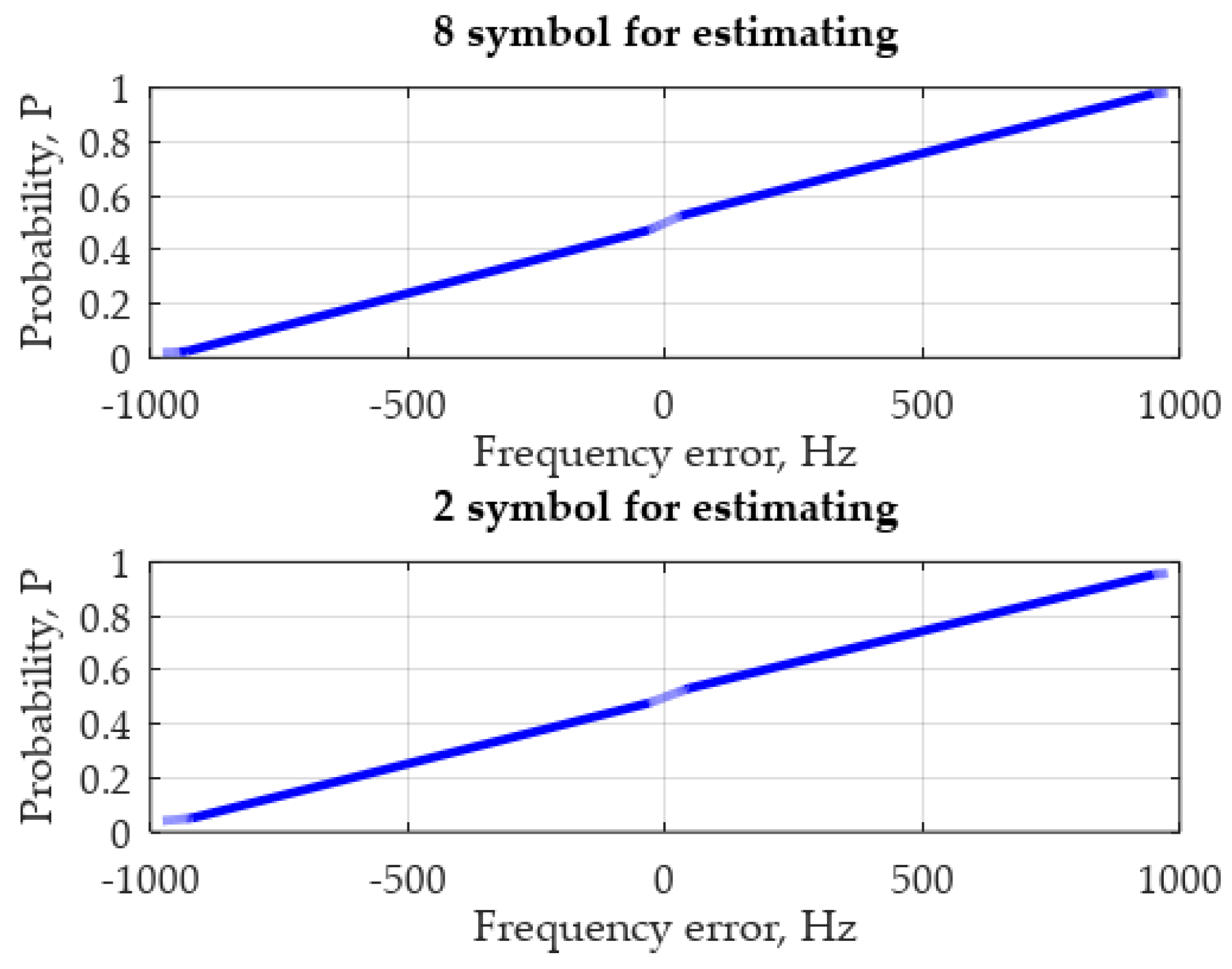
• Improving the frequency offset estimation can be explained by an increase in signal energy and these characteristics can deteriorate when SNR is low.

In addition, percentage ratio comparison of computational time considering methods was calculated. The Ghanaatian method computational time demonstrated the best result and was chosen as the reference time. Relative to the Ghanaatian method, the GGS method provided a computational time increase of up to 71% and the proposed method computational time increased up to 39%.

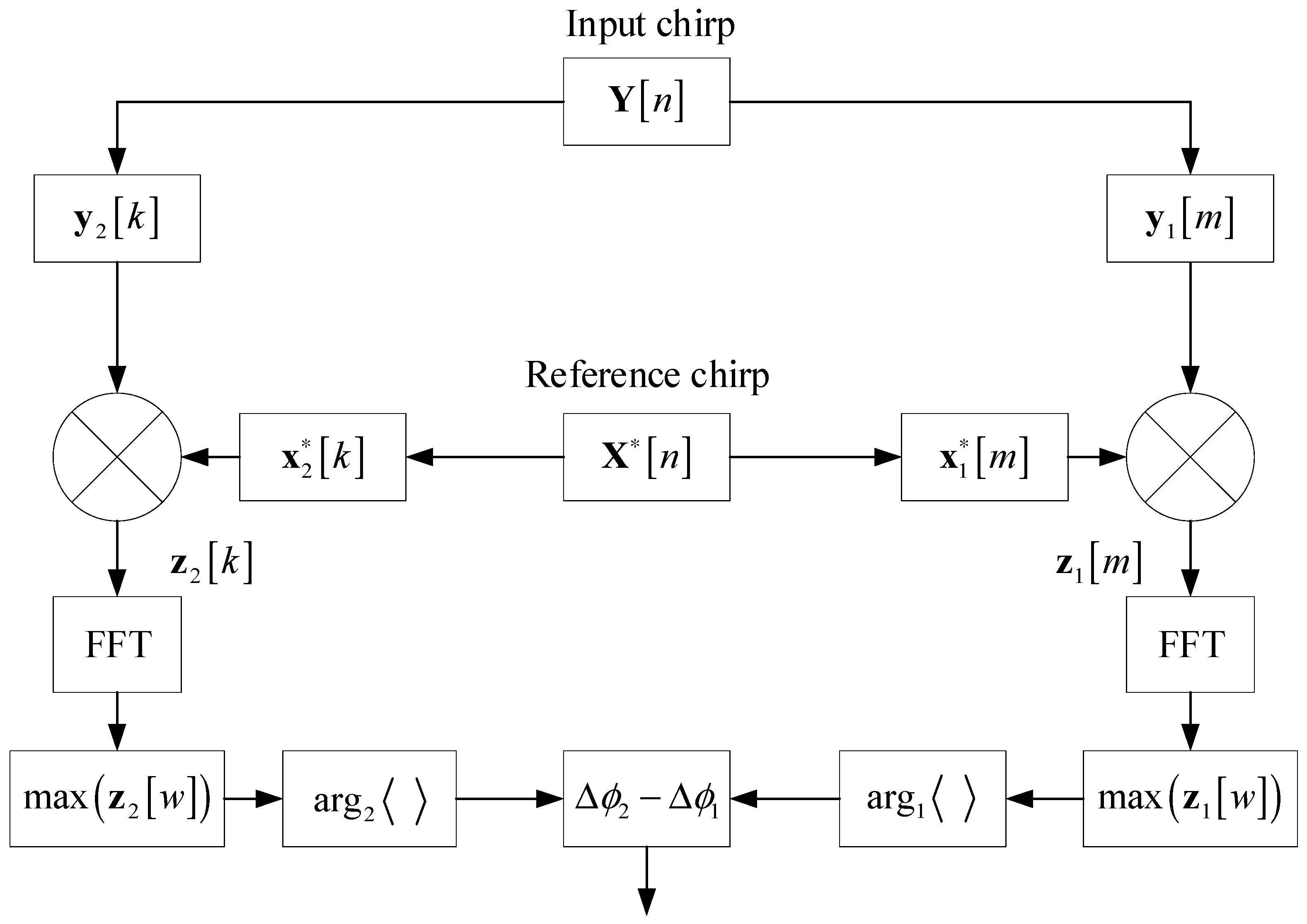
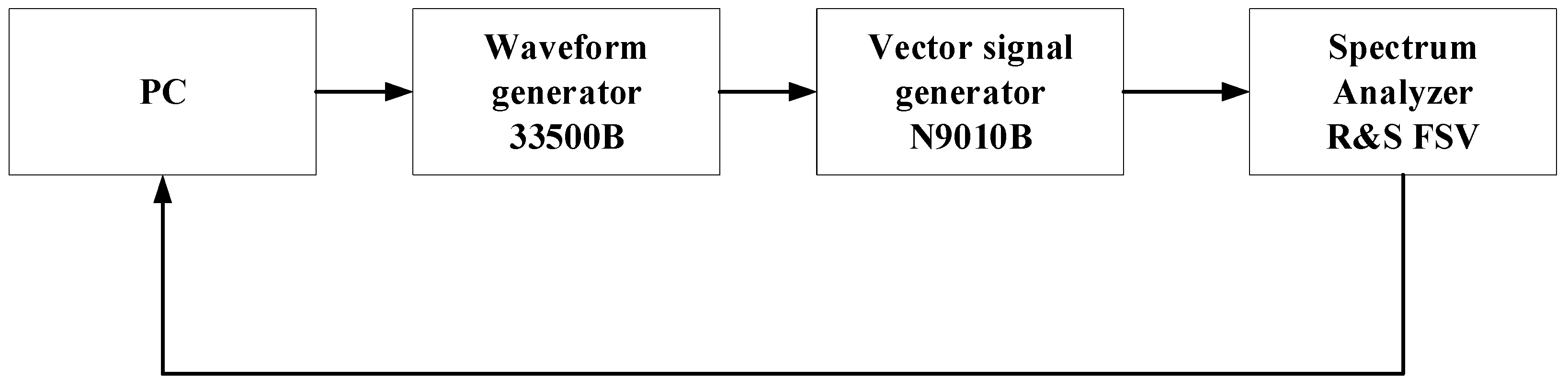
3.2. Experiment

The purpose of the study was to obtain results for the methods at the frequency offset equal to $f_{\mathrm{OFFSET}}=488$ Hz.

3.2.1. Program and Methods of Experimental Research

According to the scheme from Figure 17, an experimental stand was built.

The PC was used to create a massive of the chirp signals and send it to an arbitrary waveform generator model 33500B to perform digital to analog conversion. The N5166B vector signal generator was used to upconvert the signal to the frequency of 800 MHz. The ROHDE and SCHWARZ spectrum analyzer was used to receive the signal and upload the data to the PC. Then, the PC was used to process the received signals.

3.2.2. Discussion of Experiment Results

In the experiment, the value of the SNR was set to 0 dB. To receive data from spectrum analyzer, R&S IQWizard was used. Processing of the data on a PC was performed in GNU OCTAVE.

As a result of modeling, it was confirmed that the frequency offset of 488 Hz was the most critical for the considered configuration. For this reason, in the experiment, the frequency offset was set equal to 488 Hz using the vector signal generator N5166B.

3.2.3. Comparison Results of the Modeling and Experiment

Figure 18, Figure 19 and Figure 20 present the modeling comparison and experimental results. Figure 18 shows a comparison of the curves of the Ghanaatian method, Figure 19 shows the curves of the GSS method, and Figure 20 shows the curves of the proposed method, respectively.

To complete the calculation of the RMSE, for each method, we used the CDF calculation of the frequency error offset when using two and eight preamble symbols for averaging. The results are shown in Figure 21, Figure 22 and Figure 23.

4. Discussion

The divergence of results between the experiment and modeling results, especially the Ghanaatian algorithm was due to two factors:

• In the experiment, a non-coherent reception was performed (i.e., the phase of the signal was random); and
• Frequency offset was set to 488 Hz value. This is the most challenging case for frequency estimation methods.

The Ghanaatian method is sensitive to the frequency offset values defined in [16] and in low SNR conditions works incorrectly. The increase in the preamble characters used in performing the estimation significantly improved the estimation accuracy. The Ghanaatian method is not intended for use in low SNR conditions without performing additional estimation operations.

The GSS method provides the correct frequency estimation, and also allows the user to set the accuracy of the calculations. It also allows one to optimize the speed or the accuracy of the method. The significant drawbacks of the algorithm is the complexity of the calculations when using a high-precision estimation mode as well as a high influence of the SNR on the estimation results.

The proposed algorithm provides a more accurate frequency error estimation than the GSS and the Ghanaatian methods. The computational costs were close to the GSS method (when 1 Hz precision mode was used).

References

- Ghanaatian, R.; Afisiadis, O.; Cotting, M.; Burg, A. Lora Digital Receiver Analysis and Implementation. In Proceedings of the ICASSP 2019—2019 IEEE International Conference on Acoustics, Speech and Signal Processing (ICASSP), Brighton, UK, 12–17 May 2019; pp. 1498–1502. [Google Scholar] [CrossRef] [Green Version]
- Guan, P.; Yu, H.; Zhu, H.; Zhao, Y. A Novel Residual Carrier Frequency Offset Estimation Approach for LoRa Systems. In Proceedings of the 2020 5th International Conference on Computer and Communication Systems (ICCCS), Shanghai, China, 15–18 May 2020; pp. 830–834. [Google Scholar] [CrossRef]
- Raza, U.; Kulkarni, P.; Sooriyabandara, M. Low Power Wide Area Networks: An Overview. IEEE Commun. Surv. Tutor. 2017, 19, 855–873. [Google Scholar] [CrossRef] [Green Version]
- Mikhaylov, K.; Petajajarvi, J.; Hanninen, T. Analysis of capacity and scalability of the LoRa low power wide area network technology. In Proceedings of the European Wireless 2016, 22th European Wireless Conference, Oulu, Finland, 18–20 May 2016; pp. 1–6. [Google Scholar]
- Petajajarvi, J.; Mikhaylov, K.; Roivainen, A.; Hanninen, T.; Pettissalo, M. On the coverage of LPWANs: Range evaluation and channel attenuation model for LoRa technology. In Proceedings of the 14th International Conference on ITS Telecommunications (ITST), Copenhagen, Denmark, 2–4 December 2015; pp. 55–59. [Google Scholar] [CrossRef]
- Augustin, A.; Yi, J.; Clausen, T. A study of LoRa: Long range & low power networks for the Internet of Things. Sensors 2016, 16, 1466. [Google Scholar] [CrossRef]
- Nolan, K.E.; Guibene, W.; Kelly, M.Y. An evaluation of low power wide area network technologies for the Internet of Things. In Proceedings of the 2016 International Wireless Communications and Mobile Computing Conference (IWCMC), Paphos, Cyprus, 5–9 September 2016; pp. 439–444. [Google Scholar] [CrossRef]
- Sornin, N.; Bertolaud, A.; Delclef, J.; Delport, V.; Duffy, P.; Dyduch, F.; Eirich, T.; Ferreira, L.; Gharout, S.; Hersent, O.; et al. LoRaWAN Specification; LoRa Alliance: Fremont, CA, USA, 2016. [Google Scholar]
- Kim, B.; Hwang, K. Cooperative Downlink Listening for Low-Power Long-Range Wide-Area Network. Sustainability 2017, 9, 627. [Google Scholar] [CrossRef] [Green Version]
- Conus, G.; Lilis, G.; Zanjani, N.A.; Kayal, M. An event-driven low power electronics for loads metering and control in smart buildings. In Proceedings of the 2016 Second International Conference on Event-Based Control, Communication, and Signal Processing (EBCCSP), Krakow, Poland, 13–15 June 2016; pp. 1–7. [Google Scholar] [CrossRef]
- Sartori, D.; Brunelli, D. A smart sensor for precision agriculture powered by microbial fuel cells. In Proceedings of the IEEE Sensors Applications Symposium (SAS), Catania, Italy, 20–22 April 2016; pp. 1–6. [Google Scholar] [CrossRef]
- Chen, L.-Y.; Huang, H.-S.; Wu, C.-J.; Tsai, Y.-T.; Chang, Y.-S. A LoRa-Based Air Quality Monitor on Unmanned Aerial Vehicle for Smart City. In Proceedings of the 2018 International Conference on System Science and Engineering (ICSSE), New Taipei, Taiwan, 28–30 June 2018; pp. 1–5. [Google Scholar] [CrossRef]
- Robson, S.; Haddad, A.M. On the use of LoRa for power line communication. In Proceedings of the 54th International Universities Power Engineering Conference (UPEC), Bucharest, Romania, 3–6 September 2019; pp. 1–6. [Google Scholar] [CrossRef]
- Fernandez, L.; Ruiz-De-Azua, J.A.; Calveras, A.; Camps, A. Assessing LoRa for Satellite-to-Earth Communications Considering the Impact of Ionospheric Scintillation. IEEE Access 2020, 8, 165570–165582. [Google Scholar] [CrossRef]
- Qian, Y.; Ma, L.; Liang, X. Symmetry chirp spread spectrum modulation used in LEO satellite Internet of Things. IEEE Commun. Lett. 2018, 22, 2230–2233. [Google Scholar] [CrossRef]
- Mukhamadiev, S.M.; Dmitriyev, E.M.; Rogozhnikov, E.V.; Duplishcheva, N.V.; Kryukov, Y.V. The Effect of Frequency Offset on the Probability of Bit and Packet Errors in Processing Signals with Chirp Spread Spectrum Modulation. In Proceedings of the 2021 International Siberian Conference on Control and Communications (SIBCON), Kazan, Russia, 13–15 May 2021; pp. 1–5. [Google Scholar] [CrossRef]
- Bohlin, T. On the maximum likelihood method of identification. IBM J. Res. Dev. 1970, 14, 41–51. [Google Scholar] [CrossRef]
- A Technical Overview of LoRa® and LoRaWAN®. Available online: https://lora-alliance.org/wp-content/uploads/2020/11/what-is-lorawan.CDF (accessed on 9 March 2022).
- Liando, J.C.; Gamage, A.; Tengourtius, A.W.; Li, M. Known and Unknown Facts of LoRa: Experiences from a large-scale measurement study. ACM Trans. Sens. Netw. 2019, 15, 1–35. [Google Scholar] [CrossRef]
- RP002-1.0.3 LoRaWAN® Regional Parameters. Available online: https://lora-alliance.org/wp-content/uploads/2021/05/RP002-1.0.3-FINAL-1.CDF (accessed on 9 March 2022).
- Vangelista, L. Frequency shift chirp modulation: The LoRa modulation. IEEE Signal Process. Lett. 2017, 24, 1818–1821. [Google Scholar] [CrossRef]
- Al Homssi, B.; Dakic, K.; Maselli, S.; Wolf, H.; Kandeepan, S.; Al-Hourani, A. IoT Network Design Using Open-Source LoRa Coverage Emulator. IEEE Access 2021, 9, 53636–53646. [Google Scholar] [CrossRef]
- Chiani, M.; Elzanaty, A. On the LoRa modulation for IoT: Waveform properties and spectral analysis. IEEE Internet Things J. 2019, 6, 8463–8470. [Google Scholar] [CrossRef] [Green Version]
- Elshabrawy, T.; Robert, J. Closed-form approximation of LoRa modulation BER performance. IEEE Commun. Lett. 2018, 22, 1778–1781. [Google Scholar] [CrossRef]
- Fletcher, R. Practical Methods of Optimization; John Wiley & Sons: Hoboken, NJ, USA, 1980. [Google Scholar]
- Four-Quadrant Inverse Tangent Documentation. Available online: https://www.mathworks.com/help/matlab/ref/atan2d.html#b-u4zyzh (accessed on 9 March 2022).
- Angrisani, L.; Arpaia, P.; Bonavolonta, F.; Conti, M.; Liccardo, A. LoRa protocol performance assessment in critical noise conditions. In Proceedings of the 2017 IEEE 3rd International Forum on Research and Technologies for Society and Industry (RTSI), Modena, Italy, 11–13 September 2017; pp. 1–5. [Google Scholar] [CrossRef]