Article

Mathematical Modeling and Analysis of Tumor Chemotherapy

1
Department of Information and Computational Science, Henan Agricultural University, Zhengzhou 450002, China
2
School of Mathematics and Statistics, Central China Normal University, Wuhan 430079, China
3
School of Mathematics and Statistics, Xinxiang University, Xinxiang 453000, China
4
School of Mathematics, Monash University, Melbourne, VIC 3800, Australia
*
Authors to whom correspondence should be addressed.
Symmetry 2022, 14(4), 704; https://doi.org/10.3390/sym14040704
Submission received: 7 March 2022 / Revised: 25 March 2022 / Accepted: 25 March 2022 / Published: 31 March 2022
(This article belongs to the Special Issue Symmetries in Differential Equation and Application)

Abstract

:
Cancer diseases lead to the second-highest death rate all over the world. For treating tumors, one of the most common schemes is chemotherapy, which can decrease the tumor size and control the progression of cancer diseases. To better understand the mechanisms of chemotherapy, we developed a mathematical model of tumor growth under chemotherapy. This model includes both immune system response and drug therapy. We characterize the symmetrical properties and dynamics of this differential equation model by finding the equilibrium points and exploring the stability and symmetry properties in a range of model parameters. Sensitivity analyses suggest that the chemotherapy drug-induced tumor mortality rate and the drug decay rate contribute significantly to the determination of treatment outcomes. Numerical simulations highlight the importance of CTL activation in tumor chemotherapy.

1. Introduction

The tumor is a complex disease, which is the second leading cause of death in the world [1,2]. The death rate caused by cancer has been increased worldwide in recent years [3]. Although substantial medical research studies have been conducted, more research studies are strongly needed to understand the mechanism of cancer initiation and destruction as well as the effects of the anti-tumor therapy. Mathematical models provide a valuable theoretical framework through which immuno-oncological mechanisms can be discovered and clarified [4,5,6,7,8]. The applications of mathematical models enable us to study the dynamics and symmetrical property of the immune system as well as to discover the mechanisms controlling tumor cells, to design the therapy schemes, and to predict the outcomes of new therapy strategies [9,10,11,12,13,14,15,16,17,18,19]. In addition, theoretical analysis, modeling methodologies, and symmetrical analysis techniques have been applied to investigate various properties of mathematical models using differential equations [20,21,22,23].
Medical practices show that surgery, chemotherapy, immunotherapy, and radiation therapy so far are the widely used clinical schemes to treat cancer diseases successfully [11,12,13,14,15,16,17,18]. However, the treatment outcome depends on a number of factors, including the type and degree of the tumor, the implementation of treatment schemes, and the intensity of the patient’s autoimmune response. Mathematical modeling provides a theoretical framework to predict the long-term treatment outcomes, which is difficult to be realized by clinical studies. Currently, there are a variety of mathematical models for tumor growth and treatment. However, each model only studies a couple of important factors in cancer diseases and the medical treatment effects [14,15,16,17,18,24,25,26,27,28,29,30,31,32].
Among the treatment schemes for tumor diseases, the most common one is chemotherapy. In the work of A.G. López et al. [11], they proposed a dynamical model of tumor growth, which includes the interactions and regulations between tumor cells, healthy host cells, and immune effector cells. By analyzing the dynamical properties of the model, they demonstrated the consistency between the theoretical analysis and empirical discovery regarding the tumor progression and immune function. They introduced a chemotherapeutic treatment scheme and proposed an approach to overcome problems in complex pharmacokinetic modeling. A follow-up study proposed a differential equations model for the interactions of tumor cells and immune cells under chemotherapy [13]. This study suggested that intense chemotherapies could result in inferior tumor control. In addition, more intense therapies might result in a stronger depletion of immune cells, which allows an early re-growth of the tumor. However, these studies neither accounted for the different cell populations of innate and specific immune responses nor contained complex pharmacokinetics.
Motivated by the need to better understand the mechanisms of chemotherapy treatment and find more efficacious therapeutic methods, we propose a mathematical model to study the effects of the immune system and chemotherapy to treat cancer diseases. The purpose of this study is to explore the combined beneficial effects of the immune system to regulate tumor growth and to find the side effects of chemotherapeutic drugs on both the tumor cells and effector cells. Compared to previous models, the main innovation of this work is the combination of important functions of the immune system and the representation of dose-response dynamics in terms of mass action rather than exponential decay. Thus, the proposed model describes three types of cells and one drug concentration. We first analyze the local geometric and symmetrical properties of the equilibria of the proposed model and then use simulations to confirm the theoretical results. In addition, sensitivity analysis finds important parameters that have more impact on the variations of tumor cell numbers, which provide predictions for designing treatment schemes.

2. The Model

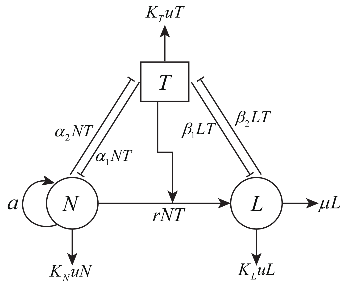
2.1. Mathematical Model

We first propose a mathematical model to describe the interaction of tumor cells and the anti-tumor immune system, as well as the influence of chemotherapy on both tumor cells and the immune system. The model variables are T ( t ) for tumor cell population at time t, N ( t ) for NK cell population, L ( t ) for cytotoxic T cell (CTLs) population, and u ( t ) for the amount of drug at the tumor site. Figure 1 gives the schematic diagram for the interactions of these variables. The proposed model is based on the following assumptions.
  • Both immune effector cells and chemotherapy decrease the tumor population.
  • The population of effector cells decreases due to the degradation process, consumption when killing tumor cells, and the effect of chemotherapy.
  • Chemotherapy drugs can affect tumor cells and immune effector cells through a mass-action mechanism.
  • A higher constant input of the drug dose can result in both higher tumor and immune effector cell depletion.
The proposed model describes the population dynamics of tumor cells and the immune system under chemotherapy, given by
N ( t ) = a N ( t ) ( 1 b N ( t ) ) α 1 N ( t ) T ( t ) k N u ( t ) N ( t ) , L ( t ) = r N ( t ) T ( t ) μ L ( t ) β 1 L ( t ) T ( t ) k L u ( t ) L ( t ) , T ( t ) = c T ( t ) ( 1 d T ( t ) ) α 2 N ( t ) T ( t ) β 2 L ( t ) T ( t ) k T u ( t ) T ( t ) , u ( t ) = v ω u ( t ) ,
with initial conditions N ( 0 ) = N 0 0 , L ( 0 ) = L 0 0 , T ( 0 ) = T 0 0 , and u ( 0 ) = u 0 0 .
In the first equation of model (1), it is assumed that NK cells grow logistically through the term a N ( t ) ( 1 b N ( t ) ) . However, they are inactivated through the interactions with tumor cells based on α 1 N ( t ) T ( t ) . In the second equation, CTLs are present in the system when the tumor cells are present. They are recruited by tumor cells through a linear term r N ( t ) T ( t ) . In addition, the death of CTLs is a linear process μ L ( t ) . In addition, the interactions with tumor cells will inactivate CTLs via β 1 L ( t ) T ( t ) . In the third equation, tumor is assumed to grow according to a logistic function as c T ( t ) ( 1 d T ( t ) ) [12,13,14,18,24,25]. In addition, the tumor cells are killed by both NK cells and CTLs, which are realized by α 2 N ( t ) T ( t ) and β 2 L ( t ) T ( t ) , respectively. The chemotherapy drug in the last equation has a constant source v, and linearly fades out of the system by ω u ( t ) . In our model (1), since the chemotherapy drug affects all three cell populations through a mass-action dynamic and the drug mortality rate differs for each type of cell, we denote the three different response coefficients by k N , k L , and k T . Table 1 lists the parameters in model (1), along with their units, descriptions, estimated values, and references.

2.2. The Reduced Model

To reduce the model complexity, we use the following non-dimensionalized state variables to simplify the model, given by
N ¯ = α 2 μ N , L ¯ = α 1 α 2 r μ L , T ¯ = α 1 μ T , u ¯ = k N μ , d t = 1 μ d τ .
Then the simplified model is
N ¯ ( τ ) = a μ N ¯ ( τ ) ( 1 b μ α 2 N ¯ ( τ ) ) N ¯ ( τ ) T ¯ ( τ ) u ¯ ( τ ) N ¯ ( τ ) , L ¯ ( τ ) = N ¯ ( τ ) T ¯ ( τ ) L ¯ ( τ ) β 1 α 1 L ¯ ( τ ) T ¯ ( τ ) u ¯ ( τ ) L ¯ ( τ ) , T ¯ ( τ ) = c μ T ¯ ( τ ) ( 1 d μ α 1 T ¯ ( τ ) ) N ¯ ( τ ) T ¯ ( τ ) r β 2 α 1 α 2 L ¯ ( τ ) T ¯ ( τ ) k T k N u ¯ ( τ ) T ¯ ( τ ) , u ¯ ( τ ) = k N v μ 2 ω μ u ¯ ( τ ) .
By rewriting N ¯ , L ¯ , T ¯ , u ¯ , τ as N , L , T , u , and t, respectively, we have the following dimensionless model, given by
N ( t ) = p N ( t ) ( 1 1.8 × 10 2 N ( t ) ) N ( t ) T ( t ) u ( t ) N ( t ) , L ( t ) = N ( t ) T ( t ) L ( t ) 3.42 × 10 3 L ( t ) T ( t ) u ( t ) L ( t ) , T ( t ) = 25.7 T ( t ) ( 1 2.04 × 10 4 T ( t ) ) N ( t ) T ( t ) 6.02 × 10 3 L ( t ) T ( t ) k u ( t ) T ( t ) , u ( t ) = s f u ( t ) ,
where p = a μ , k = k T k N , s = k N v μ 2 , f = ω μ . Using the values in Table 1, the values in model (3) are b μ α 2 = 1.8 × 10 2 , β 1 α 1 = 3.42 × 10 3 , c μ = 2.57 × 10 , d μ α 1 = 2.04 × 10 4 , and r β 2 α 1 α 2 = 6.02 × 10 3 .

3. Dynamics

This section will first find the positive invariant set of model (3). Then we study the existence of equilibrium states and their corresponding stability properties. We give the first result for the positive invariant set.
Lemma 1.
The solutions of model (3) are positive if all initial values are positive and R + 4 = { ( N ( t ) , L ( t ) , T ( t ) , u ( t ) ) | N ( t ) 0 , L ( t ) 0 , T ( t ) 0 , u ( t ) 0 } is a positive invariant set of model (3).
Proof. 
Let X ( t ) = ( N ( t ) , L ( t ) , T ( t ) , u ( t ) ) be a positive solution of model (3) based on the initial solution X ( 0 ) = ( N 0 , L 0 , T 0 , u 0 ) R + 4 . Following the dimensionless model (3), we have the following equations
N ( t ) = N 0 e 0 t ( p ( 1 1.8 × 10 2 N ( m ) ) T ( m ) u ( m ) ) d m , L ( t ) L ( t ) 3.42 × 10 3 L ( t ) T ( t ) u ( t ) L ( t ) , T ( t ) = T 0 e 0 t ( 2.57 × 10 ( 1 2.04 × 10 4 T ( m ) ) N ( m ) 6.02 × 10 3 L ( m ) k u ( m ) ) d m , u ( t ) = u 0 e 0 t ( s u ( m ) f ) d m .
If N 0 0 , T 0 0 , and u 0 0 , we can derive that N ( t ) 0 , T ( t ) 0 , u ( t ) 0 . In addition, the second inequality in (4) gives
L ( t ) L 0 e 0 t ( 1 3.42 × 10 3 T ( m ) u ( m ) ) d m .
Using the comparison principle, we can obtain that, if L 0 0 , then L ( t ) 0 . Thus, if N 0 0 , , T 0 0 , u 0 0 , then N ( t ) 0 , L ( t ) 0 , T ( t ) 0 , u ( t ) 0 . That is, all solutions of model (3) are positive when their initial values are positive. Thus, R + 4 is a positively invariant set of model (3). □

3.1. Equilibria of Dimensionless Model

We first note that the fourth equation in (3) can be decoupled from the model. The equilibrium of variable u is u = s f . Thus, we need to consider the model with the remaining three equations,
N ( t ) = p N ( t ) ( 1 1.8 × 10 2 N ( t ) ) N ( t ) T ( t ) u ( t ) N ( t ) L ( t ) = N ( t ) T ( t ) L ( t ) 3.42 × 10 3 L ( t ) T ( t ) u ( t ) L ( t ) T ( t ) = 25.7 T ( t ) ( 1 2.04 × 10 4 T ( t ) ) N ( t ) T ( t ) 6.02 × 10 3 L ( t ) T ( t ) k u ( t ) T ( t ) .
We set each equation equals to zero. The null-surfaces of model (6) are given by
N ( t ) = 0 N = 0 o r N = p T u 1.8 × 10 2 p , L ( t ) = 0 L = ( p T u ) T 1.8 × 10 2 p ( 1 + 3.42 × 10 3 T + u ) , T ( t ) = 0 T = 0 o r T = 1.91 × 10 2 ( 25.7 N 6.02 × 10 3 L k u ) .
where u = s f . Then the types of equilibrium states can be given as follows.
(i) The dead state, at which all three cell populations are zero, namely
E 0 ( 0 , 0 , 0 , s f )
(ii) The tumor-free state, at which the population of tumor cells is zero but the NK cells survive. The equilibrium point is given by
E 1 ( p s f 1.8 × 10 2 p , 0 , 0 , s f ) , w h e n p > s f .
(iii) The tumor-present state, at which the populations of NK cells and CTLs are zero but the tumor cells survive.
E 2 ( 0 , 0 , 1.91 × 10 2 ( 25.7 k s f ) , s f ) , w h e n 25.7 > k s f .
(iv) The coexisting state, at which immune and tumor cells have nonzero populations. There are the following possible equilibrium states E 3 ( N i , L i , T i , s f ) , ( i = 1 , 2 , 3 ) , where T i is a positive solution to the following equation
A T 2 + B T + C = 0 ,
where
A = f 2 ( 9.44 × 10 3 3.23 × 10 7 p ) , B = f 2 + 1.01 f s 7.95 × 10 3 f 2 p 9.43 × 10 5 f s p 6.16 × 10 5 k s p f , C = f s + s 2 5.37 × 10 1 f 2 p 5.37 × 10 1 f s p 1.8 × 10 2 k s p f 1.8 × 10 2 k s 2 p .
The coexisting state can also be classified into two cases.
(1) When A = 0 , that is, p = 2.92 × 10 4 , we have positive equilibrium E 3 ( N 1 , L 1 , T 1 , s f ) . Here
N 1 = 1.9 × 10 3 ( 2.92 × 10 4 T s f ) ,
L 1 = 1.9 × 10 3 ( 2.92 × 10 4 T s f ) T 1 + 3.42 × 10 3 T + s f ,
T 1 = 1.57 × 10 4 f 2 + s 2 1.57 × 10 4 f s 5.26 × 10 2 k s f 5.26 × 10 2 k s 2 f ( 2.31 × 10 2 f + 1.74 s + 1.8 k s ) .
When 0 < T 1 < 2.92 × 10 4 s f , we have that N 1 > 0 , L 1 > 0 . Therefore, a positive equilibrium E 3 ( N 1 , L 1 , T 1 , s f ) exists if and only if k > 5.23 × 10 3 and f > f 1 .
(2) When A 0 , we have a unique positive equilibrium E 3 ( N 2 , L 2 , T 2 , s f ) or E 3 ( N 3 , L 3 , T 3 , s f ) . Here
N i = p T i s f 1.8 × 10 2 p ,
L i = ( p T i s f ) T i 1.8 × 10 2 p ( 1 + 3.42 × 10 3 T i + s f ) ,
T i = B ± B 2 4 A C 2 A , ( i = 2 , 3 ) .
It is clear that, when p T i s f > 0 , we have N i > 0 , L i > 0 , i = 2 , 3 .
Thus, the coexisting equilibrium states exist if and only if 0 < T 1 < 2.92 × 10 4 s f , or 0 < T i < p s f , i = 2 , 3 . Based on Vieta’s theorem, the endemic equilibrium states of model (3) are given in Table 2.
The values of parameters in Table 2 are given by
f 1 = 0.5 s + 1.68 × 10 2 k s + 3.18 × 10 5 s 2 ( 2.46 × 10 8 + 2.77 × 10 5 k 2 + 4.95 × 10 7 k ) , f 2 = B 1 + B 1 2 4 A 1 C 1 2 A 1 , f 3 = B 2 B 2 2 4 A 2 C 2 2 A 2 , k 1 = 0.99 9.37 × 10 5 p 6.16 × 10 5 p , A 1 = 4.17 × 10 13 p 3 + 5.55 × 10 5 p 1.41 × 10 8 p 2 + 2.62 × 10 2 , B 1 = 1.21 × 10 10 s p 2 4.13 × 10 6 s p + 1.73 × 10 2 s + 7.96 × 10 11 k s p 2 6.8 × 10 4 k s 2.3 × 10 6 k s p , C 1 = s 2 ( 1.1 × 10 10 p + 6.78 × 10 4 k ) , A 2 = 5.37 × 10 1 p , B 2 = s ( 1 5.37 × 10 1 p 1.8 × 10 2 k p ) , C 2 = s 2 ( 1 1.8 × 10 2 k p ) .
Based on the above discussion, Table 3 gives the existence of the equilibrium states of model (3). Based on different parameter values, model (3) may have different numbers of equilibria from these possible states. When developing a chemotherapy scheme, the goal is to let the model reach a region in which there are only harmless equilibrium states, which may be either the tumor-free equilibrium state at E 1 ( p s f 1.8 × 10 2 p , 0 , 0 , s f ) or the coexisting equilibrium state with a small number of tumor cells but a large number of immune cells.

3.2. Stability of Equilibrium States

To study the stability of equilibrium states, we consider the Jacobian matrix of model (3)
J = a 11 0 N N T a 22 N 3.42 × 10 3 L L T 6.02 × 10 3 T a 33 k T 0 0 0 f
where
a 11 = p 3.6 × 10 2 p N T s f , a 22 = 1 3.42 × 10 3 T s f , a 33 = 25.7 1.05 × 10 2 T N 6.02 × 10 3 L k s f .

3.2.1. Dead Equilibrium State

The Jacobian matrix of model (3) at E 0 ( 0 , 0 , 0 , s f ) is given by
J ( E 0 ) = p s f 0 0 0 0 1 s f 0 0 0 0 25.7 k s f 0 0 0 0 f .
The eigenvalues of this matrix are
λ 1 = p s f , λ 2 = 1 s f < 0 , λ 3 = 25.7 k s f , λ 4 = f < 0 .
Using the Routh–Hurwitz theorem [38], the dead equilibrium state E 0 ( 0 , 0 , 0 , s f ) is locally asymptotically stable if λ 1 and λ 3 are negative, namely
s > p f , s > 25.7 f k .
We have the following results about the stability of the dead equilibrium state E 0 ( 0 , 0 , 0 , s f ) .
(1) E 0 is a locally asymptotically stable node when s > m a x { p f , 25.7 f k } .
(2) E 0 is an unstable saddle node when s = p f or k s = 25.7 f .
(3) E 0 is a saddle point when s < p f or s < 25.7 f k .

3.2.2. Tumor-Free Equilibrium State

When p > s f , the tumor-free equilibrium state E 1 ( p s f 1.8 × 10 2 p , 0 , 0 , s f ) exists. The Jacobian matrix of model (3) at this state becomes
J ( E 1 ) = ( p s f ) 0 p s f 1.8 × 10 2 p p s f 1.8 × 10 2 p 0 1 s f p s f 1.8 × 10 2 p 0 0 0 25.7 p s f 1.8 × 10 2 p k s f 0 0 0 0 f .
The eigenvalues of the above matrix are
λ 5 = ( p s f ) , λ 6 = 1 s f < 0 , λ 7 = 25.7 p s f 1.8 × 10 2 p k s f , λ 8 = f < 0 .
Since p > s f , then λ 5 = ( p s f ) < 0 . Therefore, the tumor-free equilibrium state E 1 is locally asymptotically stable if and only if λ 7 < 0 . After calculation, we obtain that λ 7 is always negative when parameters values satisfy any one of the following conditions (18) and (19):
0.5374 p f < s < p f , k > s 0.5374 p f 1.8 × 10 2 p s ;
0 < s < 0.5374 p f .
Using the Routh–Hurwitz theorem [38], we can obtain the stability results of the tumor-free equilibrium state E 1 .
(4) When model parameters satisfy one of the above inequalities (18) and (19), the tumor-free equilibrium state E 1 is locally asymptotically stable.
(5) When 25.7 = p s f 1.8 × 10 2 p + k s f , and p > s f , E 1 is an unstable saddle node.
(6) When 25.7 > p s f 1.8 × 10 2 p + k s f , and p > s f , E 1 is a saddle node.
Note that if the tumor-free equilibrium state of model (3) is unstable, the tumor cells cannot be eliminated by any amount of chemotherapy drugs.

3.2.3. Tumor-Present Equilibrium State

Note that when 25.7 k s f > 0 , there is the tumor-present equilibrium state E 2 ( 0 , 0 , 1.91 × 10 2 ( 25.7 k s f ) , s f ) . The Jacobian matrix at this equilibrium state has the form
J ( E 2 ) = a 11 ¯ 0 0 0 1.91 × 10 2 ( 25.7 k s f ) a 22 ¯ 0 0 1.91 × 10 2 ( 25.7 k s f ) 1.15 × 10 6 ( 25.7 k s f ) ( 25.7 k s f ) a 33 ¯ 0 0 0 f .
where
a 11 ¯ = p 1.91 × 10 2 ( 25.7 k s f ) s f , a 22 ¯ = 1 6.53 × 10 1 ( 25.7 k s f ) s f , a 33 ¯ = 1.91 × 10 2 k ( 25.7 k s f ) .
The eigenvalues of matrix J ( E 2 ) are
λ 9 = p 1.91 × 10 2 ( 25.7 k s f ) s f ,
λ 10 = 1 6.53 × 10 1 ( 25.7 k s f ) s f < 0 ,
λ 11 = ( 25.7 k s f ) ,
λ 12 = f < 0 .
Since λ 9 = p 1.91 × 10 2 ( 25.7 k s f ) s f and 25.7 > k s f , we have that
(i) when p s f < 0 , λ 9 < 0 ;
(ii) when p s f > 0 and λ 9 < 0 , we can derive that s > ( p 4.91 × 10 3 ) f 1 1.91 × 10 2 k ;
(iii) λ 11 < 0 .
Thus, we can obtain the stability results of the tumor-present equilibrium state E 2 according to Routh–Hurwitz theorem [38].
(7) If and only if the parameters satisfy the inequalities ( 24 ) or ( 25 ) , the tumor-present equilibrium state E 2 is locally asymptotically stable.
p f < s < 25.7 f k ;
( p 4.91 × 10 3 ) f 1 1.91 × 10 2 k < s < m i n { p f , 25.7 f k } .
(8) When p = 1.91 × 10 2 ( 25.7 k s f ) + s f , 25.7 > k s f , the tumor-present equilibrium E 2 is an unstable saddle node.
(9) When p > 1.91 × 10 2 ( 25.7 k s f ) + s f , 25.7 > k s f , the tumor-present equilibrium E 2 is a saddle node.

3.2.4. Coexisting Equilibrium State

The key interest of this study is to find the existence and stability of the coexisting equilibrium state with a small number of tumor cells but a large number of immune effector cells. The Jacobian matrix of model (3) at E 3 ( N i , L i , T i , s f ) , ( i = 1 , 2 , 3 ) is given by
J ( E 3 ) = a 11 0 N i N i T i a 22 N i 3.42 × 10 3 L i L i T i 6.02 × 10 3 T i a 33 k T i 0 0 0 f .
where
a 11 = p 3.6 × 10 2 p N i T i s f , a 22 = 1 3.42 × 10 3 T i s f , a 33 = 25.7 1.05 × 10 2 T i N i 6.02 × 10 3 L i k s f .
Using the same analysis method, we can obtain the stability results of the coexisting equilibrium state E 3 ( N i , L i , T i , s f ) , ( i = 1 , 2 , 3 ) as follows.
(10) When k > 5.23 × 10 3 and f > f 1 , E 3 ( N 1 , L 1 , T 1 , s f ) is locally asymptotically stable.
(11) When 1.23 × 10 4 < p < 2.92 × 10 4 , 0 < k < 1 1.8 × 10 2 p , and 0 < f < f 3 , E 3 ( N 2 , L 2 , T 2 , s f ) is a locally asymptotically stable focus.
(12) When 0 < p < 5.06 × 10 3 , 0 < k < k 1 , and f > f 2 , E 3 ( N 3 , L 3 , T 3 , s f ) is a saddle point.

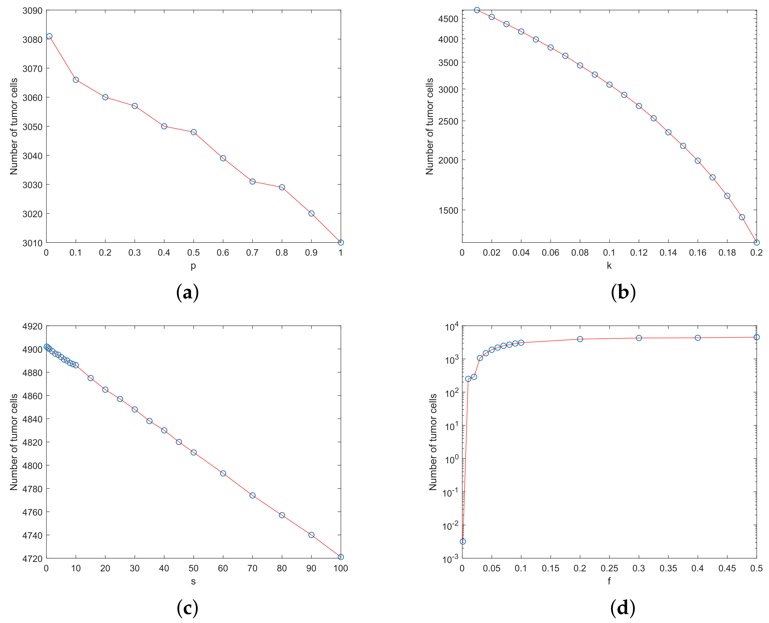
4. Parameter Sensitivity Analysis

In this section, sensitivity analysis is used to assess the impact of small parameter changes on treatment outcomes by simulating the progression of cell numbers over 25 days. We fix all the model parameter values except one parameter. By varying the parameter value to a certain range, we check the difference of model outcome to that of the model outcome using the original model parameters. Figure 2 gives the sensitivity analysis results.
In model (3), we set k = 0.1 , f = 0.1 , s = 10 , and parameter p ( 0 , 1 ) with an increment of 0.1. The initial condition is N 0 = 1 × 10 5 , L 0 = 1 × 10 2 , T 0 = 1 × 10 7 and u 0 = 10 . The simulation time period is t = 30 days. Figure 2a shows that the number of tumor cells decreases with the increase of the NK cell growth rate p. However, there are no significant changes in the number of tumor cells, which indicates that NK cells have minor effects on the output of the model. This suggests that NK cells are not as important as the CTLs to kill tumor cells.
Similarly, we fix p = 20 , f = 0.1 and s = 10 , but use k ( 0 , 0.2 ) with an increment of 0.01. Figure 2b suggests that the tumor cell number decreases if the fatality rate of tumor cells k by the chemotherapy drug increases. Figure 2b also suggests that a small variation in parameter k may have a substantial influence on the tumor cell number.
In the third test, we fix p = 20 , k = 0.1 and f = 0.1 , but s takes a value of 0 to 100. The parameter s represents the constant input of the chemotherapeutic drug. Figure 2c shows that the tumor cell number changes slightly when the drug input constant is changed. This indicates that the model is not particularly sensitive to parameter s, which suggests that we cannot achieve the therapeutic effect by increasing the drug input dose alone.
Finally, we choose p = 20 , k = 0.1 , and s = 10 , but f takes a value of 0 to 0.5, with an increment of 0.01. Figure 2d gives the number of tumor cells at t = 30 days. This figure indicates that the faster the rate of chemotherapy drug decay, the larger the number of tumor cells in the host.
Figure 2 suggests that the model is sensitive to the tumor mortality rate k induced by chemotherapy drug, as well as the drug decay rate f. These results imply that in addition to the decay rate of the chemotherapy drug, any improvement in the drug efficiency may change the treatment results substantially. Since k = k T k N , we can increase the chemotherapy drug-induced tumor mortality rate k T , or decrease the side effects of therapy drug k N . However, the tumor cell number is not very sensitive to the NK cells growth rate p and the chemotherapeutic drug input constant s. Thus, the cytolytic activity of the NK cells alone may not be a vital factor for the treatment outcomes. The activity of CTLs should also be considered.

5. Numerical Simulations

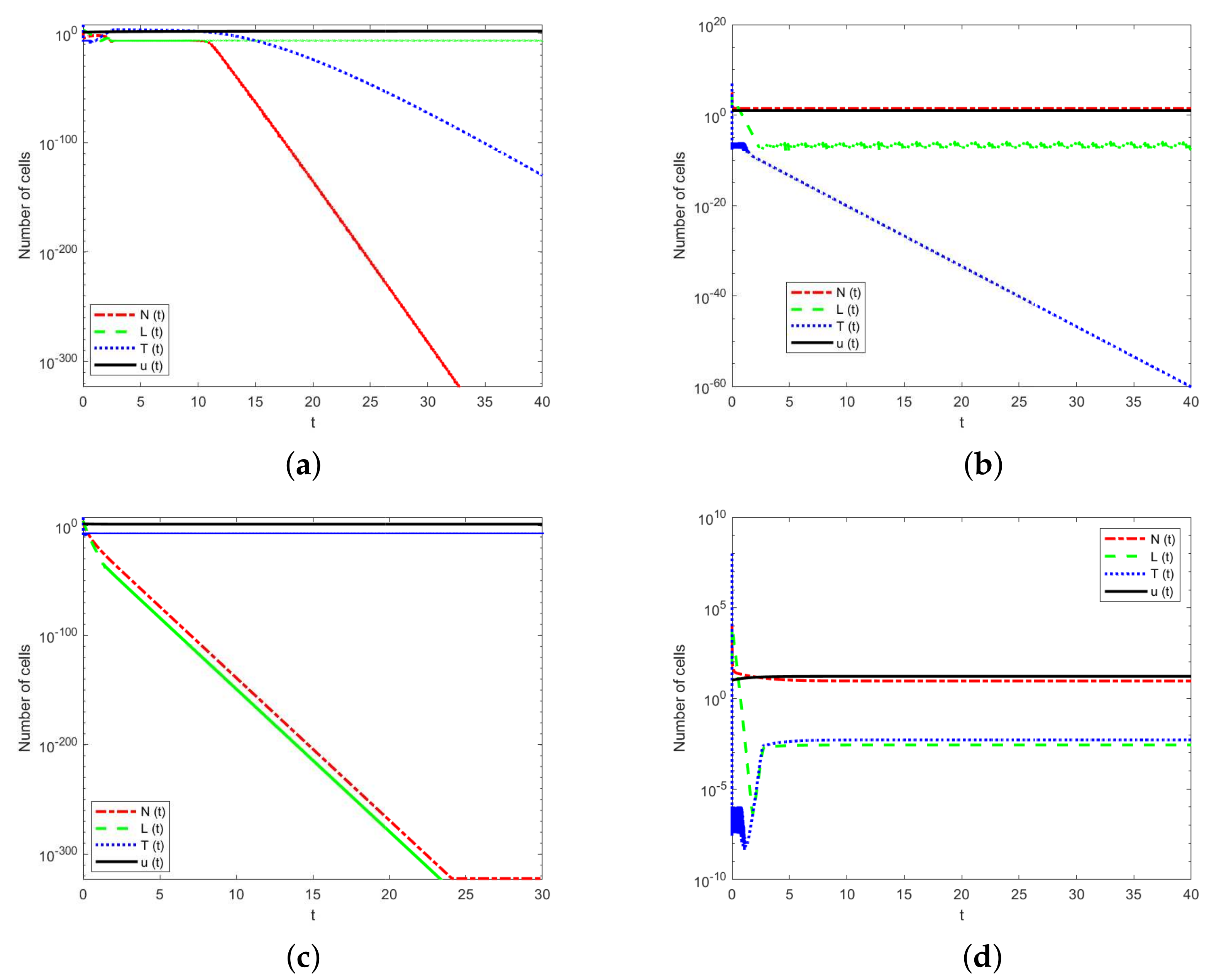
5.1. Numerical Simulations of the Equilibrium States

This subsection gives numerical simulations for the stability properties of the equilibrium states that have been proved in the previous section. The parameter values are given in Table 1 except p, k, s, and f. We use the same initial immune system strengths. Here, the parameters p, k, s, and f of each case are shown in Table 4. The initial conditions of all cases are ( N 0 , L 0 , T 0 , u 0 ) = ( 1 × 10 5 , 1 × 10 2 , 1 × 10 7 , 10 ) .
In Figure 3a, except for the drug concentration, the number of all cell populations tends to zero, that is, the equilibrium point E 0 is stable, indicating the death of the host. In Figure 3b, after a period of time, only NK cells and drugs are present, and the tumor cells are zero. Thus, the equilibrium point E 1 is stable. This is the ideal case for treatment. Figure 3c shows that only drugs and tumor cells remain, but the immune cells tend to zero. Thus, the equilibrium point E 2 is stable, which indicates that tumor cells can not be controlled by drug therapy, leading to the death of the host. Figure 3d depicts the coexistence of the immune cells and tumor cells.

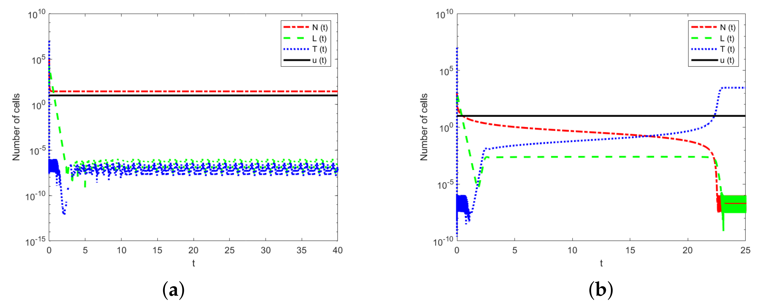
5.2. Simulations Using Different Immune Strengths

To demonstrate the effect of immune system strengths, we hypothesize that the drug has the same input constant and the same decay rate. However, different hosts have different immune system strengths. Therefore, we fix the parameter values k = 2 , f = 1 , and s = 10 . The value of parameter p is in the range of [ 10 , 20 ] . Thus, p = 20 is the strongest immune system strength, but p = 10 is the weakest one. The initial concentrations of the drug and tumor cell number are the same, namely ( T 0 , u 0 ) = ( 1 × 10 7 , 10 ) . However, the initial numbers of immune cells are different. So the initial condition in Figure 4a is N 0 = 1 × 10 5 , and L 0 = 1 × 10 2 . However, the initial condition is N 0 = 1 × 10 4 and L 0 = 1 × 10 in Figure 4b.
Figure 4 shows that different hosts with different immune system strengths have different influences on tumor cells treated with the same drug. Figure 4a shows that, after a period of treatment, only NK cells and chemotherapy drugs remain in the host. Figure 4b suggests that, under the same chemotherapeutic drug, a large number of tumor cells are present in the host when the immune system is weaker. These results suggest that a host with a stronger immune system can eliminate a small number of tumor cells under a single chemotherapy. Therefore, treatments that increase the strength of the immune system should be developed, which is a different treatment scheme (i.e., immunotherapy).

6. Discussion

Through the analysis of system equations, we determine the existence of the equilibrium points and the conditions of corresponding stability and symmetry. For a specific parameter set, we find the model may have four equilibrium states. The first one is the dead equilibrium state, which means that both immune cells and tumor cells approach zero. The second one is the tumor-free equilibrium state, in which there are only NK cells but the tumor cell number is zero. The third case is the tumor-present equilibrium state, in which there are only tumor cells in the host. The last one is the coexisting equilibrium point, which suggests that both immune and tumor cells coexist with nonzero populations. The purpose of this study is to explore the model conditions that lead to the elimination of tumor cells, namely the zero-tumor burden or tumor-free equilibrium points. Therefore, the stability of the tumor-free equilibrium is very important. The instability of the tumor-free equilibrium state means that any successful treatment must be able to alter system parameters in order to stabilize this equilibrium. However, the stability of the tumor equilibrium with a large value means that the reduction of tumor burden through chemotherapy alone is not enough to eliminate tumor cells. Once chemotherapy is stopped, the system eventually returns to the state with a large tumor number. According to the above results, the tumor-free equilibrium point E 1 is stable when parameters p and s satisfy the conditions (18) or (19). Therefore, we can change the stability of the equilibrium with zero tumor number by modifying the model parameters with chemotherapy. These results suggest a potential approach to improve the effects of chemotherapy and to design new therapy schemes.
We also analyze the sensitivity of model parameters. It should be noted that the chemotherapy drug-induced tumor mortality rate k and the drug decay rate f have the greatest influence on the treatment outcome, as seen in Figure 2. However, the number of NK cells does not have much influence on tumor growth. In addition, the cytolytic activity of the NK cells should be considered together with the CTL activity to eliminate tumor cells. Numerical simulations in Figure 3 show the importance of the host immune system and explain the side effects of chemotherapy drugs. As can be seen from the simulations in Figure 4, treatments that increase the strength of the host’s immune system should be implemented. Based on the qualitative conclusions, it is suggested to search for adjuvant treatments that increase the chemotherapy drug-induced tumor mortality rate, decrease the drug decay rate, and/or reduce the side effects of therapeutic drugs.
The main contribution of this paper is the application of two immune cell populations and chemotherapy drugs to decrease the tumor burden. However, the chemotherapeutic drug considered in our model is a constant input, which is a limitation to this study. Nevertheless, we believe that our simple model can lay the foundation for the development of more sophisticated models for tumor treatment. The future work will improve the model in this work by taking into account drug diffusion, drug-delivery methods, and drug resistance. More sophisticated models will provide more realistic simulations of tumor populations and the effects of different treatment schemes.

7. Conclusions

In conclusion, this work has extended previous mathematical models that describe tumor–immune interactions. We introduce chemotherapy into the model and propose a model to describe tumor–immune interactions under chemotherapy. We analyze the equilibrium states of the proposed model and also investigate the stability and symmetrical properties of these steady states. Sensitivity analysis is conducted to find important model parameters that have more influence on the model dynamics than other parameters. The theoretical results provide predictions for designing new treatment schemes.

Author Contributions

Conceptualization, X.Z. and T.T.; Data curation, G.S. and G.L.; Funding acquisition, X.Z.; Investigation, G.S.; Methodology, X.Z., T.T.; Software, G.S. and G.L.; Supervision, X.Z.; Validation, G.S. and G.L.; Writing–original draft, G.S., T.T. and X.Z.; Writing–review & editing, G.S., G.L., T.T. and X.Z. All authors have read and agreed to the published version of the manuscript.

Funding

This work is supported by the National Natural Science Foundation of China (No. 11871238, 11931019).

Institutional Review Board Statement

Not applicable.

Informed Consent Statement

Not applicable.

Data Availability Statement

Data sharing is not applicable to this article.

Conflicts of Interest

The authors declare no conflict of interest.

References

  1. Biemar, F.; Foti, M. Global progress against cancer-challenges and opportunities. Cancer Biol. Med. 2013, 10, 183–186. [Google Scholar] [PubMed]
  2. Bray, F.; Ferlay, J.; Soerjomataram, I.; Siegel, R.L.; Torre, L.A.; Jemal, A. Global cancer statistics 2018: Globocan estimates of incidence and mortality worldwide for 36 cancers in 185 countries. CA Cancer J. Clin. 2018, 68, 394–424. [Google Scholar] [CrossRef] [PubMed] [Green Version]
  3. Chen, W.; Zheng, R.; Baade, P.D.; Zhang, S.; Zeng, H.; Bray, F.; Jemal, A.; Yu, X.Q.; He, J. Cancer statistics in China, 2015. CA Cancer J. Clin. 2016, 66, 115–132. [Google Scholar] [CrossRef] [Green Version]
  4. Subramanian, S.; Gholami, A.; Biros, G. Simulation of glioblastoma growth using a 3D multispecies tumor model with mass effect. J. Math. Biol. 2019, 79, 941–967. [Google Scholar] [CrossRef] [Green Version]
  5. Robertson-Tessi, M.; El-Kareh, A.; Goriely, A. A model for effects of adaptive immunity on tumor response to chemotherapy and chemoimmunotherapy. J. Theor. Biol. 2015, 380, 569–584. [Google Scholar] [CrossRef]
  6. Liu, Z.; Yang, C. A mathematical model of cancer treatment by radiotherapy. Math. Comput. Simulat. 2014, 7, 172923. [Google Scholar] [CrossRef]
  7. Dakup, P.P.; Porter, K.I.; Little, A.A.; Zhang, H.; Gaddameedhi, S. Sex differences in the association between tumor growth and T cell response in a melanoma mouse model. Cancer Immunol. Immun. 2020, 69, 2157–2162. [Google Scholar] [CrossRef]
  8. Shahvaran, Z.; Kazemi, K.; Fouladivanda, M.; Helfroush, M.S.; Godefroy, O.; Aarabi, A. Morphological active contour model for automatic brain tumor extraction from multimodal magnetic resonance images. J. Neurosci. Meth. 2021, 362, 109296. [Google Scholar] [CrossRef]
  9. Pang, L.; Lin, S.; Zhong, Z. Mathematical modelling and analysis of the tumor treatment regimens with pulsed immunotherapy and chemotherapy. Comput. Math. Methods Med. 2016, 2016, 6260474. [Google Scholar] [CrossRef] [Green Version]
  10. Neoptolemos, J. A randomized trial of chemoradiotherapy and chemotherapy after resection of pancreatic cancer. N. Engl. J. Med. 2016, 350, 1200. [Google Scholar] [CrossRef] [Green Version]
  11. López, A.G.; Seoane, J.M.; Sanjuán, M.A.F. A validated mathematical model of tumor growth including tumor-host interaction, cell-mediated immune response and chemotherapy. Bull. Math. Biol. 2014, 76, 2884–2906. [Google Scholar] [CrossRef] [PubMed]
  12. Shu, Y.; Huang, J.; Dong, Y.; Takeuchi, Y. Mathematical modeling and bifurcation analysis of pro- and anti-tumor macrophages. Appl. Math. Mol. 2020, 88, 758–773. [Google Scholar] [CrossRef]
  13. Roesch, K.; Hasenclever, D.; Scholz, M. Modelling Lymphoma Therapy and Outcome. Bull. Math. Biol. 2014, 76, 401–430. [Google Scholar] [CrossRef] [PubMed] [Green Version]
  14. Murray, I.; Du, Y. Systemic radiotherapy of bone metastases with radionuclides. Clin. Oncol. 2021, 33, 98–105. [Google Scholar] [CrossRef]
  15. Glatzer, M.; Faivre-Finn, C.; Ruysscher, D.D.; Widder, J.; Van Houtte, P.; Troost, E.G.; Slotman, B.J.; Ramella, S.; Pöttgen, C.; Peeters, S.T.H.; et al. Role of radiotherapy in the management of brain metastases of NSCLC-Decision criteria in clinical routine. Radiother. Oncol. 2021, 154, 269–273. [Google Scholar] [CrossRef]
  16. Mulemba, T.; Bank, R.; Sabantini, M.; Chopi, V.; Chirwa, G.; Mumba, S.; Chasela, M.; Lemon, S.; Hockenberry, M. Improving peripheral intravenous catheter care for children with cancer receiving chemotherapy in Malawi. J. Pediatr. Nurs. 2021, 56, 13–17. [Google Scholar] [CrossRef]
  17. Dagher, O.; King, T.R.; Wellhausen, N.; Posey, A.D. Combination Therapy for Solid Tumors: Taking a Classic CAR on New Adventures. Cancer Cell 2020, 38, 621–623. [Google Scholar] [CrossRef]
  18. Magee, D.E.; Hird, A.E.; Klaassen, Z.; Sridhar, S.S.; Nam, R.K.; Wallis, C.J.D.; Kulkarni, G.S. Adverse event profile for immunotherapy agents compared with chemotherapy in solid organ tumors: A systematic review and meta-analysis of randomized clinical trials. Ann. Oncol. 2020, 31, 50–60. [Google Scholar] [CrossRef] [Green Version]
  19. Abernathy, Z.; Abernathy, K.; Stevens, J. A mathematical model for tumor growth and treatment using virotherapy. AIMS Math. 2020, 5, 4136–4150. [Google Scholar] [CrossRef]
  20. Mongkolkeha, C.; Dhananjay, G. Some common fixed point theorems for eneralized F-contraction involving w-distance with some applications to differential qquations. Mathematics 2019, 7, 32. [Google Scholar] [CrossRef] [Green Version]
  21. Yousef, A.; Bozkurt, F.; Abdeljawad, T. Mathematical modeling of the immune-chemotherapeutic treatment of breast cancer under some control parameters. Adv. Differ. Equ. 2020, 2020, 696. [Google Scholar] [CrossRef]
  22. Kumar, D.R. Common fixed point results under w-distance with applications to nonlinear integral equations and nonlinear fractional differential equations. Math. Slovaca 2021, 71, 1511–1528. [Google Scholar] [CrossRef]
  23. Guran, L.; Mitrović, Z.D.; Reddy, G.S.M.; Belhenniche, A.; Radenović, S. Applications of a fixed point result for solving nonlinear fractional and integral differential equations. Fractal Fract. 2021, 5, 211. [Google Scholar] [CrossRef]
  24. Sarkar, S.; Sahoo, P.K.; Mahata, S.; Pal, R.; Ghosh, D.; Mistry, T.; Ghosh, S.; Bera, T.; Nasare, V.D. Mitotic checkpoint defects: En route to cancer and drug resistance. Chromosome Res. 2021, 12, 131–144. [Google Scholar] [CrossRef]
  25. Feizabadi, M.S. Modeling multi-mutation and drug resistance: Analysis of some case studies. Theor. Biol. Med. Model. 2017, 14, 275–289. [Google Scholar] [CrossRef] [PubMed] [Green Version]
  26. Cen, X.; Feng, Z.; Zheng, Y.; Zhao, Y. Bifurcation analysis and global dynamics of a mathematical model of antibiotic resistance in hospitals. J. Math. Biol. 2017, 75, 1463–1485. [Google Scholar] [CrossRef] [PubMed] [Green Version]
  27. Song, G.; Tian, T.; Zhang, X. A mathematical model of cell-mediated immune response to tumor. Math. Biosci. Eng. 2021, 18, 373–385. [Google Scholar] [CrossRef]
  28. Yan, Y.; Jiang, F.; Zhang, X.; Tian, T. Integrated inference of asymmetric protein interaction networks using dynamic model and individual patient proteomics data. Symmetry 2021, 13, 1097. [Google Scholar] [CrossRef]
  29. Li, L.; Shao, M.; He, X.; Ren, S.; Tian, T. Risk of lung cancer due to external environmental factor and epidemiological data analysis. Math. Biosci. Eng. 2021, 18, 6079–6094. [Google Scholar] [CrossRef]
  30. Amer, A.; Nagah, A.; Tian, T.; Zhang, X. Mutation mechanisms of breast cancer among the female population in China. Curr. Bioinform. 2020, 15, 253–259. [Google Scholar] [CrossRef]
  31. Pang, L.; Liu, S.; Zhang, X.; Tian, T. Mathematical modeling and dynamic analysis of anti-tumor immune response. J. Appl. Math. Comput. 2020, 62, 473–488. [Google Scholar] [CrossRef]
  32. Li, L.; Tian, T.; Zhang, X. Stochastic modelling of multistage carcinogenesis and progression of human lung cancer. J. Theor. Biol. 2019, 479, 81–89. [Google Scholar] [CrossRef] [PubMed]
  33. Diefenbach, A.; Jensen, E.; Jamieson, A.; Raulet, D.H. Rae1 and H60 ligands of the NKG2D receptor stimulate tumor immunity. Theor. Nat. 2001, 413, 165–171. [Google Scholar]
  34. Yates, A.; Callard, R. Cell death and the maintenance of immunological memory. Discret. Contin. Dyn. Syst.-B 2002, 1, 43–59. [Google Scholar] [CrossRef]
  35. Lanzavecchia, A.; Sallusto, F. Dynamics of T lymphocyte responses: Intermediates, effectors, and memory cells. Science 2000, 290, 92–97. [Google Scholar] [CrossRef]
  36. Dudley, M.E.; Wunderlich, J.R.; Robbins, P.F.; Yang, J.C.; Hwu, P.; Schwartzentruber, D.J.; Topalian, S.L.; Sherry, R.; Restifo, N.P.; Hubicki, A.M.; et al. Cancer regression and autoimmunity in patients after clonal repopulation with antitumor lymphocytes. Science 2002, 298, 850–854. [Google Scholar] [CrossRef] [Green Version]
  37. Delisi, C.; Rescigno, A. Immune surveillance and neoplasia. I. A minimal mathematical model. Bull. Math. Biol. 1977, 39, 201–221. [Google Scholar]
  38. Chen, L. Mathematical Models and Methods in Ecology; Science Press: Beijing, China, 1988; pp. 174–198. (In Chinese) [Google Scholar]
Figure 1. Model assumptions about the detailed interactions between tumor cells, the immune system, and chemotherapy.
Symmetry 14 00704 g001
Figure 2. Sensitivity analysis of model (3) by changing the values of four parameters. (a) Parameter p. (b) Parameter k. (c) Parameter s. (d) Parameter f.
Symmetry 14 00704 g002
Figure 3. Numerical simulations of the model for four equilibrium states. (a). Dead equilibrium state E 0 . (b) Tumor–free equilibrium state E 1 . (c) Tumor–present equilibrium state E 2 . (d) Coexisting equilibrium state E 3 .
Symmetry 14 00704 g003
Figure 4. The numbers of tumor cells and immune cells under chemotherapy with different immune intensities. (a) Simulation using a strong immune system strength with p = 20 . (b) Simulation using a weak immune system strength with p = 10 .
Symmetry 14 00704 g004
Table 1. Description and values of the parameters in model (1).
ParametersUnitsDescriptionValueReference
aday 1 Growth rate of NK cellsnonenone
bcell 1 Inverse of NK cells capacity 3.17 × 10 6 fitting
cday 1 Growth rate of tumor 5.14 × 10 1  [33]
dcell 1 Inverse of tumor capacity 1.02 × 10 9  [33]
rcell 1 day 1 Activation rate of CTLs 1.1 × 10 7  [34,35]
μ day 1 CTL death rate 2.0 × 10 2  [34]
α 1 cell 1 day 1 NK cell death rate 1.0 × 10 7  [33]
α 2 cell 1 day 1 Tumor death rate of NK 6.41 × 10 11  [33,36]
β 1 cell 1 day 1 CTL death rate 3.42 × 10 10  [37]
β 2 cell 1 day 1 Rate of CTL-induced tumor death 3.5 × 10 7 fitting
vdoseInflux of drugnonenone
ω day 1 Drug decay rate 9 × 10 1  [12]
k N , k L day 1 Immune cell killed by drug 6 × 10 1  [12]
k T day 1 Tumor cell killed by drug 8 × 10 1 [12]
Table 2. Endemic equilibrium states of model (3) and the corresponding parameter ranges.
No.pkfEquilibrium Points
1 2.92 × 10 4 ( 5.23 × 10 3 ,  + ) ( f 1 ,   + ) E 3 ( N 1 , L 1 , T 1 , s f )
2 ( 1.23 × 10 4 , 2.92 × 10 4 ) ( 0 , 1 1.8 × 10 2 p ) ( 0 , f 3 ) E 3 ( N 2 , L 2 , T 2 , s f )
3 ( 0 , 5.06 × 10 3 ) ( 0 , k 1 ) ( f 2 ,   + ) E 3 ( N 3 , L 3 , T 3 , s f )
Table 3. The existence of equilibrium states of model (3) ( s ( 0 , + ) ).
No.pkfEquilibrium Points
1 ( 0 , + ) ( 0 , + ) ( 0 , + ) E 0 ( 0 , 0 , 0 , s f )
2 ( s f , + ) ( 0 , + ) ( 0 , + ) E 1 ( p s f 1.8 × 10 2 p , 0 , 0 , s f )
3 ( 0 , + ) ( 0 , + ) ( k s 25.7 , + ) E 2 ( 0 , 0 , 1.91 × 10 2 ( 25.7 k s f ) , s f )
4 2.92 × 10 4 ( 5.23 × 10 3 , + ) ( f 1 , + ) E 3 ( N 1 , L 1 , T 1 , s f )
5 ( 1.23 × 10 4 , 2.92 × 10 4 ) ( 0 , 1 1.8 × 10 2 p ) ( 0 , f 3 ) E 3 ( N 2 , L 2 , T 2 , s f )
6 ( 0 , 5.06 × 10 3 ) ( 0 , k 1 ) ( f 2 , + ) E 3 ( N 3 , L 3 , T 3 , s f )
Table 4. The values of the fixed parameter p, k, s, and f for each simulation graph.
No.pksfEquilibrium Points
110 0.4 10 0.1 E 0
210101 0.1 E 1
320 0.1 10 0.2 E 2
420 0.01 10 0.6 E 3
Publisher’s Note: MDPI stays neutral with regard to jurisdictional claims in published maps and institutional affiliations.

