Heisenberg Parabolic Subgroups of Exceptional Non-Compact G₂₍₂₎ and Invariant Differential Operators

Abstract

In the present paper we continue the project of systematic construction of invariant differential operators on the example of the non-compact algebra $G_{2\left(2\right)}$. We use both the minimal and the maximal Heisenberg parabolic subalgebras. We give the main multiplets of indecomposable elementary representations. This includes the explicit parametrization of the intertwining differential operators between the ERs. These are new results applicable in all cases when one would like to use $G_{2\left(2\right)}$ invariant differential operators.

1. Introduction

Invariant differential operators play very important role in the description of physical symmetries. In a recent paper [1] we started the systematic explicit construction of invariant differential operators. We gave an explicit description of the building blocks, namely the parabolic subgroups and subalgebras from which the necessary representations are induced. Thus, we have set the stage for study of different non-compact groups. An update of the developments as of 2016 is given in [2] (see also [3]).

In the present paper we focus on the exceptional non-compact algebra $G_{2\left(2\right)}$. Below we give the general preliminaries necessary for our approach. In Section 2 we introduce the Lie algebra $G_2$ (following [4]), its real from $G_{2\left(2\right)}$ and, shortly, the corresponding Lie group. In Section 3 we consider the representations induced from the minimal parabolic subalgebra of $G_{2\left(2\right)}$. In Section 4 we consider the representations induced from the two maximal Heisenberg parabolic subalgebras of $G_{2\left(2\right)}$.

Preliminaries

Let G be a semi-simple non-compact Lie group, and K a maximal compact subgroup of G. Then we have an Iwasawa decomposition $G=K{A}_0{N}_0$, where $A_0$ is an abelian simply connected vector subgroup of G, and $N_0$ is a nilpotent simply connected subgroup of G preserved by the action of $A_0$. Further, let $M_0$ be the centralizer of $A_0$ in K. Then the subgroup $P_0=M_0{A}_0{N}_0$ is a minimal parabolic subgroup of G. A parabolic subgroup $P=MAN$ is any subgroup of G which contains a minimal parabolic subgroup.

The importance of the parabolic subgroups comes from the fact that the representations induced from them generate all (admissible) irreducible representations of G [5,6,7]. Actually, it may happen that there are overlaps which should be taken into account.

Let $\nu$ be a (non-unitary) character of A, $\nu \in {\mathcal{A}}^{\ast }$, let $\mu$ fix an irreducible representation $D^{\mu }$ of M on a vector space $V_{\mu }$.

We call the induced representation $\chi =$ Ind${}_P^G(\mu \otimes \nu \otimes 1)$ an elementary representation of G [8]. (In the mathematical literature these representations are called “generalised principal series representations”, cf., e.g., [9].) Their spaces of functions are:

$${\mathcal{C}}_{\chi }=\{\mathcal{F}\in C^{\infty }(G,V_{\mu })|\mathcal{F}\left(gman\right)=e^{-\nu \left(H\right)}·D^{\mu }\left(m^{-1}\right)\mathcal{F}\left(g\right)\}$$

(1)

where $a=exp\left(H\right)\in A$, $H\in \mathcal{A}$, $m\in M$, $n\in N$. The representation action is the $left$ regular action:

$$\left({\mathcal{T}}^{\chi }\left(g\right)\mathcal{F}\right)\left(g^{\prime }\right)=\mathcal{F}\left(g^{-1}{g}^{\prime }\right),g,g^{\prime }\in G.$$

(2)

An important ingredient in our considerations are the Verma modules $V^{\mathrm{\Lambda }}$ over ${\mathcal{G}}^{\mathbb{C}}$, where $\mathrm{\Lambda }\in ({{\mathcal{H}}^{\mathbb{C}})}^{\ast }$, ${\mathcal{H}}^{\mathbb{C}}$ is a Cartan subalgebra of ${\mathcal{G}}^{\mathbb{C}}$, the weight $\mathrm{\Lambda }=\mathrm{\Lambda }\left(\chi \right)$ is determined uniquely from $\chi$ [10,11].

Actually, since our ERs will be induced from finite-dimensional representations of $\mathcal{M}$ (or their limits) the Verma modules are always reducible. Thus, it is more convenient to use generalized Verma modules ${\tilde{V}}^{\mathrm{\Lambda }}$ such that the role of the highest/lowest weight vector $v_0$ is taken by the space $V_{\mu }{v}_0$. For the generalized Verma modules (GVMs) the reducibility is controlled only by the value of the conformal weight d (related to $\nu$, see below). Relatedly, for the intertwining differential operators only the reducibility w.r.t. non-compact roots is essential.

One main ingredient of our approach is as follows. We group the (reducible) ERs with the same Casimirs in sets called multiplets [11,12]. The multiplet corresponding to fixed values of the Casimirs may be depicted as a connected graph, the vertices of which correspond to the reducible ERs, and the lines between the vertices correspond to intertwining operators. The explicit parametrization of the multiplets and of their ERs is important for understanding of the situation.

In fact, the multiplets explicitly contain all the data necessary to construct the intertwining differential operators. Actually, the data for each intertwining differential operator consists of the pair $(\beta ,m)$, where $\beta$ is a (non-compact) positive root of ${\mathcal{G}}^{\mathbb{C}}$, $m\in IN$, such that the BGG [13] Verma module reducibility condition (for highest weight modules) is fulfilled:

$$(\mathrm{\Lambda }+\rho ,{\beta }^{\vee })=m,{\beta }^{\vee }\equiv 2\beta /(\beta ,\beta ).$$

(3)

when (3) then holds the Verma module with shifted weight $V^{\mathrm{\Lambda }-m\beta }$ (or ${\tilde{V}}^{\mathrm{\Lambda }-m\beta }$ for GVM and $\beta$ non-compact) is embedded in the Verma module $V^{\mathrm{\Lambda }}$ (or ${\tilde{V}}^{\mathrm{\Lambda }}$). This embedding is realized by a singular vector $v_s$ determined by a polynomial ${\mathcal{P}}_{m,\beta }\left({\mathcal{G}}^{-}\right)$ in the universal enveloping algebra $\left(U\left({\mathcal{G}}_{-}\right)\right)v_0$, ${\mathcal{G}}^{-}$ is the subalgebra of ${\mathcal{G}}^{\mathbb{C}}$ generated by the negative root generators [14]. More explicitly, [11], $v_{m,\beta }^s={\mathcal{P}}_{\beta }^m{v}_0$ (or $v_{m,\beta }^s={\mathcal{P}}_{\beta }^m{V}_{\mu }{v}_0$ for GVMs). Then there exists [11] an intertwining differential operator

$${\mathcal{D}}_{\beta }^m:{\mathcal{C}}_{\chi \left(\mathrm{\Lambda }\right)}⟶{\mathcal{C}}_{\chi (\mathrm{\Lambda }-m\beta )}$$

(4)

given explicitly by:

$${\mathcal{D}}_{\beta }^m={\mathcal{P}}_{\beta }^m\left(\widehat{{\mathcal{G}}^{-}}\right)$$

(5)

where $\widehat{{\mathcal{G}}^{-}}$ denotes the $right$ action on the functions $\mathcal{F}$, cf. (1).

2. The Non-Compact Lie Group and Algebra of Type ${\mathit{G}}_{\mathbf{2}}$

Let ${\mathcal{G}}^{\mathbb{C}}=G_2$, with Cartan matrix: $\left(a_{ij}\right)=\left(\begin{array}{cc}2& -3\\ -1& 2\end{array}\right)$, simple roots ${\alpha }_1,{\alpha }_2$ with products: $({\alpha }_2,{\alpha }_2)=3({\alpha }_1,{\alpha }_1)=-2({\alpha }_2,{\alpha }_1)$. We choose $({\alpha }_1,{\alpha }_1)=2$, then $({\alpha }_2,{\alpha }_2)=6$, $({\alpha }_2,{\alpha }_1)=-3$. (Note that in [4] we have chosen ${\alpha }_1$ as the long root, and ${\alpha }_2$ as the short root). As we know $G_2$ is 14-dimensional. The positive roots may be chosen as:

$${\Delta }^{+}=\{{\alpha }_1,{\alpha }_2,{\alpha }_1+{\alpha }_2,{\alpha }_2+2{\alpha }_1,{\alpha }_2+3{\alpha }_1,2{\alpha }_2+3{\alpha }_1\}$$

(6)

We shall use the orthonormal basis ${\epsilon }_1,{\epsilon }_2,{\epsilon }_3$. In its terms the positive roots are given as:

$$\begin{array}{ccc}& & {\alpha }_1={\epsilon }_1-{\epsilon }_2,{\alpha }_3={\alpha }_1+{\alpha }_2={\epsilon }_2-{\epsilon }_3,{\alpha }_4={\alpha }_2+2{\alpha }_1={\epsilon }_1-{\epsilon }_3\hfill \end{array}$$

(7a)

$$\begin{array}{ccc}& & {\alpha }_2=-{\epsilon }_1+2{\epsilon }_2-{\epsilon }_3,{\alpha }_5={\alpha }_2+3{\alpha }_1=2{\epsilon }_1-{\epsilon }_2-{\epsilon }_3,\hfill \\ & & {\alpha }_6=2{\alpha }_2+3{\alpha }_1={\epsilon }_1+{\epsilon }_2-2{\epsilon }_3\hfill \end{array}$$

(7b)

where, for future reference, we have also introduced notation for the non-simple roots. (Note that in (7a) are the short roots, in (7b) are the long roots.)

Another way to write the roots in general is $\beta =(b_1,b_2,b_3)$ under the condition $b_1+b_2+b_3=0$. Then:

$$\begin{array}{ccc}\hfill & & {\alpha }_1=(1,-1,0),{\alpha }_2+{\alpha }_1=(0,1,-1),{\alpha }_2+2{\alpha }_1=(1,0,-1)\hfill \\ & & {\alpha }_2=(-1,2,-1),{\alpha }_2+3{\alpha }_1=(2,-1,-1),2{\alpha }_2+3{\alpha }_1=(1,1,-2)\hfill \end{array}$$

(8)

The dual roots are: ${\alpha }_1^{\vee }={\alpha }_1$, ${\alpha }_2^{\vee }={\alpha }_2/3$, ${({\alpha }_2+{\alpha }_1)}^{\vee }={\alpha }_2+{\alpha }_1=3{\alpha }_2^{\vee }+{\alpha }_1^{\vee }$, ${({\alpha }_2+2{\alpha }_1)}^{\vee }={\alpha }_2+2{\alpha }_1=3{\alpha }_2^{\vee }+2{\alpha }_1^{\vee }$, ${({\alpha }_2+3{\alpha }_1)}^{\vee }=({\alpha }_2+3{\alpha }_1)/3={\alpha }_2^{\vee }+{\alpha }_1^{\vee }$, ${(2{\alpha }_2+3{\alpha }_1)}^{\vee }=(2{\alpha }_2+3{\alpha }_1)/3=2{\alpha }_2^{\vee }+{\alpha }_1^{\vee }$.

The Weyl group $W({\mathcal{G}}^{\mathbb{C}},{\mathcal{H}}^{\mathbb{C}})$ of $G_2$ is the dihedral group of order 12. This follows from the fact that ${\left(s_1{s}_2\right)}^6=1$, where $s_1,s_2$ are the two simple reflections.

The complex Lie algebra $G_2$ has one non-compact real form: $\mathcal{G}=G_{2\left(2\right)}$ which is naturally split. Its maximal compact subalgebra is $\mathcal{K}=su\left(2\right)\oplus su\left(2\right)$, also written as $\mathcal{K}=su{\left(2\right)}_S\oplus su{\left(2\right)}_L$ to emphasize the relation to the root system (after complexification the first factor contains a short root, the second—a long root). We remind that $\mathcal{G}=G_{2\left(2\right)}$ has discrete series representations. Actually, it is quaternionic discrete series since $\mathcal{K}$ contains as direct summand (at least one) $su\left(2\right)$ subalgebra. The number of discrete series is equal to the ratio $|W({\mathcal{G}}^{\mathbb{C}},{\mathcal{H}}^{\mathbb{C}})|/|W({\mathcal{K}}^{\mathbb{C}},{\mathcal{H}}^{\mathbb{C}})|$, where $\mathcal{H}$ is a compact Cartan subalgebra of both $\mathcal{G}$ and $\mathcal{K}$, W are the relevant Weyl groups [9]. Thus, the number of discrete series in our setting is three. They will be identified below.

The compact Cartan subalgebra $\mathcal{H}$ of $\mathcal{G}$ will be chosen (following [15]) to coincide with the Cartan subalgebra of $\mathcal{K}$ and we may write: $\mathcal{H}=u{\left(1\right)}_S\oplus u{\left(1\right)}_L$. (One may write as in [15] $\mathcal{H}={\mathcal{T}}_1\oplus {\mathcal{T}}_2$ to emphasize the torus nature.) Accordingly, we choose for the positive root system of ${\mathcal{K}}^{\mathbb{C}}$ the roots ${\alpha }_1+{\alpha }_2=(0,1,-1)$, and ${\alpha }_2+3{\alpha }_1=(2,-1,-1)$ (which are orthogonal to each other). The lattice of characters of $\mathcal{H}$ is ${\lambda }_{\mathcal{H}}=\frac{1}{2}\mu ({\alpha }_1+{\alpha }_2)+\frac{1}{2}\nu ({\alpha }_2+3{\alpha }_1)$, where $\mu ,\nu \in \mathbb{Z}$.

The complimentary to $\mathcal{K}$ space is $\mathcal{Q}$ and it is eight-dimensional.

The Iwasawa decomposition of $\mathcal{G}$ is:

$$\begin{array}{ccc}\hfill \mathcal{G}& =& \mathcal{K}\oplus {\mathcal{A}}_0\oplus {\mathcal{N}}_0\hfill \\ & & dim{\mathcal{A}}_0=2,dim{\mathcal{N}}_0=6\hfill \end{array}$$

(9)

The Bruhat decomposition is:

$$\begin{array}{ccc}\hfill \mathcal{G}& =& {\tilde{\mathcal{N}}}_0\oplus {\mathcal{M}}_0\oplus {\mathcal{A}}_0\oplus {\mathcal{N}}_0\hfill \\ & & {\mathcal{M}}_0=0,dim{\tilde{\mathcal{N}}}_0=6\hfill \end{array}$$

(10)

Accordingly the minimal parabolic of $\mathcal{G}$ is:

$${\mathcal{P}}_0={\mathcal{M}}_0\oplus {\mathcal{A}}_0\oplus {\mathcal{N}}_0={\mathcal{A}}_0\oplus {\mathcal{N}}_0$$

(11)

There are two isomorphic maximal cuspidal parabolic subalgebras of $\mathcal{G}$ which are of Heisenberg type:

$$\begin{array}{ccc}\hfill & & {\mathcal{P}}_k={\mathcal{M}}_k\oplus {\mathcal{A}}_k\oplus {\mathcal{N}}_k,k=1,2;\hfill \\ & & {\mathcal{M}}_k=sl{(2,IR)}_k,dim{\mathcal{A}}_k=1,dim{\mathcal{N}}_k=5\hfill \end{array}$$

(12)

Let us denote by ${\mathcal{T}}_k$ the compact Cartan subalgebra of ${\mathcal{M}}_k$. (Recall that $[{\mathcal{M}}_j,{\mathcal{A}}_k]=0$ for $j\ne k$.) Then ${\mathcal{H}}_k={\mathcal{T}}_k\oplus {\mathcal{A}}_k$ is a non-compact Cartan subalgebra of $\mathcal{G}$. We choose ${\mathcal{T}}_1$ to be generated by the short $\mathcal{K}$-compact root ${\alpha }_1+{\alpha }_2$ and ${\mathcal{A}}_1$ to be generated by the long root ${\alpha }_2$, while ${\mathcal{T}}_2$ is chosen to be generated by the long $\mathcal{K}$-compact root ${\alpha }_2+3{\alpha }_1$ and ${\mathcal{A}}_2$ is chosen to be generated by the short root ${\alpha }_1$.

Equivalently, the ${\mathcal{M}}_1$-compact root of ${\mathcal{G}}^{\mathbb{C}}$ is ${\alpha }_1+{\alpha }_2$, while the ${\mathcal{M}}_2$-compact root is ${\alpha }_2+3{\alpha }_1$. In each case the remaining five positive roots of ${\mathcal{G}}^{\mathbb{C}}$ are ${\mathcal{M}}_k$-non-compact.

To characterize the Verma modules we shall first use the Dynkin labels:

$$m_i\equiv (\mathrm{\Lambda }+\rho ,{\alpha }_i^{\vee }),i=1,2,$$

(13)

where $\rho$ is half the sum of the positive roots of ${\mathcal{G}}^{\mathbb{C}}$. Thus, we shall use:

$${\chi }_{\mathrm{\Lambda }}=\{m_1,m_2\}$$

(14)

Note that when both $m_i\in IN$ then ${\chi }_{\mathrm{\Lambda }}$ characterizes the finite-dimensional irreps of ${\mathcal{G}}^{\mathbb{C}}$ and its real forms, in particular, $\mathcal{G}$. Furthermore, $m_k\in IN$ characterizes the finite-dimensional irreps of the ${\mathcal{M}}_k$ subalgebra.

We shall use also the Harish-Chandra parameters:

$$m_{\beta }=(\mathrm{\Lambda }+\rho ,{\beta }^{\vee }),$$

(15)

for any positive root $\beta$, and explicitly in terms of the Dynkin labels:

$$\begin{array}{ccc}\hfill {\chi }_{HC}& =& \{m_1,m_3=3m_2+m_1,m_4=3m_2+2m_1\hfill \end{array}$$

(16a)

$$\begin{array}{ccc}& & m_2,m_5=m_2+m_1,m_6=2m_2+m_1,\}\hfill \end{array}$$

(16b)

3. Induction from Minimal Parabolic

3.1. Main Multiplets

The main multiplets are in 1-to-1 correspondence with the finite-dimensional irreps of $G_2$, i.e., they are labeled by the two positive Dynkin labels $m_i\in IN$. When we induce from the minimal parabolic the main multiplets of $\mathcal{G}$ are the same as for the complexified Lie algebra ${\mathcal{G}}^{\mathbb{C}}$. The latter were considered in [4] but here we give a different parametrization.

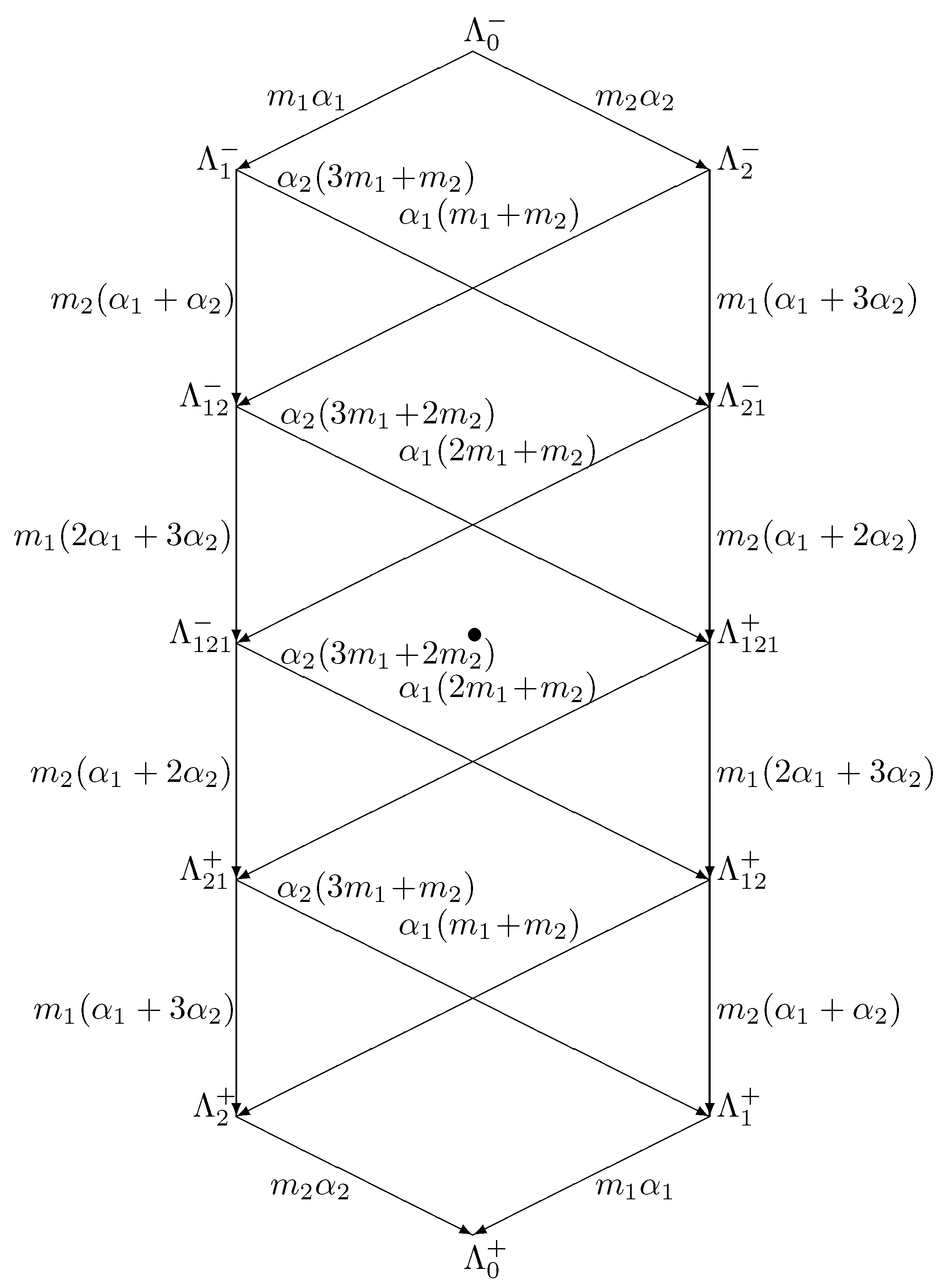
We take ${\chi }_0={\chi }_{HC}$. It has two embedded Verma modules with HW ${\mathrm{\Lambda }}_1={\mathrm{\Lambda }}_0-m_1{\alpha }_1$, and ${\mathrm{\Lambda }}_2={\mathrm{\Lambda }}_0-m_2{\alpha }_2$. The number of ERs/GVMs in a main multiplet is $12=|W({\mathcal{G}}^{\mathbb{C}})|$. We give the whole multiplet as follows:

$$\begin{array}{ccc}\hfill {\chi }_0& =& \{m_1,m_2;-\frac{1}{2}(2m_2+m_1)\}\hfill \\ \hfill {\chi }_2& =& \{3m_2+m_1,-m_2;-\frac{1}{2}(m_2+m_1)\},{\mathrm{\Lambda }}_2={\mathrm{\Lambda }}_0-m_2{\alpha }_2\hfill \\ \hfill {\chi }_1& =& \{-m_1,m_2+m_1;-\frac{1}{2}(2m_2+m_1)\},{\mathrm{\Lambda }}_1={\mathrm{\Lambda }}_0-m_1{\alpha }_1\hfill \\ \hfill {\chi }_{21}& =& \{3m_2+2m_1,-m_2-m_1;-\frac{1}{2}{m}_2\},{\mathrm{\Lambda }}_{21}={\mathrm{\Lambda }}_2-m_1{\alpha }_3\hfill \\ \hfill {\chi }_{12}& =& \{-3m_2-m_1,2m_2+m_1;-\frac{1}{2}(m_2+m_1)\},{\mathrm{\Lambda }}_{12}={\mathrm{\Lambda }}_1-m_2{\alpha }_5\hfill \\ \hfill {\chi }_{212}& =& \{3m_2+2m_1,-2m_2-m_1;\frac{1}{2}{m}_2\},{\mathrm{\Lambda }}_{212}={\mathrm{\Lambda }}_0-(m_1+3m_2){\alpha }_3\hfill \\ \hfill {\chi }_{121}& =& \{-3m_2-2m_1,2m_2+m_1;-\frac{1}{2}{m}_2\},{\mathrm{\Lambda }}_{121}={\mathrm{\Lambda }}_0-(m_1+m_2){\alpha }_5\hfill \\ \hfill {\chi }_{2121}& =& \{3m_2+m_1,-2m_2-m_1;\frac{1}{2}(m_2+m_1)\},{\mathrm{\Lambda }}_{2121}={\mathrm{\Lambda }}_{212}-m_1{\alpha }_4\hfill \\ \hfill {\chi }_{1212}& =& \{-3m_2-2m_1,m_2+m_1;\frac{1}{2}{m}_2\},{\mathrm{\Lambda }}_{1212}={\mathrm{\Lambda }}_{121}-m_2{\alpha }_6\hfill \\ \hfill {\chi }_{21212}& =& \{m_1,-m_2-m_1;\frac{1}{2}(2m_2+m_1)\},{\mathrm{\Lambda }}_{21212}={\mathrm{\Lambda }}_0-(m_1+2m_2){\alpha }_6\hfill \\ \hfill {\chi }_{12121}& =& \{-3m_2-m_1,m_2;\frac{1}{2}(m_2+m_1)\},{\mathrm{\Lambda }}_{12121}={\mathrm{\Lambda }}_0-(2m_1+3m_2){\alpha }_4\hfill \\ \hfill {\chi }_{121212}& =& \{-m_1,-m_2;\frac{1}{2}(2m_2+m_1)\}={\chi }_{212121}={\left(s_1{s}_2\right)}^3·{\mathrm{\Lambda }}_0={\left(s_2{s}_1\right)}^3·{\mathrm{\Lambda }}_0,\hfill \end{array}$$

(17)

where we have also included, as the third entry, the parameter $c=-\frac{1}{2}(2m_2+m_1)$, related to the Harish-Chandra parameter of the highest root (recalling that $m_{{\alpha }_6}=2m_2+m_1$). It is also related to the conformal weight $d=\frac{3}{2}+c$.

Using this labeling, the signatures may be given in the following pair-wise manner:

$$\begin{array}{ccc}\hfill {\chi }_0^{\pm }& =& \{\mp m_1,\mp m_2;\pm \frac{1}{2}(2m_2+m_1)\}\hfill \\ \hfill {\chi }_2^{\pm }& =& \{\mp (3m_2+m_1),\pm m_2;\pm \frac{1}{2}(m_2+m_1)\},\hfill \\ \hfill {\chi }_1^{\pm }& =& \{\pm m_1,\mp (m_2+m_1);\pm \frac{1}{2}(2m_2+m_1)\},\hfill \\ \hfill {\chi }_{12}^{\pm }& =& \{\mp (3m_2+2m_1),\pm (m_2+m_1);\pm \frac{1}{2}{m}_2\}\hfill \\ \hfill {\chi }_{21}^{\pm }& =& \{\pm (3m_2+m_1),\mp (2m_2+m_1);\pm \frac{1}{2}(m_2+m_1)\}\hfill \\ \hfill {\chi }_{121}^{\pm }& =& \{\mp (3m_2+2m_1),\pm (2m_2+m_1);\mp \frac{1}{2}{m}_2\},\hfill \end{array}$$

(18)

where ${\chi }_{\dots }^{-}={\chi }_{\dots }$ from (17), ${\chi }_0^{+}={\chi }_{121212}$, ${\chi }_1^{+}={\chi }_{21212}$, ${\chi }_2^{+}={\chi }_{12121}$, ${\chi }_{12}^{+}={\chi }_{2121}$, ${\chi }_{21}^{+}={\chi }_{1212}$, ${\chi }_{121}^{+}={\chi }_{212}$.

The ERs in the multiplet are also related by intertwining integral operators introduced in [16]. These operators are defined for any ER, the general action in our situation being:

$$\begin{array}{ccc}\hfill & & G_{KS}:{\mathcal{C}}_{\chi }⟶{\mathcal{C}}_{{\chi }^{\prime }},\hfill \\ & & \chi =[n_1,n_2;c],{\chi }^{\prime }=[-n_1,-n_2;-c].\hfill \end{array}$$

(19)

This action is consistent with the parametrization in (18).

The main multiplets are given explicitly in Figure 1. The pairs ${\chi }^{\pm }$ are symmetric w.r.t. the bullet in the middle of the picture—this symbolizes the Weyl symmetry realized by the Knapp–Stein operators (19): $G^{\pm }:{\mathcal{C}}_{{\chi }^{\mp }}⟷{\mathcal{C}}_{{\chi }^{\pm }}$.

Some comments are in order.

Matters are arranged so that in every multiplet, only the ER with signature ${\chi }_0^{-}$ contains a finite-dimensional non-unitary subrepresentation in a finite-dimensional subspace $\mathcal{E}$. The latter corresponds to the finite-dimensional irrep of $G_{2\left(2\right)}$ with signature $[m_1,m_2]$. The subspace $\mathcal{E}$ is annihilated by the operators $G^{+}$, ${\mathcal{D}}_{{\alpha }_1}^{m_1}$, ${\mathcal{D}}_{{\alpha }_2}^{m_2}$ and is the image of the operator $G^{-}$.

When both $m_i=1$ then $dim\mathcal{E}=1$, and in that case $\mathcal{E}$ is also the trivial one-dimensional UIR of the whole algebra $\mathcal{G}$. Furthermore, in that case, the conformal weight is zero: $d=\frac{3}{2}+c=\frac{3}{2}-\frac{1}{2}{(2m_2+m_1)}_{{|}_{m_i=1}}=0$.

In the conjugate ER ${\chi }_0^{+}$ there is a unitary discrete series representation (according to the Harish-Chandra criterion [17]) in an infinite-dimensional subspace ${\tilde{\mathcal{D}}}_0$ with conformal weight $d=\frac{3}{2}+c=\frac{3}{2}+\frac{1}{2}(2m_2+m_1)=3,\frac{7}{2},4,\dots$. It is annihilated by the operator $G^{-}$, and is in the intersection of the images of the operators $G^{+}$ (acting from ${\chi }_0^{-}$), ${\mathcal{D}}_{{\alpha }_1}^{m_1}$ (acting from ${\chi }_1^{+}$), ${\mathcal{D}}_{{\alpha }_2}^{m_2}$ (acting from ${\chi }_2^{+}$).

Remark 1.

In paper [4] the following multiplets for ${\mathcal{G}}^{\mathbb{C}}$, which are not interesting for the real form $\mathcal{G}$, were also considered. Fix $k=1,\dots ,6$. Then there are Verma modules multiplets parametrized by the natural number $m_k$, so that $m_j\notin IN$ for $j\ne k$, and given as follows: $V^{{\mathrm{\Lambda }}_k}⟶V^{{\mathrm{\Lambda }}_k-m_k{\alpha }_k}.$ ◊

3.2. Reduced Multiplets

There are two reduced multiplets $M_k$, $k=1,2$, which may be obtained by setting the parameter $m_k=0$.

The reduced multiplet $M_1$ contains six GVMs (ERs). Their signatures are given as follows:

$$\begin{array}{ccc}\hfill {{\chi }_0^{\prime }}^{\pm }& =& \{0,\mp m_2;\pm m_2\}={{\chi }_1^{\prime }}^{\pm }\hfill \\ \hfill {{\chi }_2^{\prime }}^{\pm }& =& \{\mp 3m_2,\pm m_2;\pm \frac{1}{2}{m}_2\}={{\chi }_{12}^{\prime }}^{\pm },\hfill \\ \hfill {{\chi }_{21}^{\prime }}^{\pm }& =& \{\pm 3m_2,\mp 2m_2;\pm \frac{1}{2}{m}_2\}={{\chi }_{121}^{\prime }}^{\mp }\hfill \end{array}$$

(20)

The intertwining differential operators of the multiplet are given explicitly as follows, cf. (4):

$${{\mathrm{\Lambda }}_0^{\prime }}^{-}\genfrac{}{}{0pt}{}{{\mathcal{D}}_{{\alpha }_2}^{m_2}}{⟶}{{\mathrm{\Lambda }}_2^{\prime }}^{-}\genfrac{}{}{0pt}{}{{\left({\mathcal{D}}_{{\alpha }_1}^{m_2}\right)}^3}{⟶}{{\mathrm{\Lambda }}_{21}^{\prime }}^{-}\genfrac{}{}{0pt}{}{{\left({\mathcal{D}}_{{\alpha }_2}^{m_2}\right)}^2}{⟶}{{\mathrm{\Lambda }}_{21}^{\prime }}^{+}\genfrac{}{}{0pt}{}{{\left({\mathcal{D}}_{{\alpha }_1}^{m_2}\right)}^3}{⟶}{{\mathrm{\Lambda }}_2^{\prime }}^{+}\genfrac{}{}{0pt}{}{{\mathcal{D}}_{{\alpha }_2}^{m_2}}{⟶}{{\mathrm{\Lambda }}_0^{\prime }}^{+}$$

(21)

Note a peculiarity on the map from ${{\mathrm{\Lambda }}_{21}^{\prime }}^{-}$ to ${{\mathrm{\Lambda }}_{21}^{\prime }}^{+}$—it is a degeneration of the corresponding $G^{+}$ KS operator. In addition, it is a part of the chain degeneration of the $G^{+}$ KS operators from ${{\mathrm{\Lambda }}_2^{\prime }}^{-}$ to ${{\mathrm{\Lambda }}_2^{\prime }}^{+}$ and from ${{\mathrm{\Lambda }}_0^{\prime }}^{-}$ to ${{\mathrm{\Lambda }}_0^{\prime }}^{+}$. Thus, the diagram may also be represented as:

$$\begin{array}{ccccc}{{\mathrm{\Lambda }}_0^{\prime }}^{-}& \genfrac{}{}{0pt}{}{{\mathcal{D}}_{{\alpha }_2}^{m_2}}{⟶}& {{\mathrm{\Lambda }}_2^{\prime }}^{-}& \genfrac{}{}{0pt}{}{{\left({\mathcal{D}}_{{\alpha }_1}^{m_2}\right)}^3}{⟶}& {{\mathrm{\Lambda }}_{21}^{\prime }}^{-}\\ & & & \\ \updownarrow & & \updownarrow & & \uparrow G^{-}\downarrow {\left({\mathcal{D}}_{{\alpha }_2}^{m_2}\right)}^2\\ & & & \\ {{\mathrm{\Lambda }}_0^{\prime }}^{+}& \genfrac{}{}{0pt}{}{{\mathcal{D}}_{{\alpha }_2}^{m_2}}{⟵}& {{\mathrm{\Lambda }}_2^{\prime }}^{+}& \genfrac{}{}{0pt}{}{{\left({\mathcal{D}}_{{\alpha }_1}^{m_2}\right)}^3}{⟵}& {{\mathrm{\Lambda }}_{21}^{\prime }}^{+}\end{array}$$

(22)

The ER ${{\chi }_0^{\prime }}^{+}$ contains a unitary discrete series representation in an infinite-dimensional subspace ${\tilde{\mathcal{D}}}_1$ with conformal weight $d=\frac{3}{2}+c=\frac{5}{2},3,\frac{7}{2},\dots$. It is in the intersection of the images of the operators $G^{+}$ (acting from ${{\chi }_0^{\prime }}^{-}$) and ${\mathcal{D}}_{{\alpha }_2}^{m_2}$ (acting from ${{\chi }_2^{\prime }}^{+}$). It is different from the case ${\tilde{\mathcal{D}}}_0$ even when the conformal weights coincide.

Note also that the discrete series representation in ${\tilde{\mathcal{D}}}_1$ may be obtained as a subrepresentation when inducing from maximal parabolic ${\mathcal{P}}_1$; see the corresponding section below.

The reduced multiplet $M_2$ contains six GVMs (ERs). Their signatures are given as follows:

$$\begin{array}{ccc}\hfill {{\chi }_0^{″}}^{\pm }& =& \{\mp m_1,0;\pm \frac{1}{2}{m}_1\}={{\chi }_2^{″}}^{\pm }\hfill \\ \hfill {{\chi }_1^{″}}^{\pm }& =& \{\pm m_1,\mp m_1;\pm \frac{1}{2}{m}_1\}={{\chi }_{21}^{″}}^{\pm },\hfill \\ \hfill {{\chi }_{12}^{″}}^{\pm }& =& \{\mp 2m_1,\pm m_1;0\}={{\chi }_{121}^{″}}^{\pm }\hfill \end{array}$$

(23)

The intertwining differential operators of the multiplet are given explicitly as follows:

$${{\mathrm{\Lambda }}_0^{″}}^{-}\genfrac{}{}{0pt}{}{{\mathcal{D}}_{{\alpha }_1}^{m_1}}{⟶}{{\mathrm{\Lambda }}_1^{″}}^{-}\genfrac{}{}{0pt}{}{{\mathcal{D}}_{{\alpha }_2}^{m_1}}{⟶}{{\mathrm{\Lambda }}_{12}^{″}}^{-}\genfrac{}{}{0pt}{}{{\left({\mathcal{D}}_{{\alpha }_1}^{m_1}\right)}^2}{⟶}{{\mathrm{\Lambda }}_{12}^{″}}^{+}\genfrac{}{}{0pt}{}{{\mathcal{D}}_{{\alpha }_2}^{m_1}}{⟶}{{\mathrm{\Lambda }}_1^{″}}^{+}\genfrac{}{}{0pt}{}{{\mathcal{D}}_{{\alpha }_1}^{m_1}}{⟶}{{\mathrm{\Lambda }}_0^{″}}^{+}$$

(24)

Here, we also note a peculiarity similar to the previous case. The map from ${{\mathrm{\Lambda }}_{12}^{″}}^{-}$ to ${{\mathrm{\Lambda }}_{12}^{″}}^{+}$ is degeneration of the corresponding $G^{+}$ KS operator. In addition, it is a part of the chain degeneration of the $G^{+}$ KS operators from ${{\mathrm{\Lambda }}_1^{″}}^{-}$ to ${{\mathrm{\Lambda }}_1^{″}}^{+}$ and from ${{\mathrm{\Lambda }}_0^{″}}^{-}$ to ${{\mathrm{\Lambda }}_0^{″}}^{+}$. Thus, the diagram may be represented also as:

$$\begin{array}{ccccc}{{\mathrm{\Lambda }}_0^{″}}^{-}& \genfrac{}{}{0pt}{}{{\mathcal{D}}_{{\alpha }_1}^{m_1}}{⟶}& {{\mathrm{\Lambda }}_1^{″}}^{-}& \genfrac{}{}{0pt}{}{{\mathcal{D}}_{{\alpha }_2}^{m_1}}{⟶}& {{\mathrm{\Lambda }}_{12}^{\prime }}^{-}\\ & & & \\ \updownarrow & & \updownarrow & & \uparrow G^{-}\downarrow {\left({\mathcal{D}}_{{\alpha }_1}^{m_1}\right)}^2\\ & & & \\ {{\mathrm{\Lambda }}_0^{″}}^{+}& \genfrac{}{}{0pt}{}{{\mathcal{D}}_{{\alpha }_1}^{m_1}}{⟵}& {{\mathrm{\Lambda }}_1^{″}}^{+}& \genfrac{}{}{0pt}{}{{\mathcal{D}}_{{\alpha }_2}^{m_1}}{⟵}& {{\mathrm{\Lambda }}_{12}^{″}}^{+}\end{array}$$

(25)

The ER ${{\chi }_0^{″}}^{+}$ contains a unitary discrete series representation in an infinite-dimensional subspace ${\tilde{\mathcal{D}}}_2$ with conformal weight $d=\frac{3}{2}+c=2,\frac{5}{2},3,\frac{7}{2},\dots$. It is in the intersection of the images of the operators $G^{+}$ (acting from ${{\chi }_0^{″}}^{-}$) and ${\mathcal{D}}_{{\alpha }_1}^{m_1}$ (acting from ${{\chi }_1^{″}}^{+}$). It is different from the cases ${\tilde{\mathcal{D}}}_0,{\tilde{\mathcal{D}}}_1$ even when the conformal weights coincide.

Note also that the discrete series representation in ${\tilde{\mathcal{D}}}_2$ may be obtained as a subrepresentation when inducing from maximal parabolic ${\mathcal{P}}_2$, see corresponding section below.

The multiplets in this section are shared with $G_2$ as Verma modules multiplets and were given in [4] but without the weights of the singular vectors, the KS operators and the identification of the discrete series.

4. Induction from Maximal Parabolics

As stated in Section 1, in order to obtain all possible intertwining differential operators we should consider induction from all parabolics, yet take into account the possible overlaps.

4.1. Main Multiplets When Inducing from ${\mathcal{P}}_1$

When inducing from the maximal parabolic ${\mathcal{P}}_1={\mathcal{M}}_1\oplus {\mathcal{A}}_1\oplus {\mathcal{N}}_1$ there is one ${\mathcal{M}}_1$-compact root, namely, ${\alpha }_1$. Once again, we take the Verma module with ${\mathrm{\Lambda }}_{HC}={\mathrm{\Lambda }}_0^{1-}$. We take ${\chi }_0^{1-}={\chi }_{HC}$. The GVM ${\mathrm{\Lambda }}_0^{1-}$ has one embedded GVM with HW ${\mathrm{\Lambda }}_2^{1-}={\mathrm{\Lambda }}_0^{1-}-m_2{\alpha }_2$, $m_2\in IN$. Altogether, the main multiplet in this case includes the same number of ERs/GVMs as in (17), so we use the same notation only adding super index 1, namely

$$\begin{array}{ccc}\hfill {\chi }_0^{1\pm }& =& \{\mp m_1,\mp m_2;\pm \frac{1}{2}(2m_2+m_1)\}\hfill \\ \hfill {\chi }_2^{1\pm }& =& \{\mp (3m_2+m_1),\pm m_2;\pm \frac{1}{2}(m_2+m_1)\},\hfill \\ \hfill {\chi }_1^{1\pm }& =& \{\pm m_1,\mp (m_2+m_1);\pm \frac{1}{2}(2m_2+m_1)\},\hfill \\ \hfill {\chi }_{12}^{1\pm }& =& \{\mp (3m_2+2m_1),\pm (m_2+m_1);\pm \frac{1}{2}{m}_2\}\hfill \\ \hfill {\chi }_{21}^{1\pm }& =& \{\pm (3m_2+m_1),\mp (2m_2+m_1);\pm \frac{1}{2}(m_2+m_1)\}\hfill \\ \hfill {\chi }_{121}^{1\pm }& =& \{\mp (3m_2+2m_1),\pm (2m_2+m_1);\mp \frac{1}{2}{m}_2\},\hfill \end{array}$$

(26)

In addition, in order to avoid coincidence with (18) we must impose in (26) the conditions: $m_1\notin IN$, $m_1\notin IN/2$.

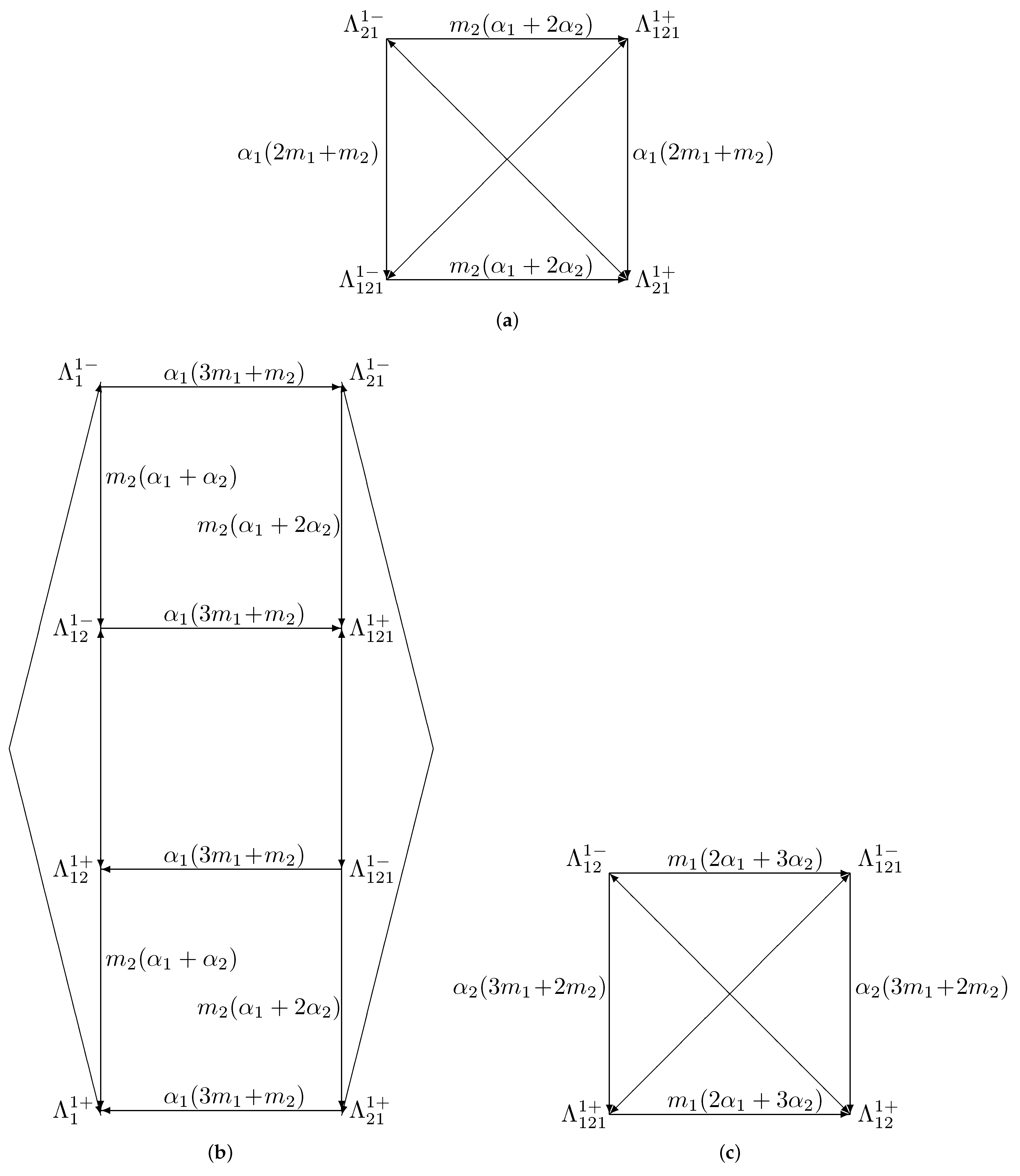
What is peculiar is that the ERs/GVMs of the main multiplet (26) actually consists of three submultiplets with intertwining diagrams as follows:

$$\begin{array}{ccc}& & \begin{array}{ccc}{\mathrm{\Lambda }}_0^{1-}& \genfrac{}{}{0pt}{}{{\mathcal{D}}_{{\alpha }_2}^{m_2}}{⟶}& {\mathrm{\Lambda }}_2^{1-}\\ & & \\ \updownarrow & & \updownarrow \\ & & \\ {\mathrm{\Lambda }}_0^{1+}& \genfrac{}{}{0pt}{}{{\mathcal{D}}_{{\alpha }_2}^{m_2}}{⟵}& {\mathrm{\Lambda }}_2^{1+}\end{array}\mathrm{subtype}\left({\mathrm{A}}_1\right)\hfill \\ & & \phantom{{\mathrm{\Lambda }}_1^{1+}}\hfill \end{array}$$

(27a)

$$\begin{array}{ccc}& & \begin{array}{ccc}{\mathrm{\Lambda }}_1^{1-}& \genfrac{}{}{0pt}{}{{\mathcal{D}}_{{\alpha }_5}^{m_2}}{⟶}& {\mathrm{\Lambda }}_{21}^{1-}\\ & & \\ \updownarrow & & \updownarrow \\ & & \\ {\mathrm{\Lambda }}_1^{1+}& \genfrac{}{}{0pt}{}{{\mathcal{D}}_{{\alpha }_5}^{m_2}}{⟵}& {\mathrm{\Lambda }}_{21}^{1+}\end{array}\mathrm{subtype}\left({\mathrm{B}}_1\right)\hfill \\ & & \phantom{{\mathrm{\Lambda }}_1^{1+}}\hfill \end{array}$$

(27b)

$$\begin{array}{ccc}& & \begin{array}{ccc}{\mathrm{\Lambda }}_{12}^{1-}& \genfrac{}{}{0pt}{}{{\mathcal{D}}_{{\alpha }_6}^{m_2}}{⟶}& {\mathrm{\Lambda }}_{121}^{1+}\\ & & \\ \updownarrow & & \updownarrow \\ & & \\ {\mathrm{\Lambda }}_{12}^{1+}& \genfrac{}{}{0pt}{}{{\mathcal{D}}_{{\alpha }_6}^{m_2}}{⟵}& {\mathrm{\Lambda }}_{121}^{1-}\end{array}\mathrm{subtype}\left({\mathrm{C}}_1\right)\hfill \end{array}$$

(27c)

Next we relax in (26) one of the conditions, namely, we allow $m_1\in IN/2$, still keeping $m_2\in IN$, $m_1\notin IN$. This changes the diagram of subtype ($C_1$), (27c), as given in Figure 2a.

4.2. Main Multiplets When Induction from ${\mathcal{P}}_2$

This case is partly dual to the previous one. When inducing from the maximal parabolic ${\mathcal{P}}_2={\mathcal{M}}_2\oplus {\mathcal{A}}_2\oplus {\mathcal{N}}_2$ there is one ${\mathcal{M}}_2$-compact root, namely, ${\alpha }_2$. We take again the Verma module with ${\mathrm{\Lambda }}_{HC}={\mathrm{\Lambda }}_0^{2-}$. We take ${\chi }_0^{2-}={\chi }_{HC}$. The GVM ${\mathrm{\Lambda }}_0^{2-}$ has one embedded GVM with HW ${\mathrm{\Lambda }}_1^{2-}={\mathrm{\Lambda }}_0^{2-}-m_1{\alpha }_1$, $m_1\in IN$. Altogether, the main multiplet in this case includes the same number of ERs/GVMs as in (17), so we use the same notation only adding super index 2, namely

$$\begin{array}{ccc}\hfill {\chi }_0^{2\pm }& =& \{\mp m_1,\mp m_2;\pm \frac{1}{2}(2m_2+m_1)\}\hfill \\ \hfill {\chi }_2^{2\pm }& =& \{\mp (3m_2+m_1),\pm m_2;\pm \frac{1}{2}(m_2+m_1)\},\hfill \\ \hfill {\chi }_1^{2\pm }& =& \{\pm m_1,\mp (m_2+m_1);\pm \frac{1}{2}(2m_2+m_1)\},\hfill \\ \hfill {\chi }_{12}^{2\pm }& =& \{\mp (3m_2+2m_1),\pm (m_2+m_1);\pm \frac{1}{2}{m}_2\}\hfill \\ \hfill {\chi }_{21}^{2\pm }& =& \{\pm (3m_2+m_1),\mp (2m_2+m_1);\pm \frac{1}{2}(m_2+m_1)\}\hfill \\ \hfill {\chi }_{121}^{2\pm }& =& \{\mp (3m_2+2m_1),\pm (2m_2+m_1);\mp \frac{1}{2}{m}_2\},\hfill \end{array}$$

(28)

In addition, in order to avoid coincidence with (18) we must impose in (28) the conditions: $m_2\notin IN$, $m_2\notin IN/2$, $m_2\notin IN/3$.

Similarly to the ${\mathcal{P}}_1$ case the ERs/GVMs of the main multiplet (28) actually consists of three submultiplets with intertwining diagrams as follows:

$$\begin{array}{ccc}& & \begin{array}{ccc}{\mathrm{\Lambda }}_0^{2-}& \genfrac{}{}{0pt}{}{{\mathcal{D}}_{{\alpha }_1}^{m_1}}{⟶}& {\mathrm{\Lambda }}_1^{2-}\\ & & \\ \updownarrow & & \updownarrow \\ & & \\ {\mathrm{\Lambda }}_0^{2+}& \genfrac{}{}{0pt}{}{{\mathcal{D}}_{{\alpha }_1}^{m_1}}{⟵}& {\mathrm{\Lambda }}_1^{2+}\end{array}\mathrm{subtype}\left({\mathrm{A}}_2\right)\hfill \\ & & \phantom{{\mathrm{\Lambda }}_1^{2+}}\hfill \end{array}$$

(29a)

$$\begin{array}{ccc}& & \begin{array}{ccc}{\mathrm{\Lambda }}_2^{2-}& \genfrac{}{}{0pt}{}{{\mathcal{D}}_{{\alpha }_3}^{m_1}}{⟶}& {\mathrm{\Lambda }}_{12}^{2-}\\ & & \\ \updownarrow & & \updownarrow \\ & & \\ {\mathrm{\Lambda }}_2^{2+}& \genfrac{}{}{0pt}{}{{\mathcal{D}}_{{\alpha }_3}^{m_1}}{⟵}& {\mathrm{\Lambda }}_{12}^{2+}\end{array}\mathrm{subtype}\left({\mathrm{B}}_2\right)\hfill \\ & & \phantom{{\mathrm{\Lambda }}_1^{2+}}\hfill \end{array}$$

(29b)

$$\begin{array}{ccc}& & \begin{array}{ccc}{\mathrm{\Lambda }}_{21}^{2-}& \genfrac{}{}{0pt}{}{{\mathcal{D}}_{{\alpha }_4}^{m_1}}{⟶}& {\mathrm{\Lambda }}_{121}^{2-}\\ & & \\ \updownarrow & & \updownarrow \\ & & \\ {\mathrm{\Lambda }}_{21}^{2+}& \genfrac{}{}{0pt}{}{{\mathcal{D}}_{{\alpha }_4}^{m_1}}{⟵}& {\mathrm{\Lambda }}_{121}^{2+}\end{array}\mathrm{subtype}\left({\mathrm{C}}_2\right)\hfill \end{array}$$

(29c)

Next we relax one of the conditions in (28); namely, we allow $m_2\in IN/2$, still keeping $m_2\notin IN$, $m_2\notin IN/3$. This changes the diagram of subtype ($C_2$), (29c), as given in Figure 2b.

In this case the ER ${\chi }_0^{2+}$ contains a subrepresentation in an infinite-dimensional subspace ${\tilde{\mathcal{D}}}_0^{\prime }$ with conformal weight $d=\frac{3}{2}+c=\frac{3}{2}+m_2+\frac{1}{2}{m}_1=\frac{5}{2},3,\frac{7}{2},\dots .$. It is in the intersection of the images of the operators $G^{+}$ (acting from ${\chi }_0^{2-}$) and ${\mathcal{D}}_{{\alpha }_1}^{m_1}$ (acting from ${\chi }_1^{2+}$).

Next we relax in (28) another condition, namely, we allow $m_2\in IN/3$, still keeping $m_2\notin IN$, $m_2\notin IN/2$. This changes the diagrams of subtypes ($B_1$) and ($C_1$) combining them as given in Figure 2c.

4.3. Reduced Multiplets

There are two reduced multiplets $M_{1k}$, $k=1,2$, which may be obtained by setting the parameter $m_k=0$ when inducing from ${\mathcal{P}}_1$, and two reduced multiplets $M_{2k}$, $k=1,2$, which may be obtained by setting the parameter $m_k=0$ when inducing from ${\mathcal{P}}_2$.

In case $M_{11}$ ($m_1=0$, $m_2\in IN$) the reduced multiplet has six GVMs:

$$\begin{array}{ccc}\hfill {\chi }_0^{1\pm }& =& \{0,\mp m_2;\pm m_2\}={\chi }_1^{1\pm }\hfill \\ \hfill {\chi }_2^{1\pm }& =& \{\mp 3m_2,\pm m_2;\pm \frac{1}{2}{m}_2\}={\chi }_{12}^{1\pm }\hfill \\ \hfill {\chi }_{21}^{1\pm }& =& \{\pm 3m_2,\mp 2m_2;\pm \frac{1}{2}{m}_2\}={\chi }_{121}^{1\pm }\hfill \end{array}$$

(30)

Note that thus reduced multiplet coincides with the reduced multiplet $M_1$ when inducing from the minimal parabolic, cf. (20). The intertwining differential operators are correspondingly given by a recombination of the three submultiplets from (27) and the resulting diagram coincides with the one in (22).

In case $M_{12}$ (when $m_2=0$) the reduced multiplet has six GVMs:

$$\begin{array}{ccc}\hfill {\chi }_0^{1\pm }& =& \{\mp m_1,0;\pm \frac{1}{2}{m}_1\}={\chi }_2^{1\pm }\hfill \\ \hfill {\chi }_1^{1\pm }& =& \{\pm m_1,\mp m_1;\pm \frac{1}{2}{m}_1\}={\chi }_{21}^{1\pm }\hfill \\ \hfill {\chi }_{12}^{1\pm }& =& \{\mp 2m_1,\pm m_1;0\}={\chi }_{121}^{1\mp }\hfill \end{array}$$

(31)

As for the main multiplet, we first consider the subcase $m_1\notin IN$, $m_1\notin IN/2$. Again as in (27) we have three submultiplets; however, the submultiplets $\left(A_1\right)$, $\left(B_1\right)$, $\left(C_1\right)$, are replaced by the KS-related doublets ${\chi }_0^{1\pm }$, ${\chi }_1^{1\pm }$, ${\chi }_{12}^{1\pm }$.

Next we consider the subcase $m_1\notin IN$, $m_1\in IN/2$. As in the first subcase we have the three KS-related doublets, yet for the doublet ${\chi }_{12}^{1\pm }$ the $G^{+}$ KS operator degenerates to the intertwining differential operator ${\mathcal{D}}_{{\alpha }_1}^{2m_1}$, (compare with Figure 2a).

In case $M_{21}$ ($m_1=0$) the reduced multiplet has six GVMs with signatures:

$$\begin{array}{ccc}\hfill {\chi }_0^{2\pm }& =& \{0,\mp m_2;\pm m_2\}={\chi }_1^{2\pm }\hfill \\ \hfill {\chi }_2^{2\pm }& =& \{\mp 3m_2,\pm m_2;\pm \frac{1}{2}{m}_2\}={\chi }_{12}^{2\pm }\hfill \\ \hfill {\chi }_{21}^{2\pm }& =& \{\pm 3m_2,\mp 2m_2;\pm \frac{1}{2}{m}_2\}={\chi }_{121}^{2\mp }\hfill \end{array}$$

(32)

As for the main multiplet, we first consider the subcase $m_2\notin IN$, $m_2\notin IN/2$, $m_2\notin IN/3$. Again as in (27) we have three submultiplets, however the submultiplets $\left(A_2\right)$, $\left(B_2\right)$, $\left(C_2\right)$, are replaced by the KS-related doublets ${\chi }_0^{2\pm }$, ${\chi }_2^{2\pm }$, ${\chi }_{21}^{2\pm }$.

Next we consider the subcase $m_2\notin IN$, $m_2\in IN/2$, $m_2\notin IN/3$. As in the first subcase we have the three KS-related doublets, yet for the doublet ${\chi }_{21}^{2\pm }$ the $G^{+}$ KS operator degenerates to the intertwining differential operator ${\mathcal{D}}_{{\alpha }_2}^{2m_2}$, compare with Figure 2c.

The ER ${\chi }_0^{2+}$ contains a subrepresentation in an infinite-dimensional subspace ${\tilde{\mathcal{D}}}_1^{\prime }$ with conformal weight $d=\frac{3}{2}+c=\frac{3}{2}+m_2=2,3,4,\dots$. It is the image of the KS operator $G^{+}$ (acting from ${\chi }_0^{2-}$).

Next we consider the subcase $m_2\notin IN$, $m_2\notin IN/2$, $m_2\in IN/3$. As for the main multiplet the submultiplets corresponding to $\left(B_2\right)$, $\left(C_2\right)$ are combined. Here the result is a quartet (compare with Figure 2c):

$$\begin{array}{ccc}{\chi }_2^{2-}& \genfrac{}{}{0pt}{}{{\mathcal{D}}_{{\alpha }_1}^{3m_2}}{⟶}& {\chi }_{21}^{2-}\\ & & \\ \updownarrow & & \updownarrow \\ & & \\ {\chi }_2^{2+}& \genfrac{}{}{0pt}{}{{\mathcal{D}}_{{\alpha }_1}^{3m_2}}{⟵}& {\chi }_{21}^{2+}\end{array}$$

(33)

In case $M_{22}$ ($m_2=0$, $m_1\in IN$) the reduced multiplet has six GVMs with signatures:

$$\begin{array}{ccc}\hfill {\chi }_0^{2\pm }& =& \{\mp m_1,0;\pm \frac{1}{2}{m}_1\}={\chi }_2^{2\pm }\hfill \\ \hfill {\chi }_1^{2\pm }& =& \{\pm m_1,\mp m_1;\pm \frac{1}{2}{m}_1\}={\chi }_{21}^{2\pm }\hfill \\ \hfill {\chi }_{12}^{2\pm }& =& \{\mp 2m_1,\pm m_1;0\}={\chi }_{121}^{2\pm }\hfill \end{array}$$

(34)

Note that thus reduced multiplet coincides with the reduced multiplet $M_2$ when inducing from the minimal parabolic, cf. (23). The intertwining differential operators are correspondingly given by a recombination of the three submultiplets from (29) and the resulting diagram coincides with the one in (24).

References

- Dobrev, V.K. Invariant Differential Operators for Non-Compact Lie Groups: Parabolic Subalgebras. Rev. Math. Phys. 2008, 20, 407–449. [Google Scholar] [CrossRef] [Green Version]
- Vladimir, D. Invariant Differential Operators, Volume 1: Non-Compact Semisimple Lie Algebras and Groups; De Gruyter Studies in Mathematical Physics; De Gruyter: Berlin, Germany; Boston, MA, USA, 2016; Volume 35, ISBN 978-3-1142764-6. [Google Scholar]
- Dobrev, V.K. Invariant Differential Operators for Non-Compact Lie Algebras Parabolically Related to Conformal Lie Algebras. J. High Energy Phys. 2013, 2, 015. [Google Scholar] [CrossRef] [Green Version]
- Dobrev, V.K. Multiplet Classification of Reducible Verma Modules over the G2 Algebra. J. Phys. Conf. Ser. 2019, 1194, 012027. [Google Scholar] [CrossRef]
- Langlands, R.P. On the Classification of Irreducible Representations of Real Algebraic Groups; Math. Surveys and Monographs, first as IAS Princeton preprint 1973; AMS: Providence, RI, USA, 1988; Volume 31.
- Zhelobenko, D.P. Harmonic Analysis on Semisimple Complex Lie Groups; Nauka: Moscow, Russia, 1974. (In Russian) [Google Scholar]
- Knapp, A.W.; Zuckerman, G.J. Classification Theorems for Representations of Semisimple Groups; Lecture Notes in Math.; Springer: Berlin, Germany, 1977; Volume 587, pp. 138–159. [Google Scholar]
- Dobrev, V.K.; Mack, G.; Petkova, V.B.; Petrova, S.G.; Todorov, I.T. Harmonic Analysis on the n-Dimensional Lorentz Group and Its Applications to Conformal Quantum Field Theory; Lecture Notes in Physics; Springer: Berlin, Germany, 1977; Volume 63. [Google Scholar]
- Knapp, A.W. Representation Theory of Semisimple Groups (An Overview Based on Examples); Princeton University Press: Princeton, NJ, USA, 1986. [Google Scholar]
- Harish-Chandra. Representations of a semi-simple Lie group on a Banach space I. Trans. Amer. Math. Soc. 1953, 75, 185, Erratum in 1954, 76, 236; Amer. J. Math. 1955, 77, 734; Erratum in 1956, 78, 564. [Google Scholar] [CrossRef]
- Dobrev, V.K. Canonical Construction of Intertwining Differential Operators Associated with Representations of Real Semisimple Lie Groups. Rept. Math. Phys. 1988, 25, 159–181. [Google Scholar] [CrossRef]
- Dobrev, V.K. Multiplet classification of the reducible elementary representations of real semi-simple Lie groups: The SOep,q example. Lett. Math. Phys. 1985, 9, 205–211. [Google Scholar] [CrossRef]
- Bernstein, I.N.; Gel’fand, I.M.; Gel’fand, S.I. Structure of representations generated by highest weight vectors. Funkts. Anal. Prilozh. 1971, 5, 1–9, Erratum in Funct. Anal. Appl. 1971, 5, 1–8. [Google Scholar] [CrossRef]
- Dixmier, J. Enveloping Algebras; North Holland: New York, NY, USA, 1977. [Google Scholar]
- Vogan, D.A., Jr. The unitary dual of G2. Inv. Math. 1994, 116, 677–791. [Google Scholar] [CrossRef]
- Knapp, A.W.; Stein, E.M. Intertwining operators for semisimple groups. Ann. Math. 1980, 93, 489–578, Erratum in Inv. Math. 1980, 60, 9–84. [Google Scholar] [CrossRef]
- Harish-Chandra. Discrete series for semisimple Lie groups: I-II. Ann. Math. 1965, 113, 241–318, Erratum in 1966, 116, 1–111. [Google Scholar]
Figure 1.
Main multiplets for using induction from the minimal parabolic.
Figure 2.
(a) Submultiplets type () for using induction from the maximal parabolic for , , , , the (anti)diagonal arrows represent the KS operators; (b) Submultiplets type ()+() for using induction from the maximal parabolic for , , , , the up-down arrows represent four pairs of KS operators; (c) Submultiplets type () for using induction from the maximal parabolic for , , , the (anti)diagonal arrows represent the KS operators.
Publisher’s Note: MDPI stays neutral with regard to jurisdictional claims in published maps and institutional affiliations. |
© 2022 by the author. Licensee MDPI, Basel, Switzerland. This article is an open access article distributed under the terms and conditions of the Creative Commons Attribution (CC BY) license (https://creativecommons.org/licenses/by/4.0/).
Share and Cite
MDPI and ACS Style
Dobrev, V.K. Heisenberg Parabolic Subgroups of Exceptional Non-Compact G2(2) and Invariant Differential Operators. Symmetry 2022, 14, 660. https://doi.org/10.3390/sym14040660
AMA Style
Dobrev VK. Heisenberg Parabolic Subgroups of Exceptional Non-Compact G2(2) and Invariant Differential Operators. Symmetry. 2022; 14(4):660. https://doi.org/10.3390/sym14040660
Chicago/Turabian StyleDobrev, V.K. 2022. "Heisenberg Parabolic Subgroups of Exceptional Non-Compact G2(2) and Invariant Differential Operators" Symmetry 14, no. 4: 660. https://doi.org/10.3390/sym14040660
Note that from the first issue of 2016, this journal uses article numbers instead of page numbers. See further details here.