Figure 1.
Trajectory of the spacecraft escaping from the Earth [
1].
Figure 1.
Trajectory of the spacecraft escaping from the Earth [
1].
Figure 2.
Switching function and thrust control versus transfer time.
Figure 2.
Switching function and thrust control versus transfer time.
Figure 3.
Movement of charged particles due to the interaction with the Earth’s magnetic field [
8].
Figure 3.
Movement of charged particles due to the interaction with the Earth’s magnetic field [
8].
Figure 4.
Coordinates for a point in space, given by B and L or R and .
Figure 4.
Coordinates for a point in space, given by B and L or R and .
Figure 5.
Example of a model for the Van Allen Belts; axes x and y are measured in Earth radii, 6378 km [
9].
Figure 5.
Example of a model for the Van Allen Belts; axes x and y are measured in Earth radii, 6378 km [
9].
Figure 8.
Maximum and minimum inclination of the lunar orbit with respect to the Earth’s celestial equator .
Figure 8.
Maximum and minimum inclination of the lunar orbit with respect to the Earth’s celestial equator .
Figure 9.
Neural network with two hidden layers of 10 neurons.
Figure 9.
Neural network with two hidden layers of 10 neurons.
Figure 10.
Use of successive swing-bys with the moon in the ISEE-3/ICE comet mission [
23].
Figure 10.
Use of successive swing-bys with the moon in the ISEE-3/ICE comet mission [
23].
Figure 11.
Particle fluence as a function of mission time for the five initial eccentricities chosen (0; 0.2; 0.4; 0.6; 0.8) and considering the NEXT propulsion system ( mN and s), km and .
Figure 11.
Particle fluence as a function of mission time for the five initial eccentricities chosen (0; 0.2; 0.4; 0.6; 0.8) and considering the NEXT propulsion system ( mN and s), km and .
Figure 12.
Particle fluence as a function of mission time for the four chosen propulsion systems—NEXT, ionic, BHT-8000 and PPS-1500—and considering an initial orbit with km, and .
Figure 12.
Particle fluence as a function of mission time for the four chosen propulsion systems—NEXT, ionic, BHT-8000 and PPS-1500—and considering an initial orbit with km, and .
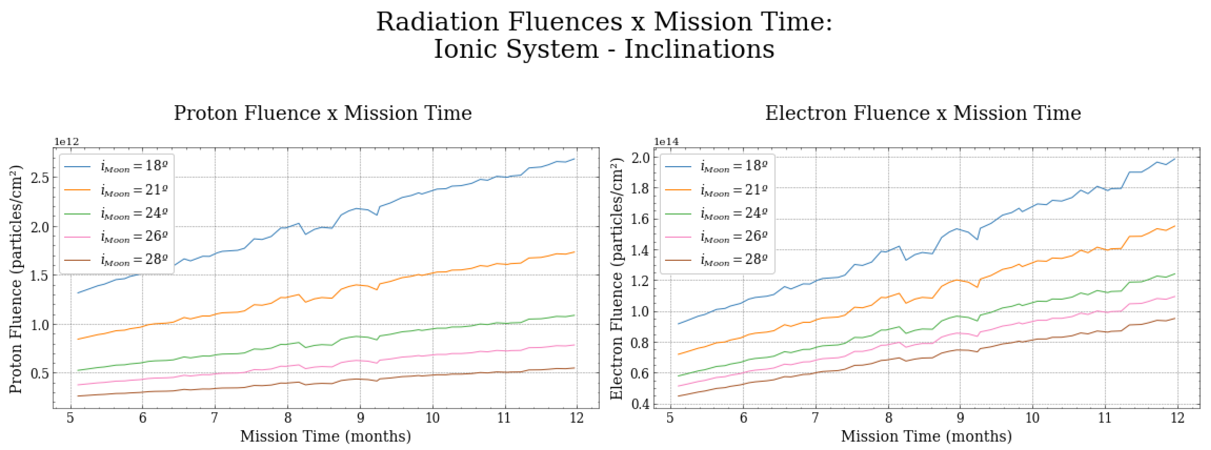
Figure 13.
Particle fluence as a function of total mission time for the five chosen lunar inclinations (), considering a propulsion system NEXT, km and .
Figure 13.
Particle fluence as a function of total mission time for the five chosen lunar inclinations (), considering a propulsion system NEXT, km and .
Figure 14.
Particle fluence as a function of mission time for the two initial perigee heights chosen ( km and km) and considering the propulsion system NEXT ( mN and s), with and .
Figure 14.
Particle fluence as a function of mission time for the two initial perigee heights chosen ( km and km) and considering the propulsion system NEXT ( mN and s), with and .
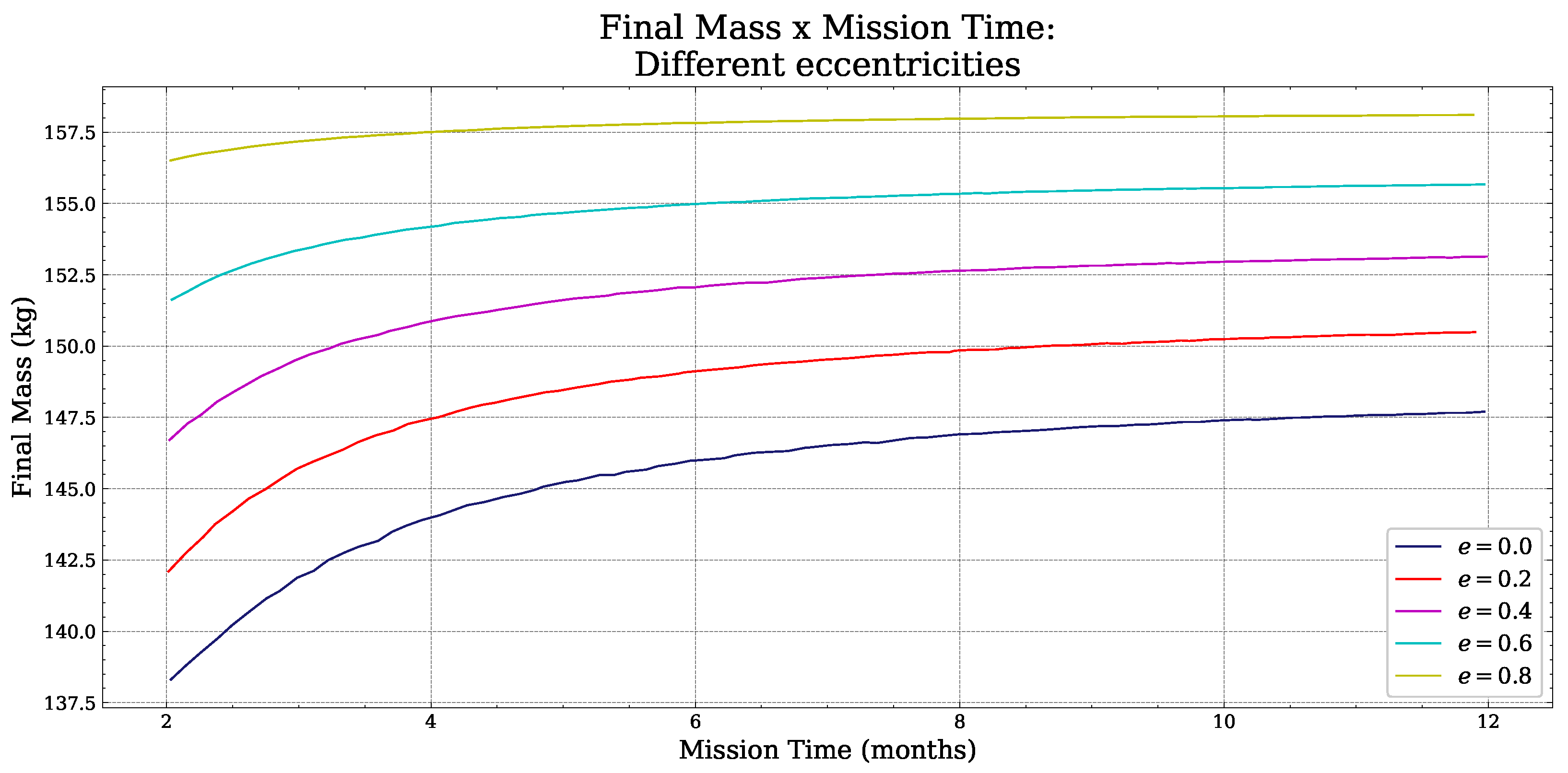
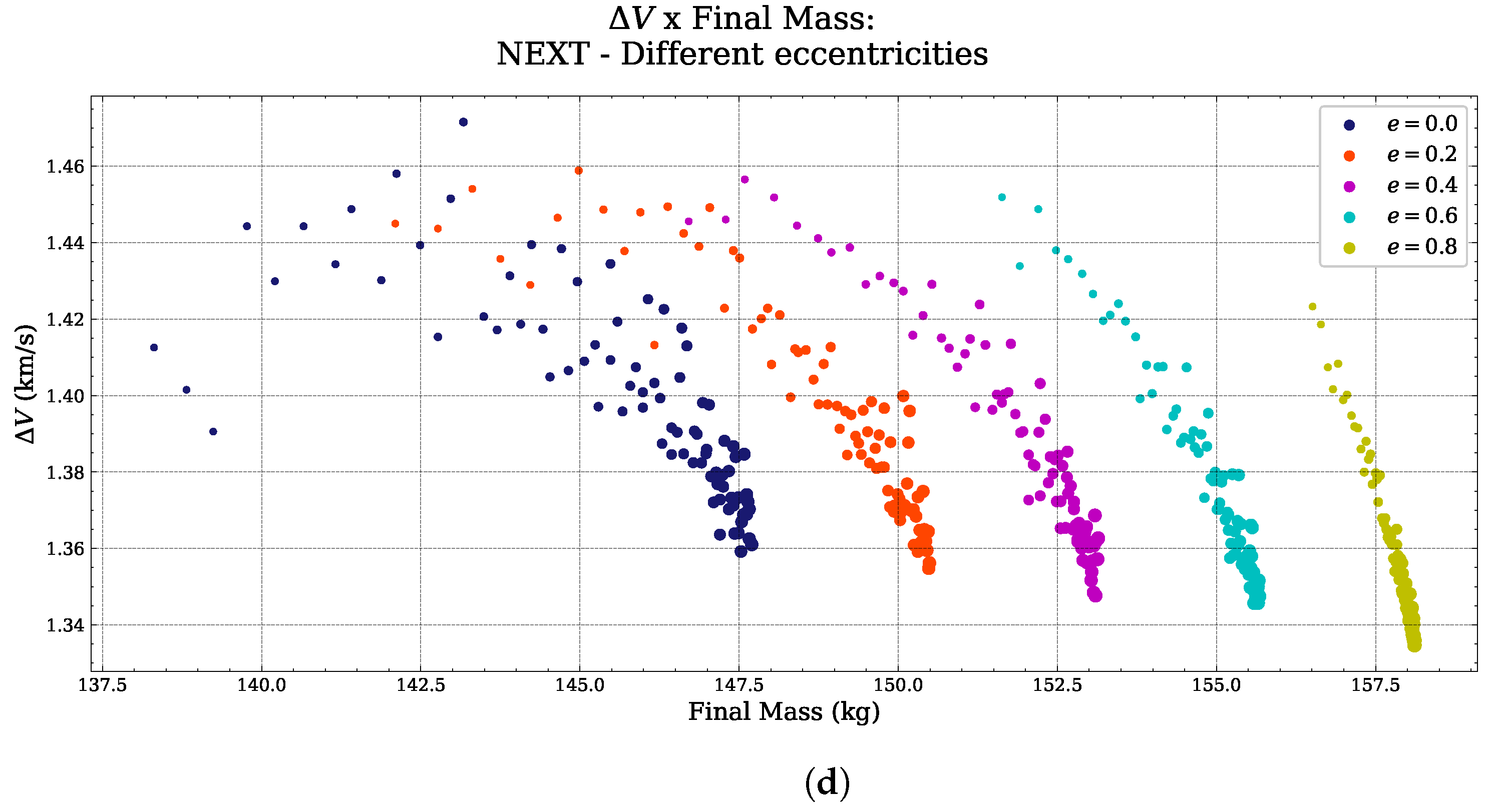
Figure 15.
Final mass as a function of mission time for the five initial eccentricities chosen (0; 0.2; 0.4; 0.6; 0.8) and considering the system of propulsion NEXT ( mN and s), km and .
Figure 15.
Final mass as a function of mission time for the five initial eccentricities chosen (0; 0.2; 0.4; 0.6; 0.8) and considering the system of propulsion NEXT ( mN and s), km and .
Figure 16.
Final mass as a function of mission time for the four chosen propulsion systems—NEXT, Ionic, BHT-8000 and PPS-1500—and considering an initial orbit with km, and .
Figure 16.
Final mass as a function of mission time for the four chosen propulsion systems—NEXT, Ionic, BHT-8000 and PPS-1500—and considering an initial orbit with km, and .
Figure 17.
Final mass as a function of mission time for the two initial perigee heights chosen ( km and km) and considering the NEXT propulsion system ( mN and s), with and .
Figure 17.
Final mass as a function of mission time for the two initial perigee heights chosen ( km and km) and considering the NEXT propulsion system ( mN and s), with and .
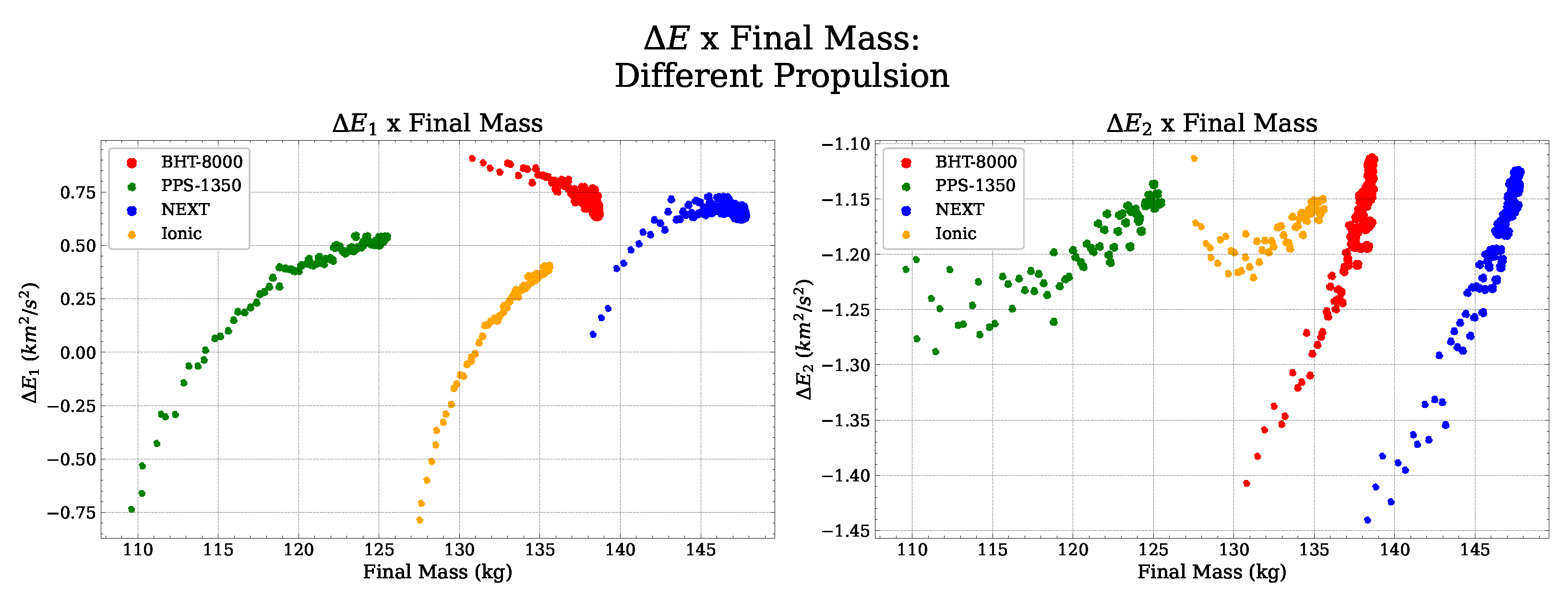
Figure 18.
Energy gain, in its two configurations, as a function of mission time for the four chosen propulsion systems—ionic, NEXT, BHT-8000 and PPS-1500—and considering an initial orbit with km, , and a moon approach distance km.
Figure 18.
Energy gain, in its two configurations, as a function of mission time for the four chosen propulsion systems—ionic, NEXT, BHT-8000 and PPS-1500—and considering an initial orbit with km, , and a moon approach distance km.
Figure 19.
Energy gain, in its two configurations, as a function of mission time for the five initial eccentricities chosen (0; 0.2; 0.4; 0.6; 0.8), km, and km. (a) Ionic propulsion system. (b) PPS-1350 propulsion system. (c) NEXT propulsion system. (d) BHT-8000 propulsion system.
Figure 19.
Energy gain, in its two configurations, as a function of mission time for the five initial eccentricities chosen (0; 0.2; 0.4; 0.6; 0.8), km, and km. (a) Ionic propulsion system. (b) PPS-1350 propulsion system. (c) NEXT propulsion system. (d) BHT-8000 propulsion system.
Figure 20.
Energy gain, in its two configurations, as a function of mission time for the two chosen initial perigee heights ( km and km) and considering the ionic propulsion system, with , and km.
Figure 20.
Energy gain, in its two configurations, as a function of mission time for the two chosen initial perigee heights ( km and km) and considering the ionic propulsion system, with , and km.
Figure 21.
Energy gain, in its two configurations, as a function of mission time for the five approach distances chosen initials (1910.7; 2084.4; 2258.1; 2431.8; 2605.5 km) and considering the ionic propulsion system, km, km, .
Figure 21.
Energy gain, in its two configurations, as a function of mission time for the five approach distances chosen initials (1910.7; 2084.4; 2258.1; 2431.8; 2605.5 km) and considering the ionic propulsion system, km, km, .
Figure 22.
Speed gain as a function of mission time for the four chosen propulsion systems—ionic, NEXT, BHT-8000 and PPS-1500—and considering the initial parameters as: km, , and km.
Figure 22.
Speed gain as a function of mission time for the four chosen propulsion systems—ionic, NEXT, BHT-8000 and PPS-1500—and considering the initial parameters as: km, , and km.
Figure 23.
Speed gain as a function of mission time for the five initial eccentricities chosen (0; 0.2; 0.4; 0.6; 0.8), km, and km. (a) Ionic propulsion system. (b) BHT-8000 propulsion system. (c) NEXT propulsion system. (d) PPS-1350 propulsion system.
Figure 23.
Speed gain as a function of mission time for the five initial eccentricities chosen (0; 0.2; 0.4; 0.6; 0.8), km, and km. (a) Ionic propulsion system. (b) BHT-8000 propulsion system. (c) NEXT propulsion system. (d) PPS-1350 propulsion system.
Figure 24.
Speed gain as a function of mission time for the two initial perigee heights chosen ( km and km) and considering the ionic propulsion system, with , and km.
Figure 24.
Speed gain as a function of mission time for the two initial perigee heights chosen ( km and km) and considering the ionic propulsion system, with , and km.
Figure 25.
Speed gain as a function of mission time for the five initial chosen approach distances (1910.7; 2084.4; 2258.1; 2431.8; 2605.5 km) and considering the ionic propulsion system, km, km, .
Figure 25.
Speed gain as a function of mission time for the five initial chosen approach distances (1910.7; 2084.4; 2258.1; 2431.8; 2605.5 km) and considering the ionic propulsion system, km, km, .
Figure 26.
Energy gain, in its two configurations, as a function of the final mass, where the size of the dots represents the electron fluence, for the four chosen propulsion systems—ionic, NEXT, BHT-8000 and PPS-1500—and considering an initial orbit with km, , and moon approach distance km.
Figure 26.
Energy gain, in its two configurations, as a function of the final mass, where the size of the dots represents the electron fluence, for the four chosen propulsion systems—ionic, NEXT, BHT-8000 and PPS-1500—and considering an initial orbit with km, , and moon approach distance km.
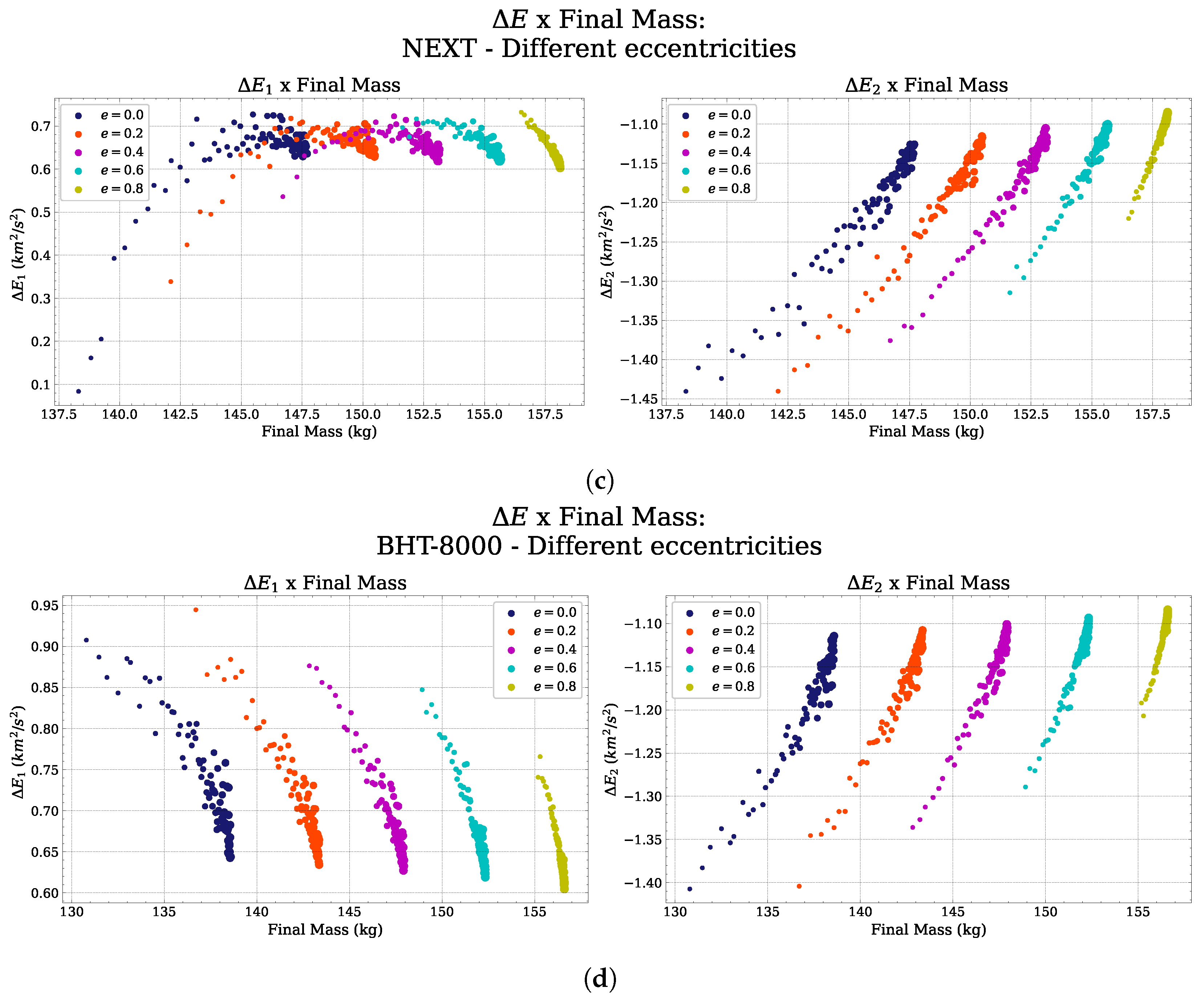
Figure 27.
Energy gain, in its two configurations, as a function of final mass for the five initial eccentricities chosen (0; 0.2; 0.4; 0.6; 0.8), km, and km. (a) Ionic propulsion system. (b) PPS-1350 propulsion system. (c) NEXT propulsion system. (d) BHT-8000 propulsion system.
Figure 27.
Energy gain, in its two configurations, as a function of final mass for the five initial eccentricities chosen (0; 0.2; 0.4; 0.6; 0.8), km, and km. (a) Ionic propulsion system. (b) PPS-1350 propulsion system. (c) NEXT propulsion system. (d) BHT-8000 propulsion system.
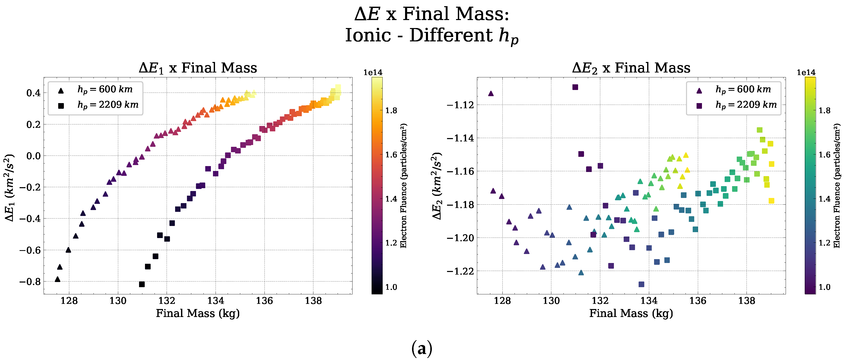
Figure 28.
Energy gain, in its two configurations, as a function of the final mass, where the color of the dots represents the fluence of electrons, for the two initial perigee heights chosen ( km and km), with , and km. (a) Ionic propulsion system. (b) PPS-1350 propulsion system. (c) BHT-8000 propulsion system. (d) NEXT propulsion system.
Figure 29.
Energy gain, in its two configurations, as a function of the final mass for the five approximation distances chosen initials (1910.7; 2084.4; 2258.1; 2431.8; 2605.5 km) and considering the ionic propulsion system, km, km, .
Figure 29.
Energy gain, in its two configurations, as a function of the final mass for the five approximation distances chosen initials (1910.7; 2084.4; 2258.1; 2431.8; 2605.5 km) and considering the ionic propulsion system, km, km, .
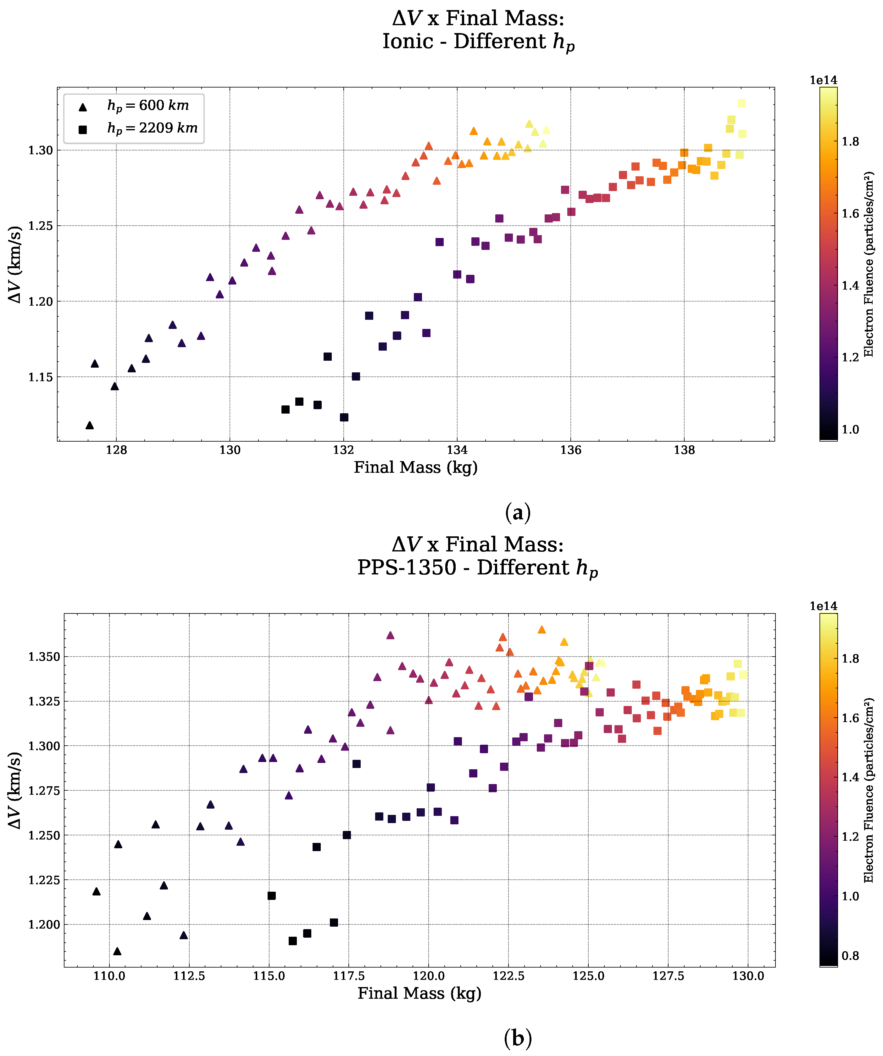
Figure 30.
Velocity gain as a function of final mass, where the size of the dots represents the fluence of electrons, for the four chosen propulsion systems—ionic, NEXT, BHT-8000 and PPS-1500—and considering the initial parameters as: km, , and km.
Figure 30.
Velocity gain as a function of final mass, where the size of the dots represents the fluence of electrons, for the four chosen propulsion systems—ionic, NEXT, BHT-8000 and PPS-1500—and considering the initial parameters as: km, , and km.
Figure 31.
Gain in velocity as a function of final mass, where the size of the dots represents the fluence of electrons, for the five initial eccentricities chosen (0; 0.2; 0.4; 0.6; 0.75), km, and km. (a) Ionic propulsion system. (b) PPS-1350 propulsion system. (c) BHT-8000 propulsion system. (d) NEXT propulsion system.
Figure 32.
Gain in velocity as a function of the final mass, where the color of the dots represents the fluence of electrons, for the two initial perigee heights chosen ( km and km), with , and km. (a) Ionic propulsion system. (b) PPS-1350 propulsion system. (c) BHT-8000 propulsion system. (d) NEXT propulsion system.
Figure 33.
Speed gain as a function of final mass for the five initial chosen approximation distances (1910.7; 2084.4; 2258.1; 2431.8; 2605.5 km) and considering the ionic propulsion system, km, km, .
Figure 33.
Speed gain as a function of final mass for the five initial chosen approximation distances (1910.7; 2084.4; 2258.1; 2431.8; 2605.5 km) and considering the ionic propulsion system, km, km, .
Figure 34.
Model and data comparison for the electron fluences.
Figure 34.
Model and data comparison for the electron fluences.
Figure 35.
Model and data comparison for the proton fluences.
Figure 35.
Model and data comparison for the proton fluences.
Table 1.
Regression statistics for electron fluence, first considering all parameters and then excluding the final mass and mission time.
Table 1.
Regression statistics for electron fluence, first considering all parameters and then excluding the final mass and mission time.
| Regression Statistic | 7 Parameters | 5 Parameters |
|---|
| Multiple R | 0.90 | 0.86 |
| R-squared | 0.81 | 0.75 |
| R-square adjusted | 0.80 | 0.75 |
| Standard error | 2.9 × | 3.3 × |
| Observation count | 928 | 928 |
Table 2.
ANOVA for electron fluence.
Table 2.
ANOVA for electron fluence.
| | gl | SQ | MQ | F | p-Value |
|---|
| Regression | 7 | 3.2 × | 4.6 × | 545.0 | 0 |
| Residual | 920 | 7.7 × | 8.4 × | | |
| Total | 927 | 4.0 × | | | |
Table 3.
Regression coefficients for the electron fluence.
Table 3.
Regression coefficients for the electron fluence.
| | Coefficient | Standard Error | t-Statistic | p-Value |
|---|
| Intersection | 5.6 × | 3.7 × | 15.4 | 1.3 × |
| (mN) | 1.0 × | 2.3 × | 4.5 | 6.4 × |
| (s) | −1.6 × | 3.5 × | −4.6 | 5.5 × |
| (km) | −1.3 × | 1.4 × | −9.4 | 5.8 × |
| e | −2.0 × | 2.5 × | −8.3 | 5.3 × |
(degrees) | −1.2 × | 3.2 × | −36.8 | 2.6 × |
| t (months) | 6.5 × | 1.1 × | 5.8 | 7.0 × |
| m (kg) | 1.0 × | 7.6 × | 1.3 | 1.9 × |
Table 4.
Regression statistics for proton fluence, first considering all parameters and then excluding the final mass and mission time.
Table 4.
Regression statistics for proton fluence, first considering all parameters and then excluding the final mass and mission time.
| Regression Statistic | 7 Parameters | 5 Parameters |
|---|
| Multiple R | 0.92 | 0.82 |
| R-squared | 0.84 | 0.68 |
| R-square adjusted | 0.84 | 0.67 |
| Standard error | 1.6 × | 2.2 × |
| Observation count | 928 | 928 |
Table 5.
ANOVA for proton fluence.
Table 5.
ANOVA for proton fluence.
| | gl | SQ | MQ | F | p-Value |
|---|
| Regression | 7.00 | 1.2 × | 1.7 × | 697.8 | 0 |
| Residual | 920.00 | 2.3 × | 2.5 × | | |
| Total | 927.00 | 1.4 × | | | |
Table 6.
Regression coefficients for the proton fluence.
Table 6.
Regression coefficients for the proton fluence.
| | Coefficient | Standard Error | t-Statistic | p-Value |
|---|
| Intersection | 2.0 × | 2.0 × | 10.0 | 2.7 × |
| (mN) | 8.1 × | 1.2 × | 6.6 | 9.2 × |
| (s) | −1.3 × | 1.9 × | −6.6 | 5.4 × |
| (km) | −9.3 × | 7.7 × | −12.1 | 2.2 × |
| e | −1.7 × | 1.3 × | −12.6 | 1.2 × |
(degrees) | −3.8 × | 1.7 × | −21.7 | 6.3 × |
| t (months) | 5.6 × | 6.0 × | 9.3 | 1.0 × |
| m (kg) | 1.8 × | 4.1 × | 4.2 | 2.4 × |
Table 7.
Scaler and model comparison for three regression methods. It is clear that the linear regression was improved by the use of non-linear ML models.
Table 7.
Scaler and model comparison for three regression methods. It is clear that the linear regression was improved by the use of non-linear ML models.
| Scaler | Method | R-Square | MSE |
|---|
| MinMax | Linear Regression | 0.815 | 0.0086 |
| MinMax | Support Vector Machine | 0.931 | 0.0032 |
| MinMax | Neural Network | 0.962 | 0.0018 |
| Standard | Linear Regression | 0.815 | 0.0086 |
| Standard | Support Vector Machine | 0.926 | 0.0034 |
| Standard | Neural Network | 0.977 | 0.0011 |
Table 8.
Summary of the improvements made in the ANN model.
Table 8.
Summary of the improvements made in the ANN model.
| Improvement | R-Squared | MSE |
|---|
| None | 0.875 | 0.0058 |
| Pipeline | 0.966 | 0.0016 |
| Scaling | 0.977 | 0.0011 |
| Hyperparameter Optimization | 0.997 | 0.0002 |


