Least-Squares Finite Element Method for Solving Stokes Flow under Point Source Magnetic Field

Abstract

The least-squares finite element method (LSFEM) is successfully employed for the discretization of the Stokes equations and the numerical computation of the behaviour of two-dimensional Stokes flow in a straight rectangular channel under the effect of a point-source magnetic field. LSFEM has several advantages in terms of theory and computing, where it can always create a symmetric, positive-definite algebraic system of equations. It also allows for using an equal order shape function for both velocity and pressure, and it is not required to satisfy the Ladyzhenskaya–Babuška–Brezzi (LBB) condition. Despite this, LSFEM has an issue where low-order nodal expansions tend to lock. Thus, the present study proposes the discretization of the problem domain using higher-order nodes elements with full numerical integration. Results concerning velocity contour and streamlines pattern are shown. On the basis of current findings, it can be concluded that the LSFEM can be used to solve Stokes flow problem under the point source magnetic field.

1. Introduction

Stokes flow is incompressible viscous flow in slow motion. Stokes flow has numerous crucial functions in industries such as medical applications, the design of innovative materials, lab-on-chip technologies, microdevices, and biological systems. For instance, dust settles, and microbes swim in a fluid, both of which are instances of Stokes flow. Stokes flow is also known as the flow of high-viscosity fluids, such as melt extrusion or the transportation of paints, heavy oils, or food-processing ingredients [1]. Some essential characteristics of Stokes flow, such as negligibility of inertial forces, reversibility, and the minimal energy dissipation theorem, were explored by [2]. Navier–Stokes flow situations can be subdivided into Stokes flow problems, with nonlinear convective components being very minor or ignored [1]. The authors in [1] presented two cases, steady-state Stokes flow ($Re=0$) and a very low Reynolds number Stokes flow problem solved with Navier–Stokes equation ($Re=1$). As a problem model, they utilized a square cavity with a moving top lid with constant velocity, and solved this problem using the dual reciprocity boundary element method (DRBEM). Then, they came up with an iterative DRBEM for solving the Stokes flow problem by adding another model problem, a circular cavity [3]. In the study by [4], the two-dimensional Stokes flow problem was solved by developing the analytical method of superposition. A rectangular chamber containing a cylinder was utilised as a model problem to investigate distributive mixing processes in periodic Stokes flows. The authors in [5] used vorticity–velocity formulation in combination with the multiquadric method (MQ) to handle steady-state Stokes flow problems in 2D and 3D. Three numerical problems were used to evaluate the truth and effectiveness of the MQ scheme: a 2D square cavity problem, a 3D cubic cavity flow problem, and a circular cavity. The 2D Stokes flows in a lid-driven square cavity, rectangle cavity with wave-shaped bottom, and cubic cavity were solved using the method of fundamental solutions (MFS) by [6].

The interaction of fluid in motion with a magnetic effect is among the most studied due to its many industrial and medical applications. Magnetic devices for cell separation, targeted medication delivery, magnetic cancer tumour therapy, bleeding reduction during surgery, and magnetic tracers are just a few of the uses for magnets being developed [7,8,9,10]. Thus, the present study investigates Stokes flow with the effect of a point-source magnetic field. Ferrohydrodynamics (FHD) and magnetohydrodynamics (MHD) are a branch of fluid mechanics. The body force in FHD is due to polarisation force, while the Lorentz force occurs in MHD when an electric current passes through a fluid and exerts an effect on it [11]. The 2D MHD Stokes flow produced by a concentrated point force was analytically obtained by [12]. The 2D MHD Stokes flow equations in a lid-driven cavity and a backward-facing step channel subjected to the external magnetic effect with different directions were solved by [13] using the radial basis function (RBF) approximation method. The authors in [14] employed RBF for solving 2D MHD Stokes flow in a square constricted enclosure with a moving left wall with enforced magnetic field in the direction. Then, they solved MHD Stokes flow using the same numerical method in the same problem domain, but the external magnetic field from three different directions was applied [15]. The authors in [16] studied Stokes flow in a lid-driven and circular cavity under an external magnetic field source. Fluid flow equations in their problem were comparable to those used in FHD. They implemented DRBEM in solving this problem. In [17], the solution of the MHD Stokes eigenvalue problem was approximated by using the Chebyshev spectral collocation method (CSCM).

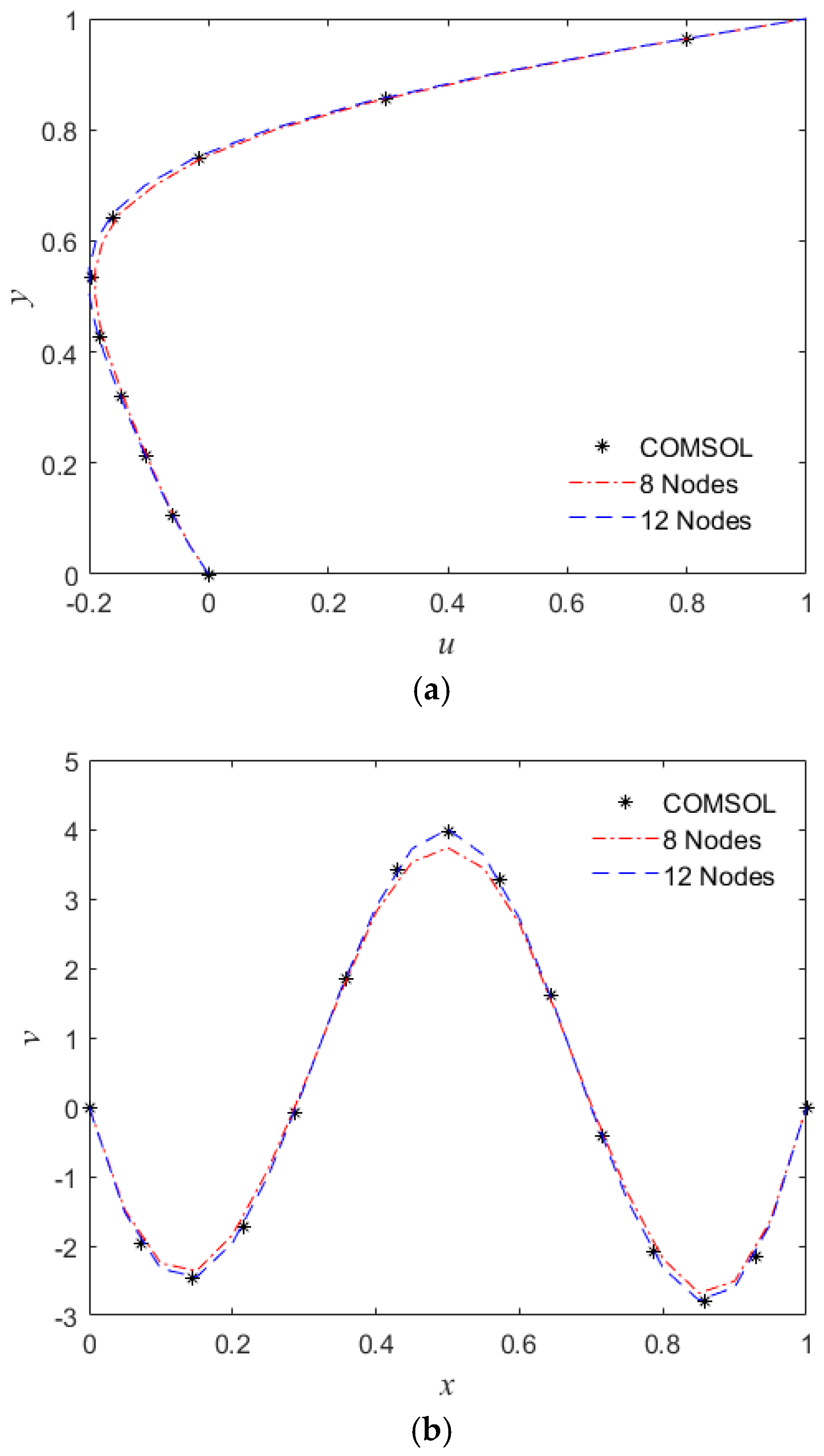
In this study, the least-squares finite element method (LSFEM) was employed to solve two-dimensional Stokes flow subjected to point magnetic source. The authors in [18] studied the theory of LSFEM for the numerical solution of elliptic boundary-value problems. The use of LSFEM in solving the Stokes problem was first presented by [19]. They developed LSFEM on the basis of first-order velocity–pressure–vorticity formulation for a simple one-dimensional Stokes problem. On the basis of their findings, LSFEM leads to a minimisation problem rather than to a saddle-point problem, which happened in the Galerkin mixed method. Thus, LSFEM does not depend on the LBB condition. LSFEM has an additional vorticity degree of freedom as compared to the mixed FEM, which only has pressure and velocity. This makes the LSFEM matrix larger than the mixed FEM, and it theoretically takes a longer time to solve. However, the matrix generated by LSFEM is symmetric and positive-definite, whereas the matrix generated by mixed FEM is not symmetric due to the convective term, and the matrix is a zero diagonal because of the absence of a pressure term in the continuity equation. As such, mixed FEM requires a direct solver with pivoting. On the other hand, LSFEM can be solved by using a very efficient iterative solver such as preconditioned conjugate gradient method in a fully parallel environment. This offers the method additional advantages from a computational point of view. The benefit of using the LSFEM over other vorticity-related techniques is that no artificial numerical boundary conditions for the vorticity must be created [20,21,22,23,24]. The authors in [25] presented LSFEM for Navier–Stokes equations of viscous incompressible fluids. They focused on first-order systems based on velocity–vorticity formulation associated with the mixed formulation. Predominantly low-order nodal expansion was employed to develop the discrete finite element model in the context of least-squares finite element formulations. However, low order nodal expansions tend to lock when the least-squares functional is a nonequivalent formulation. Locking occurs in lower-order elements because the element’s kinematics are insufficient to represent the correct solution. It means the effect of a reduced rate of convergence in dependence of a parameter. Therefore, the present study is proposed to use the higher-order element to prevent this locking issue.

In this paper, a fully developed, steady, laminar, electrically nonconducting, incompressible fluid was considered under the influence of an external point-source magnetic field. This study proposes LSFEM for solving Stokes flow subjected to a point-source magnetic field in a straight rectangular channel problem. This serves as a fundamental work to investigate and overcome the issue in LSFEM in the presence of highly nonlinear body force. Results concerning velocity contour and streamline patterns are presented and discussed. To the authors’ knowledge, this study is the first implementation of the LSFEM for the study of Stokes flow under a point-source magnetic field.

2. Mathematical Formulation

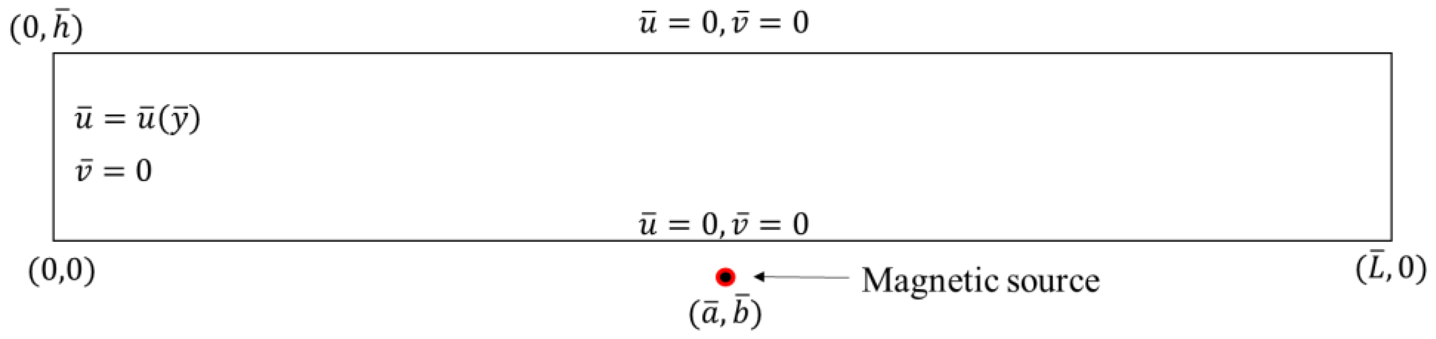
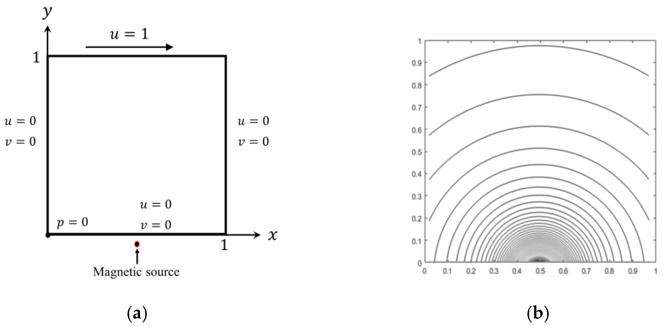
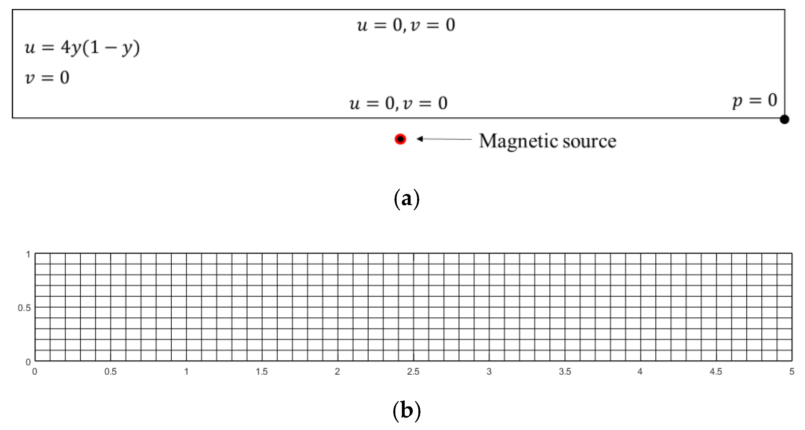
Flow was considered to be fully developed, incompressible, steady, laminar, and electrically nonconducting under the point-source magnetic field. The fluid was flowing through two parallel plates (channel). The length of the plates was $\overline{L}$ and the distance between them was $\overline{h}$, such that $\overline{L}/\overline{h}=5$. The entrance velocity was assumed to be fully developed flow, whereas the Neumann boundary condition for the exit velocity was set as zero. A no-slip condition was imposed on the upper and bottom walls of the channel, and a zero-pressure boundary was imposed at the right lower corner of the channel. The magnetic source was located below the bottom wall of the channel, as shown in Figure 1.

The governing equations of the fluid flow are similar to those derived for ferrohydrodynamics (FHD) [11,16]. Continuity and momentum equations defining the two-dimensional flow are given by

$$\frac{\partial \overline{u}}{\partial \overline{x}}+\frac{\partial \overline{v}}{\partial \overline{y}}=0,$$

(1)

$$\overline{\rho }\left(\overline{u}\frac{\partial \overline{u}}{\partial \overline{x}}+\overline{v}\frac{\partial \overline{u}}{\partial \overline{y}}\right)=-\frac{\partial \overline{p}}{\partial \overline{x}}+\overline{\mu }\left(\frac{{\partial }^2\overline{u}}{\partial {\overline{x}}^2}+\frac{{\partial }^2\overline{u}}{\partial {\overline{y}}^2}\right)+{\overline{\mu }}_0\overline{M}\frac{\partial \overline{H}}{\partial \overline{x}},$$

(2)

$$\overline{\rho }\left(\overline{u}\frac{\partial \overline{v}}{\partial \overline{x}}+\overline{v}\frac{\partial \overline{v}}{\partial \overline{y}}\right)=-\frac{\partial \overline{p}}{\partial \overline{y}}+\overline{\mu }\left(\frac{{\partial }^2\overline{v}}{\partial {\overline{x}}^2}+\frac{{\partial }^2\overline{v}}{\partial {\overline{y}}^2}\right)+{\overline{\mu }}_0\overline{M}\frac{\partial \overline{H}}{\partial \overline{y}}.$$

(3)

The boundary conditions of the problem are summarised as follows:

$$\begin{array}{ll}\mathrm{Inflow} & \left(\overline{x}=0,0\le \overline{y}\le \overline{h}\right):\overline{u}=\overline{u}\left(\overline{y}\right),\overline{v}=0,\\ \mathrm{Outflow} & \left(\overline{x}=\overline{L},0\le \overline{y}\le \overline{h}\right):\partial \left(\overline{R}\right)/\partial \overline{x},\\ \mathrm{Upper} \mathrm{wall} & \left(\overline{y}=\overline{h},0\le \overline{x}\le \overline{L}\right):\overline{u}=0,\overline{v}=0\\ \mathrm{Lower} \mathrm{wall} & \left(\overline{y}=0,0\le \overline{x}\le \overline{L}\right):\overline{u}=0,\overline{v}=0\end{array}\}$$

(4)

where $\overline{u}\left(\overline{y}\right)$ is a parabolic velocity profile corresponding to fully developed flow, $\overline{R}$ stands for $\overline{u}$ or $\overline{v}$, $\overline{\rho }$ is the fluid density, $\overline{\mu }$ is the dynamic viscosity, and ${\overline{\mu }}_0$ is the magnetic permeability of the fluid; $\overline{H}$ is magnetic field intensity, and $\overline{M}$ is magnetisation. Terms ${\mu }_0\overline{M}\partial \overline{H}/\partial \overline{x}$ and ${\mu }_0\overline{M}\partial \overline{H}/\partial \overline{y}$ from (2) and (3) represent the magnetisation force per unit volume and are known as the FHD terms.

According to FHD, magnetisation property $\overline{M}$ is generally a function of magnetic field intensity, fluid temperature, and density of fluid. Since temperature was considered to be negligible in this present study, the following relation for magnetic fluid was considered:

$$\overline{M}=\chi \overline{H}$$

(5)

where $\chi$ is magnetic susceptibility.

The components of magnetic field intensity ${\overline{H}}_x$ and ${\overline{H}}_y$ along the $\overline{x}$ and $\overline{y}$ directions are given as

$${\overline{H}}_x=\frac{\gamma }{2\pi }\frac{\overline{x}-\overline{a}}{{\left(\overline{x}-\overline{a}\right)}^2+{\left(\overline{y}-\overline{b}\right)}^2},$$

(6)

$${\overline{H}}_y=-\frac{\gamma }{2\pi }\frac{\overline{y}-\overline{b}}{{\left(\overline{x}-\overline{a}\right)}^2+{\left(\overline{y}-\overline{b}\right)}^2},$$

(7)

where $(\overline{a},\overline{b})$ is the point where the magnetic source is placed, and $\gamma$ is the magnetic field strength at the point. Magnitude $\overline{H}$ of the magnetic field intensity is given by

$$\overline{H}={\left[{\overline{H}}_x{}^2+{\overline{H}}_y{}^2\right]}^{\frac{1}{2}}=\frac{\gamma }{2\pi }\frac{1}{\sqrt{{\left(\overline{x}-\overline{a}\right)}^2+{\left(\overline{y}-\overline{b}\right)}^2}}.$$

(8)

Dimensionless Form

Equations (1)–(3) and (8) could be nondimensionalised by using the following nondimensional variables:

$$x=\frac{\overline{x}}{\overline{h}},y=\frac{\overline{y}}{\overline{h}},u=\frac{\overline{u}}{{\overline{u}}_r},v=\frac{\overline{v}}{{\overline{u}}_r},p=\frac{\overline{p}}{\overline{\rho }{\overline{u}}_r{}^2},H=\frac{\overline{H}}{{\overline{H}}_0}$$

(9)

where ${\overline{H}}_0$ is magnetic field intensity, $\overline{h}$ is the height between two plates, and ${\overline{u}}_r$ is the maximal velocity at entrance.

First, dimensionless variables are rearranged and then substituted into Equations (1)–(3). The dimensionless form of the governing equations of the fluid flow under the effect of the point source magnetic field are obtained as

$$\frac{\partial u}{\partial x}+\frac{\partial v}{\partial y}=0,$$

(10)

$$Re\left(u\frac{\partial u}{\partial x}+v\frac{\partial u}{\partial y}\right)=-\frac{\partial p}{\partial x}+\left(\frac{{\partial }^{2}u}{\partial x^2}+\frac{{\partial }^{2}u}{\partial y^2}\right)+\frac{Mn}{Re}H\frac{\partial H}{\partial x},$$

(11)

$$Re\left(u\frac{\partial v}{\partial x}+v\frac{\partial v}{\partial y}\right)=-\frac{\partial p}{\partial y}+\left(\frac{{\partial }^{2}v}{\partial x^2}+\frac{{\partial }^{2}v}{\partial y^2}\right)+\frac{Mn}{Re}H\frac{\partial H}{\partial y}.$$

(12)

The dimensionless forms of the boundary conditions are given by

$$\begin{array}{ll}\mathrm{Inflow} & \left(x=0,0\le y\le 1\right):u=4y\left(1-y\right),v=0\\ \mathrm{Outflow} & \left(x=5,0\le y\le h\right):\partial u/\partial x=0,\partial v/\partial x=0\\ \mathrm{Upper} \mathrm{wall} & \left(y=1,0\le x\le 5\right):u=0,v=0\\ \mathrm{Lower} \mathrm{wall} & \left(y=0,0\le x\le 5\right):u=0,v=0\end{array}\}$$

(13)

The nondimensional parameters are defined as

$$Re=\frac{\overline{h}\overline{\rho }{\overline{u}}_r}{\overline{\mu }}, Mn=\frac{{\overline{\mu }}_0\chi {\overline{H}}_0{}^2}{\overline{\rho }{\overline{u}}_r{}^2},$$

(14)

where $Re$ is the Reynolds number, and $Mn$ is the magnetic number. The magnitude $\overline{H}$ of magnetic field intensity in the dimensionless form obtained by substituting the dimensional variables into (8):

$$H=\frac{\left|b\right|}{\sqrt{{\left(x-a\right)}^2+{\left(y-b\right)}^2}}.$$

(15)

We aimed to investigate Stokes flow under the effect of a point-source magnetic field. Hence, for the Stokes flow case, low Reynolds number $(Re\ll 1)$ was considered, and convection terms in (11) and (12) were neglected. Then, the governing equations for the Stokes flow were written as follows

$$\frac{\partial u}{\partial x}+\frac{\partial v}{\partial y}=0,$$

(16)

$$\frac{{\partial }^{2}u}{\partial x^2}+\frac{{\partial }^{2}u}{\partial y^2}=\frac{\partial p}{\partial x}-MH\frac{\partial H}{\partial x},$$

(17)

$$\frac{{\partial }^{2}v}{\partial x^2}+\frac{{\partial }^{2}v}{\partial y^2}=\frac{\partial p}{\partial y}-MH\frac{\partial H}{\partial y},$$

(18)

where $M=Mn/Re$.

3. Least-Squares Finite Element Model

In this section, the least-squares formulation for the Stokes equations is presented. This study focuses on first-order systems based on the velocity–vorticity formulation associated with the mixed formulation.

3.1. Stokes First-Order System

Two-dimensional, laminar, steady, incompressible, electrically nonconducting fluid was considered under the effect of a point-source magnetic field. The governing equations for Stokes flow subjected to a point-source magnetic field in the dimensionless form are written in Equations (16)–(18).

The following vorticity function is introduced:

$$w=\frac{\partial v}{\partial x}-\frac{\partial u}{\partial y}.$$

(19)

The vorticity-based equivalent first-order system is given by

$$\frac{\partial u}{\partial x}+\frac{\partial v}{\partial y}=0,$$

(20)

$$\frac{\partial p}{\partial x}+\frac{\partial w}{\partial y}=MH\frac{\partial H}{\partial x},$$

(21)

$$\frac{\partial p}{\partial y}-\frac{\partial w}{\partial x}=MH\frac{\partial H}{\partial y},$$

(22)

$$w+\frac{\partial u}{\partial y}-\frac{\partial v}{\partial x}=0.$$

(23)

3.2. Least-Squares Formulation

For the two-dimensional case represented by system Equations (20)–(23), least-squares functional $I^e$ over a typical element ${\Omega }^e$ takes the form

$$I^e=\frac{1}{2}{\displaystyle \underset{{\Omega }^e}{\int }\left(R_1^2+R_2^2+R_3^2+R_4^2\right)} dxdy,$$

(24)

where

$$R_1=\frac{\partial p}{\partial x}+\frac{\partial w}{\partial y}-MH\frac{\partial H}{\partial x},$$

$$R_2=\frac{\partial p}{\partial y}-\frac{\partial w}{\partial x}-MH\frac{\partial H}{\partial y},$$

$$R_3=w+\frac{\partial u}{\partial y}-\frac{\partial v}{\partial x},$$

$$R_4=\frac{\partial u}{\partial x}+\frac{\partial v}{\partial y}.$$

(25)

3.3. Finite Element Model

Variables of problem $(u,v,p,w)$ are approximated by expansions of the form

$$u(x,y)={\displaystyle \sum _{i=1}^m{N}_i(x,y)u_i} , v(x,y)={\displaystyle \sum _{i=1}^m{N}_i(x,y)v_i},$$

$$p(x,y)={\displaystyle \sum _{i=1}^m{N}_i(x,y)p_i} , w(x,y)={\displaystyle \sum _{i=1}^m{N}_i(x,y)w_i},$$

(26)

where $N_i$ is the serendipity interpolation functions, and $(u_i,v_i,p_i,w_i)$ are nodal values of $(u,v,p,w)$. Then, the expressions form in (26) is used to approximated the dependent variables in (23). Equation (25) becomes

$$R_1=\frac{\partial N_i{p}_i}{\partial x}+\frac{\partial N_i{w}_i}{\partial y}-MH\frac{\partial H}{\partial x},$$

$$R_2=\frac{\partial N_i{p}_i}{\partial y}-\frac{\partial N_i{w}_i}{\partial x}-MH\frac{\partial H}{\partial y},$$

$$R_3=N_i{w}_i+\frac{\partial N_i{u}_i}{\partial y}-\frac{\partial N_i{v}_i}{\partial x},$$

$$R_4=\frac{\partial N_i{u}_i}{\partial x}+\frac{\partial N_i{v}_i}{\partial y}.$$

(27)

Equation (27) is expanded; then, (24) yields

$$\begin{array}{cc}{I}^e\hfill & =\frac{1}{2}{\displaystyle \underset{{\Omega }^e}{\int }\left(R_1^2+R_2^2+R_3^2+R_4^2\right)} dxdy\hfill \\ & =\frac{1}{2}{\displaystyle {\int }_{{\Omega }^e}[p_i^2{\left(\frac{\partial N_i}{\partial x}\right)}^2+2p_i{w}_i\left(\frac{\partial N_i}{\partial x}\right)\left(\frac{\partial N_i}{\partial y}\right)-2p_{i}MH\frac{\partial H}{\partial x}\frac{\partial N_i}{\partial x}}\hfill \\ & +w_i^2{\left(\frac{\partial N_i}{\partial y}\right)}^2-2w_{i}MH\frac{\partial H}{\partial x}\left(\frac{\partial N_i}{\partial y}\right)+{\left(MH\frac{\partial H}{\partial x}\right)}^2+p_i^2{\left(\frac{\partial N_i}{\partial y}\right)}^2\hfill \\ & -2p_i{w}_i\left(\frac{\partial N_i}{\partial y}\right)\left(\frac{\partial N_i}{\partial x}\right)-2p_{i}MH\frac{\partial H}{\partial y}\frac{\partial N_i}{\partial y}+w_i{}^2{\left(\frac{\partial N_i}{\partial x}\right)}^2\hfill \\ & +2w_{i}MH\frac{\partial H}{\partial y}\left(\frac{\partial N_i}{\partial x}\right)+{\left(MH\frac{\partial H}{\partial y}\right)}^2+{\left(N_i{w}_i\right)}^2+2N_i{w}_i{u}_i\left(\frac{\partial N_i}{\partial y}\right)\hfill \\ & -2N_i{w}_i{v}_i\left(\frac{\partial N_i}{\partial x}\right)+u_i^2{\left(\frac{\partial N_i}{\partial y}\right)}^2-2u_i{v}_i\left(\frac{\partial N_i}{\partial y}\right)\left(\frac{\partial N_i}{\partial x}\right)+v_i^2{\left(\frac{\partial N_i}{\partial x}\right)}^2\hfill \\ & +u_i^2{\left(\frac{\partial N_i}{\partial x}\right)}^2+v_i^2{\left(\frac{\partial N_i}{\partial y}\right)}^2+2u_i{v}_i\left(\frac{\partial N_i}{\partial x}\right)\left(\frac{\partial N_i}{\partial y}\right)]dxdy.\hfill \end{array}$$

(28)

Minimising the least-squares functional in (24) for nodal values of velocities, pressure, and vorticity obtains

$$\partial I^e=\frac{\partial I^e}{\partial u_i}\delta u_i+\frac{\partial I^e}{\partial v_i}\delta v_i+\frac{\partial I^e}{\partial p_i}\delta p_i+\frac{\partial I^e}{\partial w_i}\delta w_i=0,$$

which yields four sets of $m$ equations each over a typical element:

$$\frac{\partial I^e}{\partial u_i}=0,\frac{\partial I^e}{\partial v_i}=0,\frac{\partial I^e}{\partial p_i}=0,\frac{\partial I^e}{\partial w_i}=0,$$

(29)

for $i=1,2,\dots m,$, where

$$\begin{gathered} \frac{\partial I^e}{\partial u_i}={\displaystyle \underset{{\Omega }^e}{\int }[u_i\left(\frac{\partial N_i}{\partial y}\right)\left(\frac{\partial N_i}{\partial y}\right)+u_i\left(\frac{\partial N_i}{\partial x}\right)\left(\frac{\partial N_i}{\partial x}\right)-v_i\left(\frac{\partial N_i}{\partial y}\right)\left(\frac{\partial N_i}{\partial x}\right)} \\ +v_i\left(\frac{\partial N_i}{\partial x}\right)\left(\frac{\partial N_i}{\partial y}\right)+N_i{w}_i\left(\frac{\partial N_i}{\partial y}\right)]dxdy=0, \end{gathered}$$

$$\begin{gathered} \frac{\partial I^e}{\partial v_i}={\displaystyle \underset{{\Omega }^e}{\int }[v_i\left(\frac{\partial N_i}{\partial x}\right)\left(\frac{\partial N_i}{\partial x}\right)+v_i\left(\frac{\partial N_i}{\partial y}\right)\left(\frac{\partial N_i}{\partial y}\right)-u_i\left(\frac{\partial N_i}{\partial x}\right)\left(\frac{\partial N_i}{\partial y}\right)} \\ +u_i\left(\frac{\partial N_i}{\partial y}\right)\left(\frac{\partial N_i}{\partial x}\right)-N_i{w}_i\left(\frac{\partial N_i}{\partial x}\right)]dxdy=0, \end{gathered}$$

$$\begin{gathered} \frac{\partial I^e}{\partial p_i}={\displaystyle \underset{{\Omega }^e}{\int }[\left(\frac{\partial N_i}{\partial x}\right)\left(\frac{\partial N_i}{\partial x}\right)+p_i\left(\frac{\partial N_i}{\partial y}\right)\left(\frac{\partial N_i}{\partial y}\right)+w_i\left(\frac{\partial N_i}{\partial x}\right)\left(\frac{\partial N_i}{\partial y}\right)} \\ -w_i\left(\frac{\partial N_i}{\partial y}\right)\left(\frac{\partial N_i}{\partial x}\right)-MH\frac{\partial H}{\partial x}\frac{\partial N_i}{\partial x}-MH\frac{\partial H}{\partial y}\frac{\partial N_i}{\partial y}]dxdy=0, \end{gathered}$$

$$\begin{gathered} \frac{\partial I^e}{\partial w_i}={\displaystyle \underset{{\Omega }^e}{\int }[N_i{u}_i\frac{\partial N_i}{\partial y}-N_i{v}_i\frac{\partial N_i}{\partial x}+w_i\left(\frac{\partial N_i}{\partial y}\right)\left(\frac{\partial N_i}{\partial y}\right)} \\ +w_i\left(\frac{\partial N_i}{\partial x}\right)\left(\frac{\partial N_i}{\partial x}\right)+N_i^2{w}_i-MH\frac{\partial H}{\partial x}\left(\frac{\partial N_i}{\partial y}\right)+MH\frac{\partial H}{\partial y}\left(\frac{\partial N_i}{\partial x}\right)]dxdy=0. \end{gathered}$$

The resulting finite element equations are given in matrix form as follows:

$$\left[\begin{array}{cccc}\left[S_{ij}{}^{11}+S_{ij}{}^{22}\right]& \left[S_{ij}{}^{12}-S_{ij}{}^{21}\right]& \left[0\right]& \left[S_{ij}{}^{20}\right]\\ \left[S_{ij}{}^{21}-S_{ij}{}^{12}\right]& \left[S_{ij}{}^{11}+S_{ij}{}^{22}\right]& \left[0\right]& -\left[S_{ij}{}^{10}\right]\\ \left[0\right]& \left[0\right]& \left[S_{ij}{}^{11}+S_{ij}{}^{22}\right]& \left[S_{ij}{}^{12}-S_{ij}{}^{21}\right]\\ \left[S_{ij}{}^{02}\right]& -\left[S_{ij}{}^{01}\right]& \left[S_{ij}{}^{21}-S_{ij}{}^{12}\right]& \left[S_{ij}{}^{11}+S_{ij}{}^{22}\right]+\left[S_{ij}{}^{00}\right]\end{array}\right]\left\{\begin{array}{c}{u}_i\\ v_i\\ p_i\\ w_i\end{array}\right\}=\left[\begin{array}{c}{F}_i{}^1\\ F_i{}^2\\ F_i{}^3\\ F_i{}^4\end{array}\right]$$

(30)

where coefficient matrices are defined by

$$\begin{array}{c}{S}_{ij}^{00}={\displaystyle {\int }_{{\Omega }^e}{N}_i{N}_j dxdy},S_{ij}^{01}={\displaystyle {\int }_{{\Omega }^e}{N}_i\frac{\partial N_j}{\partial x} dxdy},S_{ij}^{02}={\displaystyle {\int }_{{\Omega }^e}{N}_i\frac{\partial N_j}{\partial y} dxdy},\hfill \\ S_{ij}^{10}={\displaystyle {\int }_{{\Omega }^e}\frac{\partial N_i}{\partial x}{N}_j dxdy},S_{ij}^{20}={\displaystyle {\int }_{{\Omega }^e}\frac{\partial N_i}{\partial y}{N}_j dxdy},S_{ij}^{11}={\displaystyle {\int }_{{\Omega }^e}\frac{\partial N_i}{\partial x}\frac{\partial N_j}{\partial x} dxdy},\hfill \\ S_{ij}^{22}={\displaystyle {\int }_{{\Omega }^e}\frac{\partial N_i}{\partial y}\frac{\partial N_j}{\partial y} dxdy},S_{ij}^{12}={\displaystyle {\int }_{{\Omega }^e}\frac{\partial N_i}{\partial x}\frac{\partial N_j}{\partial y} dxdy},S_{ij}^{21}={\displaystyle {\int }_{{\Omega }^e}\frac{\partial N_i}{\partial y}\frac{\partial N_j}{\partial x} dxdy},\hfill \end{array}$$

$$\begin{gathered} F_i^1={\displaystyle {\int }_{{\Omega }^e}0 dxdy},F_i^2={\displaystyle {\int }_{{\Omega }^e}0 dxdy},F_i^3={\displaystyle {\int }_{{\Omega }^e}\left(\frac{\partial N_i}{\partial x}MH\frac{\partial H}{\partial x}+\frac{\partial N_i}{\partial y}MH\frac{\partial H}{\partial y}\right)} dxdy, \\ {F}_i^4={\displaystyle {\int }_{{\Omega }^e}\left(\frac{\partial N_i}{\partial y}MH\frac{\partial H}{\partial x}-\frac{\partial N_i}{\partial x}MH\frac{\partial H}{\partial y}\right)} dxdy. \end{gathered}$$

The Gaussian quadrature is applied to integrate a function over a rectangular master element ${\overline{\Omega }}_R$. The Gaussian quadrature over a function in a normalised coordinate $(\xi ,\eta )$ can be expressed as

$$\begin{gathered} {\displaystyle {\int }_{{\overline{\Omega }}_R}F}(\xi ,\eta ) d\xi d\eta ={\displaystyle {\int }_{-1}^1\left[{\displaystyle {\int }_{-1}^{1}F(\xi ,\eta )d\eta }\right]} d\xi \approx {\displaystyle {\int }_{-1}^1\left[{\displaystyle \sum _{J=1}^{N}F({\xi }_i,{\eta }_j)w_j}\right]} d\xi \\ \approx {\displaystyle \sum _{i=1}^M{\displaystyle \sum _{j=1}^{N}F({\xi }_i,{\eta }_j)w_i{w}_j}}, \end{gathered}$$

(31)

where $M$ and $N$ are the number of quadrature points in the $\xi$ and $\eta$ directions, respectively, $({\xi }_i,{\eta }_j)$ is Gaussian points, and $w_i$ and $w_j$ denote the corresponding Gaussian weight. The number of Gaussian points was selected on the basis of the largest-degree polynomial when the integrand was of different degrees in $\xi$ and $\eta$. In most cases, interpolation functions are of the same degree in both $\xi$ and $\eta$; thus, $M=N$.

3.4. Solution of Linear Equation

Stokes governing equations only have the linear term in the momentum equation; thus, they are easier to solve compared to governing equations that have nonlinear terms. The system of governing equations can be written in matrix form as

$$[K(U)]U=\left\{F\right\},$$

(32)

where $K$ is the stiffness matrix, $U$ represents the vector of the degree of freedom, and $F$ is the force vector. The Gaussian elimination method is used to solve the linear equations. For the system in (32), this algorithm is given by

$$K\left(U^i\right)U^{i+1}=F\left(U^i\right),$$

(33)

where superscripts $i$ indicate the iteration number. Then, the solution can be calculated by

$$U^{i+1}={\left[K\left(U^i\right)\right]}^{-1}F\left(U^i\right).$$

(34)

4. MATLAB Code Validation

MATLAB was used to create the least-squares formulation source code. The source code was checked for reliability and appropriate operation using a benchmark problem. The lid-driven cavity problem was selected as a benchmark in this work since it is a common benchmark for verifying stable Stokes equations.

4.1. Stokes Flow without Magnetic Effect

The domain of the problem was discretized into the uniform rectangular element as shown in Figure 2a, while the boundary conditions are shown in Figure 2b. The top lid moved with a horizontal velocity of $u=1$ in the positive x-direction, and a no-slip condition was imposed on the remaining walls. Pressure was applied on the bottom left corner of the cavity. The solution of the system was computed for comparison with the literature.

The mesh shown in Figure 2a was generated using Gmsh, which is external software that can easily create geometries, mesh, and element nodes. This software can directly export the mesh to MATLAB software using a postprocessor. Hence, Gmsh is an alternative tool in creating meshing, and can help to simplify the work in MATLAB.

The first verification of the Stokes flow problem against the benchmark problem was computed using a low-order node number, a 4-node rectangular element. The computed components of velocity along horizontal and vertical lines through the central cavity were compared with the study by [26].

The comparison for the different node rectangular element in LSFEM and [26] is shown in Figure 3. The results for the LSFEM using a 4-node element were inaccurate when compared with [26]. This proves that low-order nodes in LSFEM have a lock issue, as stated in [25]. This means that the accuracy of the solution tended to lock if we attempted to refine the meshing. Then, we computed the solution of the problem using higher-order rectangular element nodes, namely, 8 and 12-node. Results from the LSFEM for 8 and 12 nodes agreed well with those computed by [26].

4.2. Stokes Flow with Magnetic Effect

The source code of Stokes flow subjected to the point-source magnetic field problem was also validated with the simulation obtained from COMSOL Multiphysics 5.2. The problem domain and boundary conditions are shown in Figure 4. The magnetic source was located very close to the bottom of the cavity and below.

For Stokes flow under the effect of the point-source magnetic field, the magnetic number was set to be $M=\mathrm{10,000}$. Results of the present study were compared with those of COMSOL Multiphysics software 5.2, and are shown in Figure 5. Figure 5 shows that there was a slight difference between the 8 and 12-node serendipity element. However, the 12-node element showed excellent agreement with COMSOL compared to the 8-node element.

Results of the streamline pattern are demonstrated in Figure 6 to compare the 12-node element with COMSOL Multiphysics. The streamline that was formed from this source code had a similar pattern to that of COMSOL Multiphysics. Hence, to solve the locking problem of a low-order nodal in LSFEM, a 12-node serendipity element was used here for solving the Stokes flow under the point magnetic source.

5. Results and Discussion

Two-dimensional Stokes flow in a straight rectangular channel subjected to a point-source magnetic field was solved by using LSFEM. The same assumption as in the previous simulation prevailed, where it was assumed that the Stokes flow was fully developed, steady, laminar, incompressible, electrically nonconducting, and under the effect of the point-source magnetic field. In this channel, a spatially varying magnetic field was generated by placing the magnetic source below the lower wall of the channel at the location $(x,y)=(2.5,-0.2)$. Different magnetic numbers $M (150, 250, 350, 600)$ were studied. From the simulation, the flow characteristics are discussed.

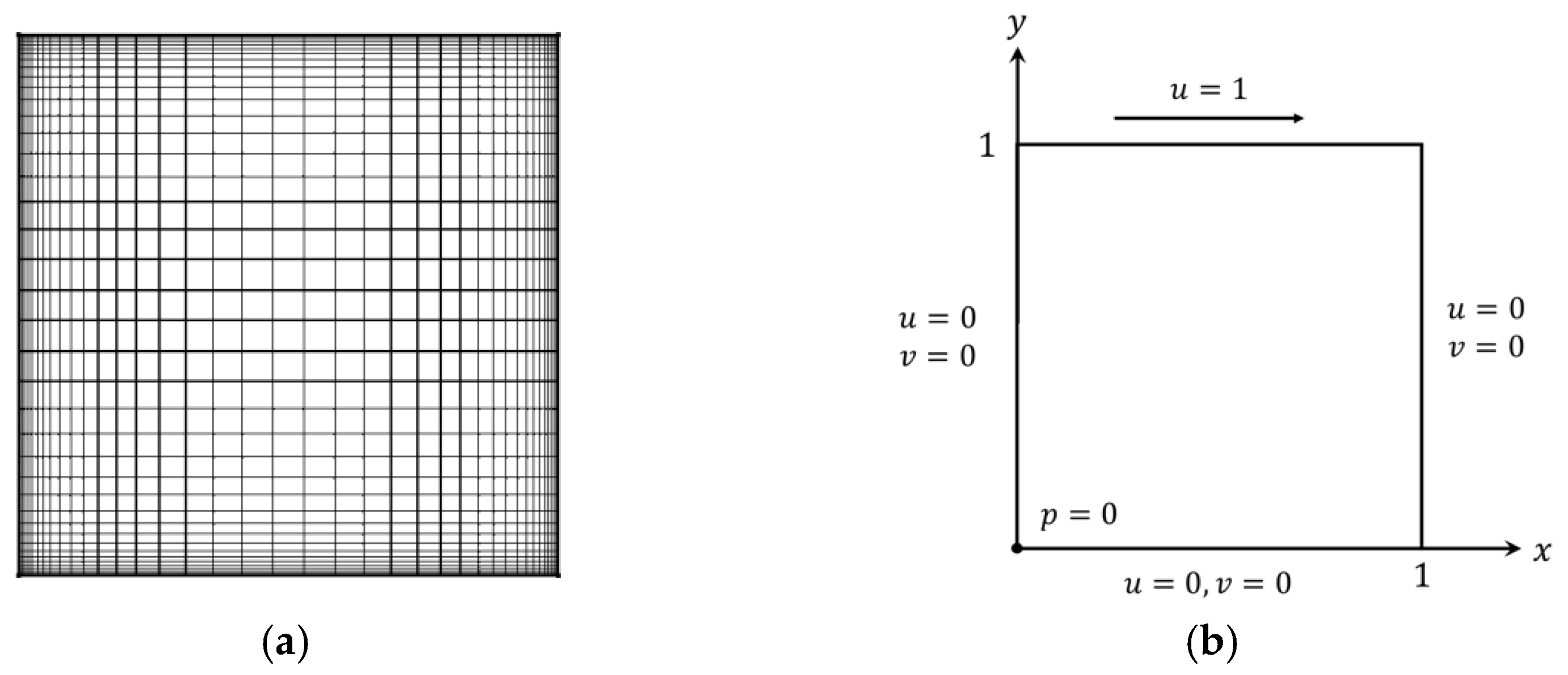
Figure 7a displays the computational domain and boundary conditions. Entrance velocity was assumed to be a fully developed flow, whereas the Neumann boundary condition for the exit velocity was set as zero. A no-slip condition was imposed on the upper and bottom walls of the channel, and a zero-pressure boundary is imposed at the lower right corner of the channel. The mesh for the computational domain is shown in Figure 7b. Structured rectangular mesh with a 12-node serendipity element was used for the computational domain.

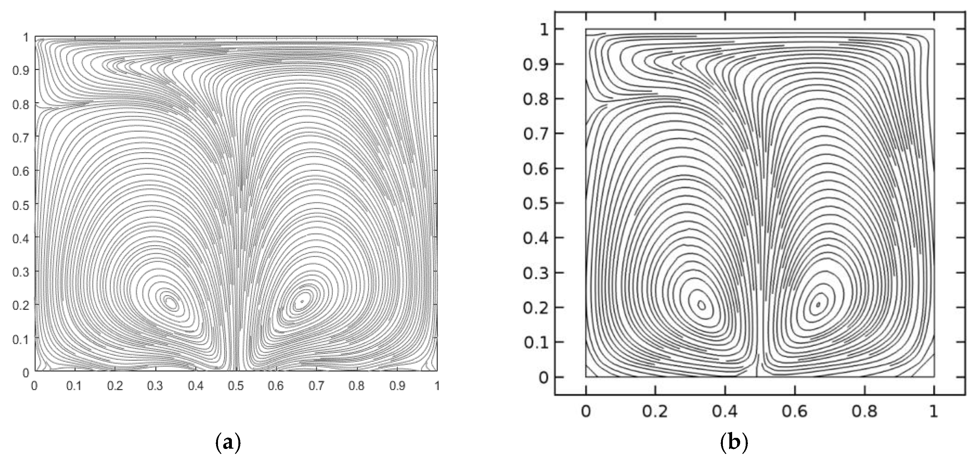
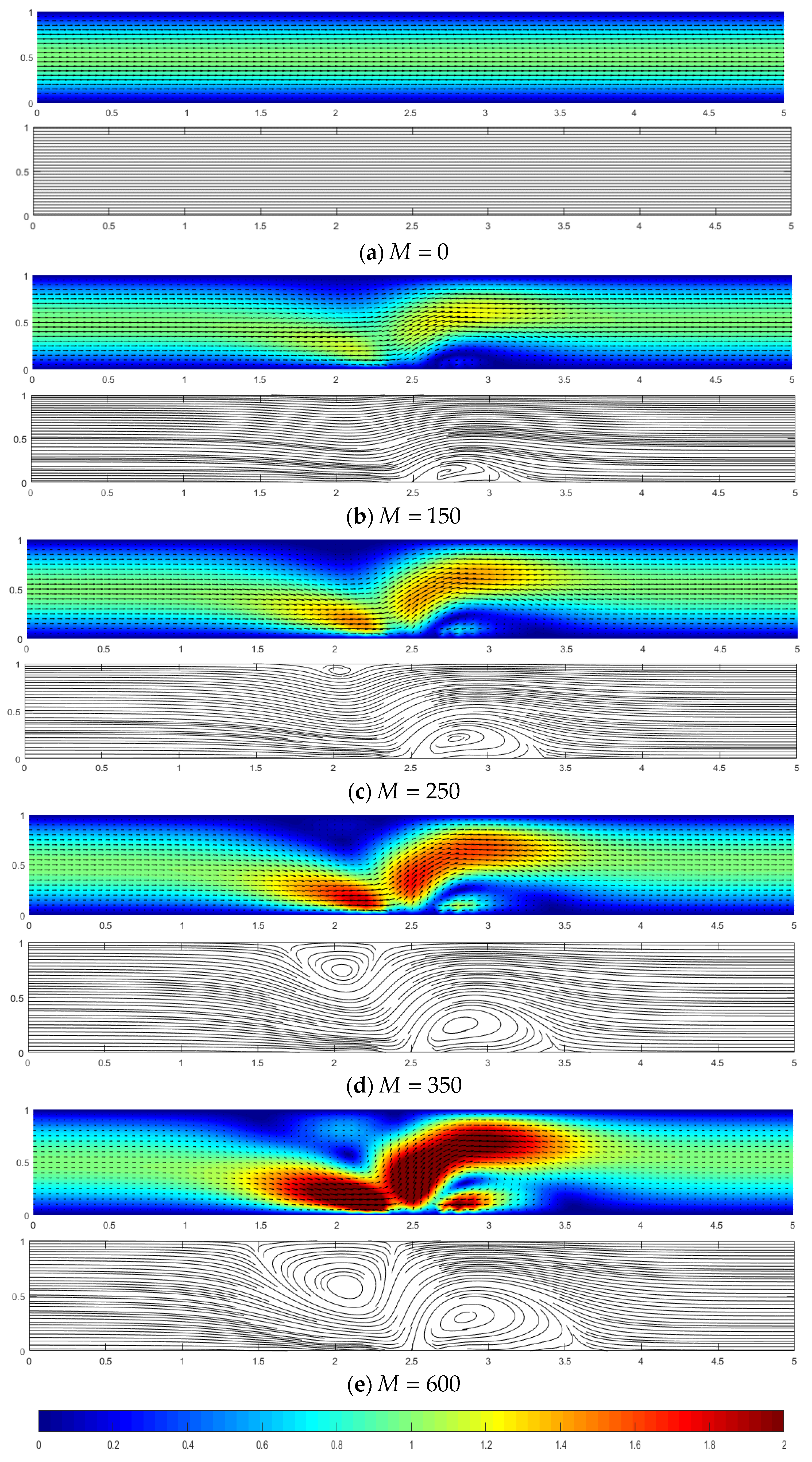
The velocity contour and streamline pattern for the Stokes flow subjected to various magnetic field numbers are presented in Figure 8. When the magnetic field was not imposed $(M=0)$, fluid flow moved in parallel. When the magnetic source was applied at the lower wall, a small vortex formed at the area where the point-source magnetic field was located. Starting from $M=150$, the applied point-source magnetic field disturbed the flow. When the magnetic number increased to 250, a new vortex formed at the upper wall of the channel, while the vortex at the lower wall grew. Starting with $M=250$, the height and length of the vortex at both the lower and upper walls of the channel increased with the increment of magnetic number.

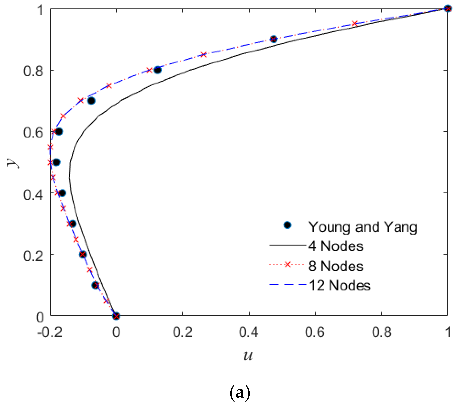
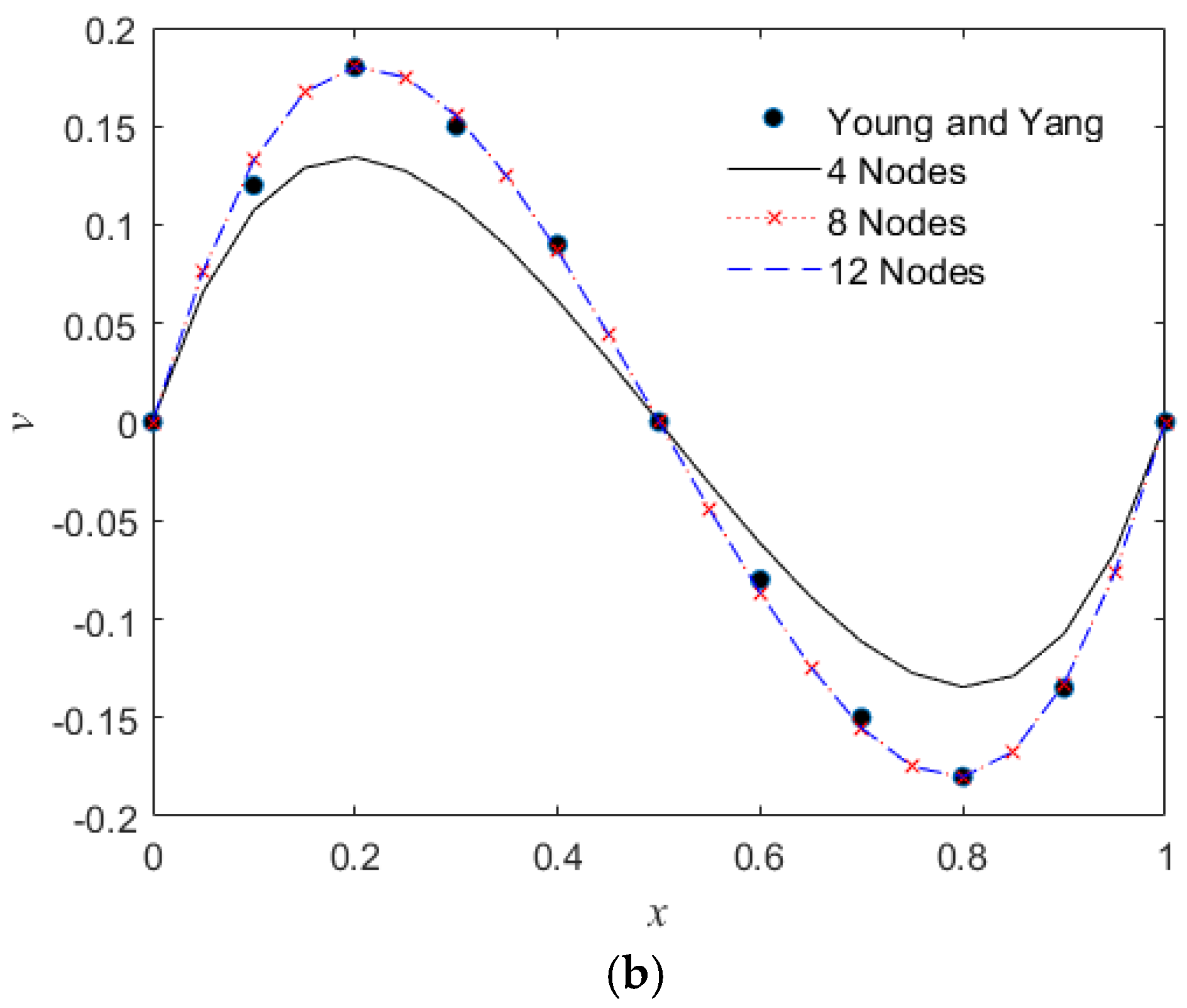
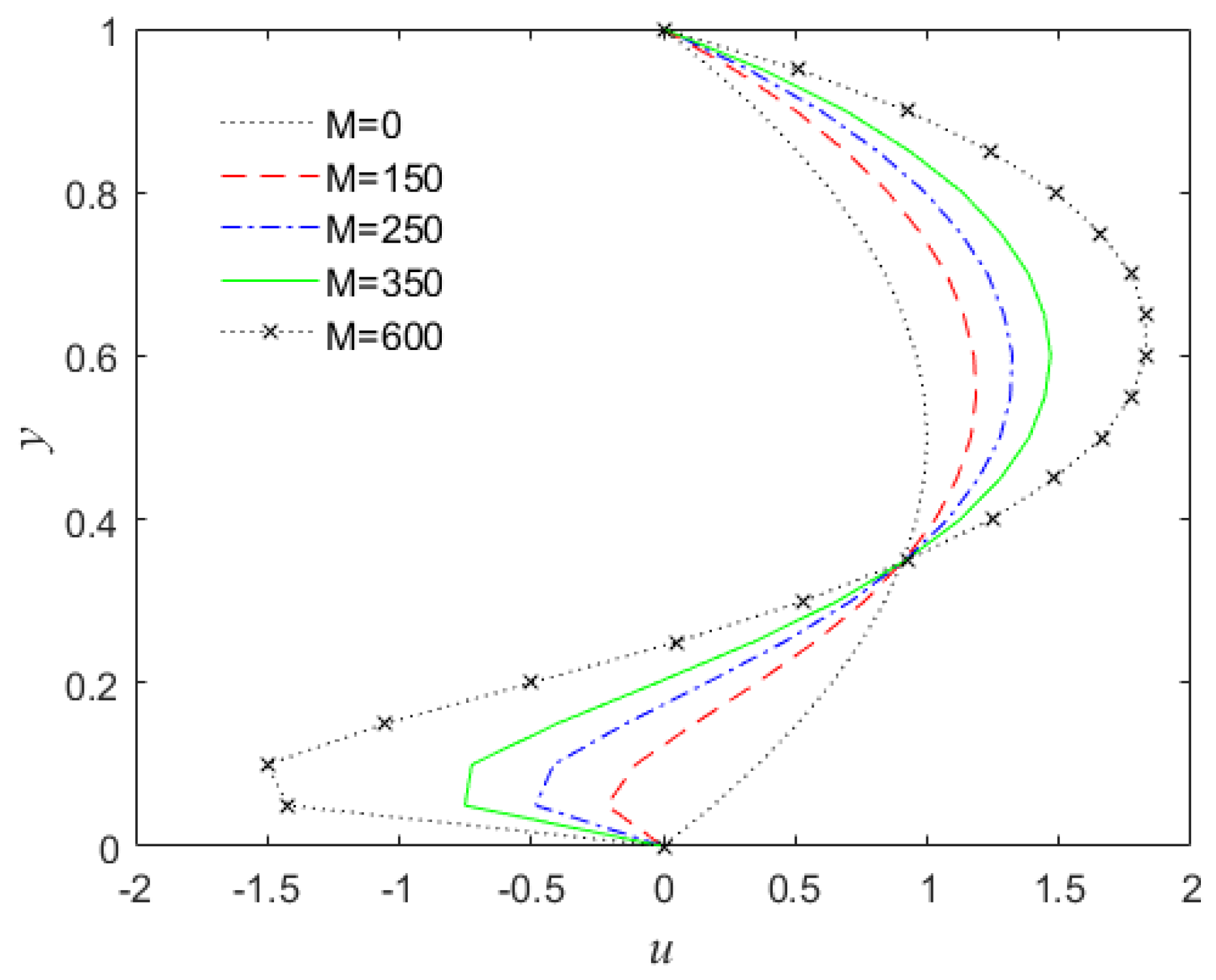
Figure 9 presents the u-velocity profiles along y for different magnetic numbers. The velocity profile changed form when a magnetic field was applied, as can be seen here. Due to the magnetic field action, a vortex formed on the bottom wall. Additionally, when the number of magnetic fields grew, maximal velocity also increased.

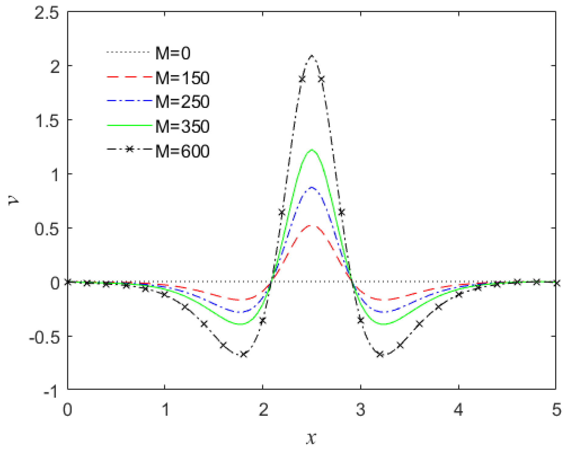
The comparison of the v-velocity profile along the channel at y = 0.5 for different magnetic numbers is shown in Figure 10, where the axial velocity took the same shape for all cases except for flow without a magnetic field. Flow with a magnetic field showed that velocity flow retained a constant value at the beginning of the flow; then, velocity dropped before the point of the magnetic source was applied. As the flow approached the source of the magnetic field, velocity increased to the maximum. Maximal velocity for all cases of flow with a magnetic field was observed at x = 2.5 where the point-source magnetic field was located. Velocity dropped again after passing through the magnetic field source and then remained constant until the exit. Axial velocity for flow under the effect of the point-source magnetic field demonstrated that the minimal velocity values before and after the magnetic field source were the same.

6. Conclusions

This work effectively modelled the Stokes equation with a point-source magnetic field using the least-squares finite element method. Governing equations were recast into an analogous first-order system by introducing an extra independent variable, vorticity. As a result, researchers concentrate on first-order systems that employ the velocity–vorticity formulation. The Stokes problem can be easily solved using the least-squares approach. The development of MATLAB source code is indirectly simplified. The LSFEM, on the other hand, has a problem with locking nodal expansions at low orders. The present study proposed a solution for this problem where the domain of the problem is discretized using higher-order element nodes without applying the reduced integration technique. Thus, the 12-node serendipity element must be used to obtain acceptable numerical results.

The numerical simulation of Stokes flow in a straight rectangular channel under a point-source magnetic field was carried out, and the findings of the velocity contour and streamlines pattern were observed and analysed. Incorporating a magnetic field alters the flow behaviour. After applying a magnetic field, a single vortex could be seen on the lower wall. In response to an increase in magnetic number, a new vortex formed at the channel’s upper wall. As the number of magnetic fields rose, vortices dramatically grew. Results signify the use of LSFEM as an alternative for modelling Stokes flow problems. This work is considered to be the first implementation of the least-squares finite element method on solving Stokes flow in the straight rectangular channel under a point-source magnetic effect. No study has investigated the magnetic effect for Stokes flow in a straight channel. The closest study is by [27], where the magnetic effect was investigated on the basis of the Navier–Stokes equation using a finite difference method. The current study focused on solving the Stokes flow with a magnetic effect using LSFEM. Observed results by this study and by [27] in terms of magnetic strength had a similar effect on the lower wall of the channel.

The LSFEM was successfully employed for the solution of Stokes equations; hence, the LSFEM is proposed for solving the Navier–Stokes equation with and without a magnetic effect for future work. This would allow for the inclusion of convection acceleration and nonlinearity of the solution.

References

1. Eldho, T.; Young, D.L. Solution of Stokes flow problem using dual reciprocity boundary element method. J. Chin. Inst. Eng. 2001, 24, 141–150. [Google Scholar] [CrossRef]
2. Trombley, C.I.; Ekiel-Jeżewska, M.L. Basic concepts of stokes flows. In Flowing Matter; Springer: Cham, Switzerland, 2019; pp. 35–50. [Google Scholar]
3. Young, D.; Tsai, C.; Eldho, T.; Cheng, A.-D. Solution of Stokes flow using an iterative DRBEM based on compactly-supported, positive-definite radial basis function. Comput. Math. Appl. 2002, 43, 607–619. [Google Scholar] [CrossRef] [Green Version]
4. Galaktionov, O.; Meleshko, V.; Peters, G.; Meijer, H. Stokes flow in a rectangular cavity with a cylinder. Fluid Dyn. Res. 1999, 24, 81. [Google Scholar] [CrossRef]
5. Young, D.; Jane, S.; Lin, C.; Chiu, C.; Chen, K. Solutions of 2D and 3D Stokes laws using multiquadrics method. Eng. Anal. Bound. Elem. 2004, 28, 1233–1243. [Google Scholar] [CrossRef]
6. Young, D.; Jane, S.; Fan, C.-M.; Murugesan, K.; Tsai, C. The method of fundamental solutions for 2D and 3D Stokes problems. J. Comput. Phys. 2006, 211, 1–8. [Google Scholar] [CrossRef]
7. Ali, F.; Sheikh, N.A.; Khan, I.; Saqib, M. Magnetic field effect on blood flow of Casson fluid in axisymmetric cylindrical tube: A fractional model. J. Magn. Magn. Mater. 2017, 423, 327–336. [Google Scholar] [CrossRef]
8. Shaw, S.; Murthy, P. Magnetic drug targeting in the permeable blood vessel—The effect of blood rheology. J. Nanotechnol. Eng. Med. 2010, 1, 021001. [Google Scholar] [CrossRef]
9. Banerjee, M.K.; Datta, A.; Ganguly, R. Magnetic drug targeting in partly occluded blood vessels using magnetic microspheres. J. Nanotechnol. Eng. Med. 2010, 1, 041005. [Google Scholar] [CrossRef]
10. Ganguly, R.; Gaind, A.P.; Sen, S.; Puri, I.K. Analyzing ferrofluid transport for magnetic drug targeting. J. Magn. Magn. Mater. 2005, 289, 331–334. [Google Scholar] [CrossRef]
11. Rosensweig, R.E. Ferrohydrodynamics; Courier Corporation: North Chelmsford, MA, USA, 2013. [Google Scholar]
12. Sellier, A.; Aydin, S.; Tezer-Sezgin, M. Free-space fundamental solution of a 2D steady slow viscous MHD flow. Comput. Model. Eng. Sci. 2014, 102, 393–406. [Google Scholar]
13. Gürbüz, M.; Tezer-Sezgin, M. MHD Stokes flow in lid-driven cavity and backward-facing step channel. Eur. J. Comput. Mech. 2015, 24, 279–301. [Google Scholar] [CrossRef]
14. Gürbüz, M.; Tezer-Sezgin, M. MHD Stokes flow in a smoothly constricted rectangular enclosure. In Proceedings of the Conference on Advances in Boundary Element & Meshless Techniques XVII (BETEQ), Ankara, Turkey, 11–13 July 2016; pp. 73–78. [Google Scholar]
15. Gürbüz, M.; Tezer Sezgin, M. RBF solutıon of MHD stokes flow and MHD flow in a constricted enclosure. J. Appl. Eng. Math. 2021, 11, 203–215. [Google Scholar]
16. Senel, P.; Tezer-Sezgin, M. DRBEM solutions of Stokes and Navier–Stokes equations in cavities under point source magnetic field. Eng. Anal. Bound. Elem. 2016, 64, 158–175. [Google Scholar] [CrossRef]
17. Türk, Ö. An MHD Stokes eigenvalue problem and its approximation by a spectral collocation method. Comput. Math. Appl. 2020, 80, 2045–2056. [Google Scholar] [CrossRef]
18. Bramble, J.; Schatz, A. On the numerical solution of elliptic boundary value problems by least squares approximation of the data. In Numerical Solution of Partial Differential Equations—II; Elsevier: Amsterdam, The Netherlands, 1971; pp. 107–131. [Google Scholar]
19. Bo-Nan, J.; Chang, C. Least-squares finite elements for the Stokes problem. Comput. Methods Appl. Mech. Eng. 1990, 78, 297–311. [Google Scholar] [CrossRef]
20. Bochev, P.B.; Gunzburger, M.D. A least-squares finite element method for the Navier-Stokes equations. Appl. Math. Lett. 1993, 6, 27–30. [Google Scholar] [CrossRef] [Green Version]
21. Jiang, B.-N.; Povinelli, L.A. Least-squares finite element method for fluid dynamics. Comput. Methods Appl. Mech. Eng. 1990, 81, 13–37. [Google Scholar] [CrossRef] [Green Version]
22. Carey, G.F.; Jiang, B.N. Element-by-element linear and nonlinear solution schemes. Commun. Appl. Numer. Methods 1986, 2, 145–153. [Google Scholar] [CrossRef]
23. Fortin, M.; Brezzi, F. Mixed and Hybrid Finite Element Methods; Springer: New York, NY, USA, 1991. [Google Scholar]
24. Shui, Q.-X.; Wang, D.-G.; He, Z.-L.; Huang, J. Least square finite element method for viscous splitting of unsteady incompressible Navier–Stokes equations. China Ocean Eng. 2018, 32, 490–500. [Google Scholar] [CrossRef]
25. Reddy, J.N.; Gartling, D.K. The Finite Element Method in Heat Transfer and Fluid Dynamics; CRC Press: Boca Raton, FL, USA, 2010. [Google Scholar]
26. Young, D.; Liu, Y.; Eldho, T. Three-dimensional Stokes flow solution using combined boundary element and finite element methods. J. Mech. 1999, 15, 169–176. [Google Scholar] [CrossRef]
27. Loukopoulos, V.; Tzirtzilakis, E. Biomagnetic channel flow in spatially varying magnetic field. Int. J. Eng. Sci. 2004, 42, 571–590. [Google Scholar] [CrossRef]
Figure 1. Problem domain and boundary conditions.
Symmetry 14 00514 g001
Figure 2. (a) Mesh; (b) boundary conditions for the lid driven cavity flow.
Symmetry 14 00514 g002
Figure 3. Comparison for (a) u-central velocity along y and (b) v-central velocity along x between [26] and the present study.
Symmetry 14 00514 g003aSymmetry 14 00514 g003b
Figure 4. Stokes flow with a point source magnetic field. (a) Problem domain and boundary condition; (b) magnetic field intensity.
Symmetry 14 00514 g004
Figure 5. Comparison of (a) u-central velocity and (b) v-central velocity for M = 10,000 between COMSOL Multiphysics and present study.
Symmetry 14 00514 g005
Figure 6. Streamline pattern obtained from (a) present study and (b) COMSOL for M = 10,000 .
Symmetry 14 00514 g006
Figure 7. Geometry of rectangular channel. (a) Problem domain and boundary condition; (b) mesh.
Symmetry 14 00514 g007
Figure 8. Velocity contour and streamline pattern for Stokes flow subjected to magnetic field in straight rectangular channel at various magnetic numbers M .
Symmetry 14 00514 g008
Figure 9. u-velocity profiles along y at x = 2.7 subjected to various magnetic number.
Symmetry 14 00514 g009
Figure 10. v-velocity profiles along x at y = 0.5 of channel subjected to various magnetic numbers.
Symmetry 14 00514 g010
Publisher’s Note: MDPI stays neutral with regard to jurisdictional claims in published maps and institutional affiliations.