
Exact Treatment of the Ground States of Three Two-Dimensional Contact Interactions in a Uniform Magnetic Field

Abstract
:1. Introduction
2. Green Function
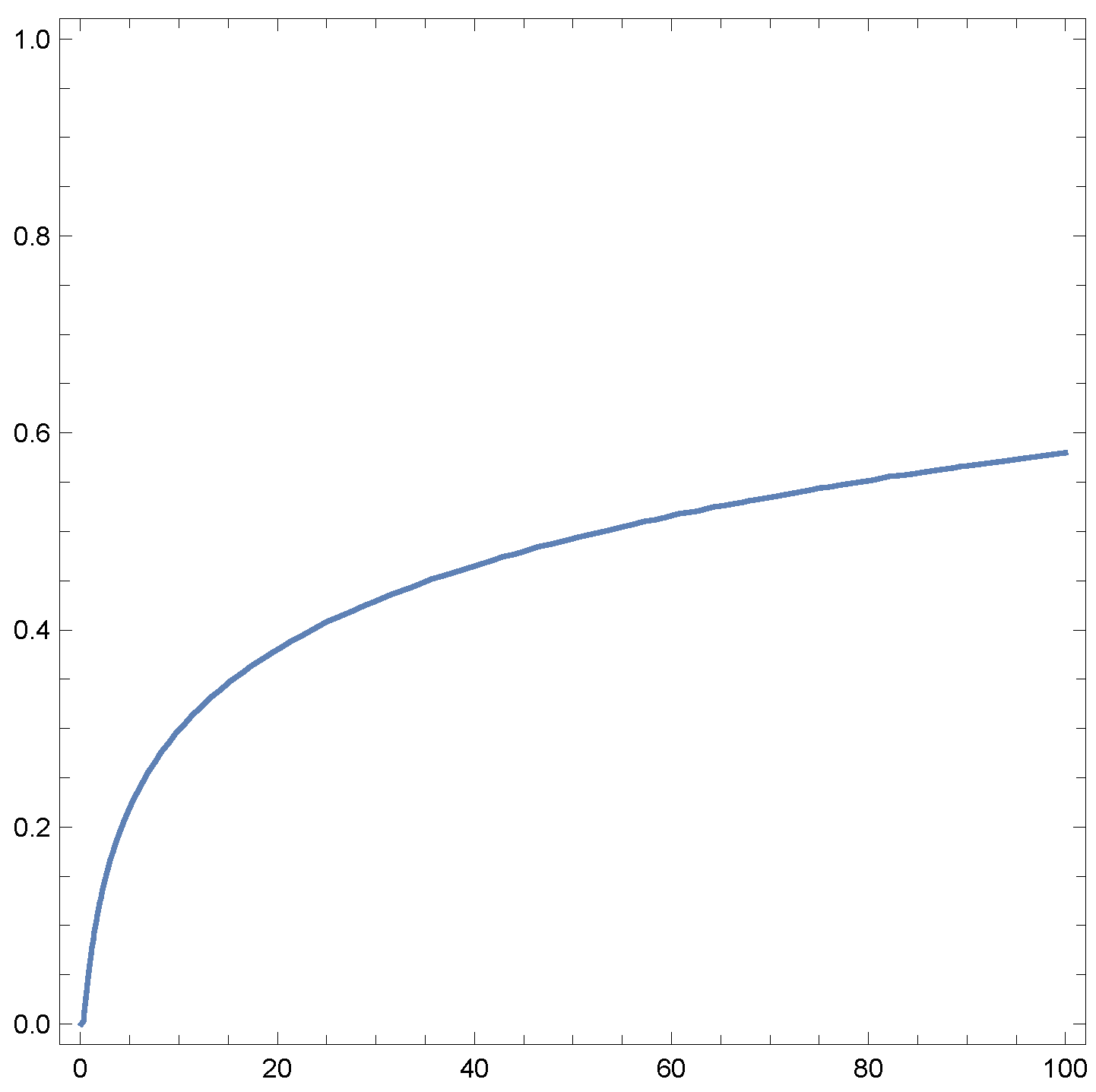
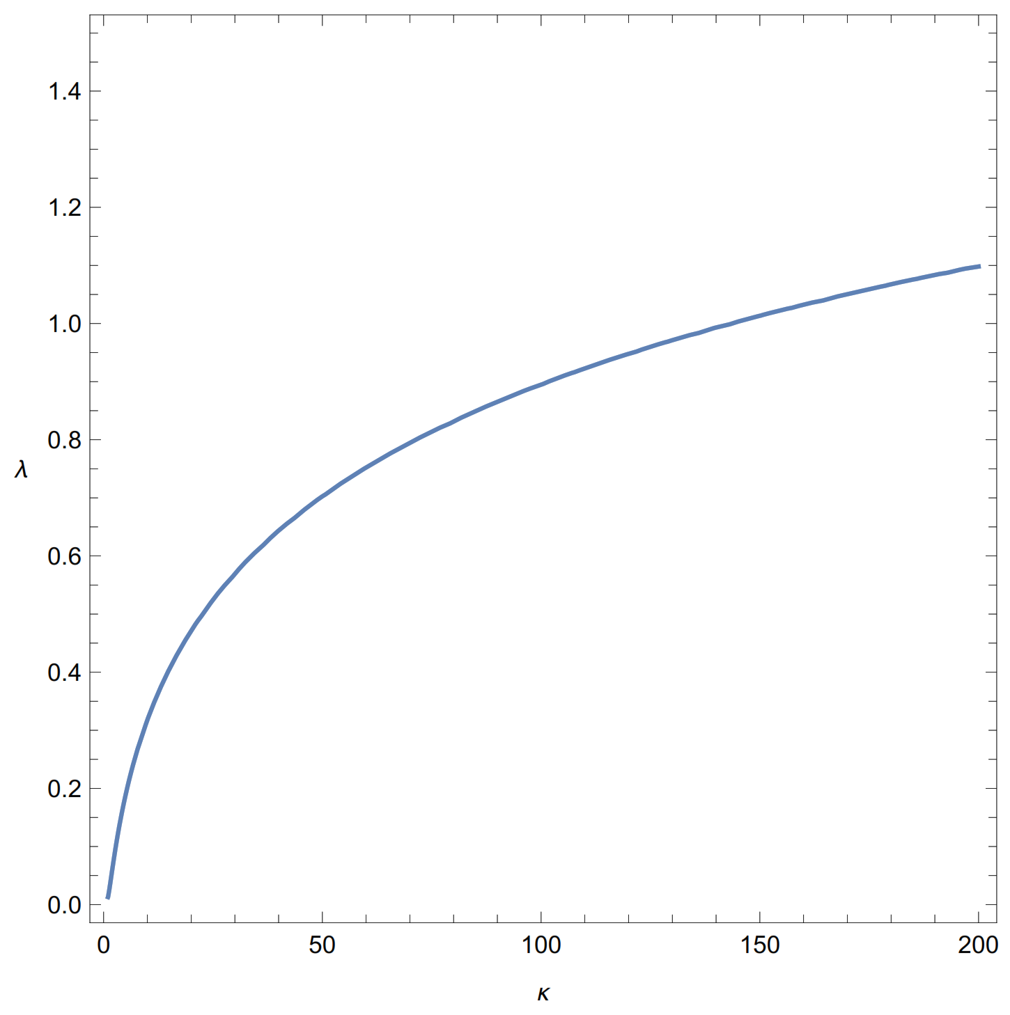
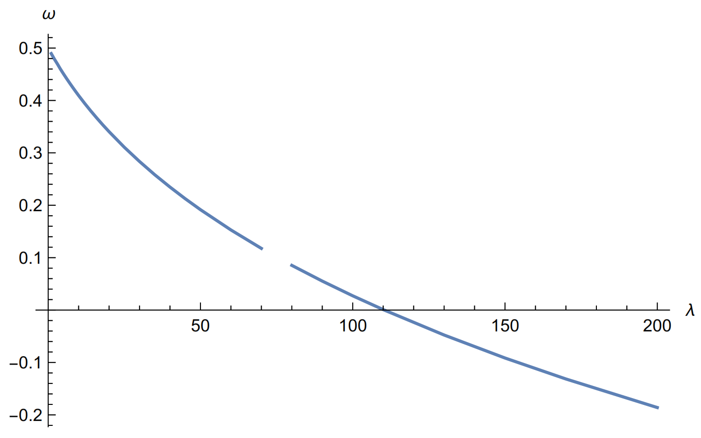
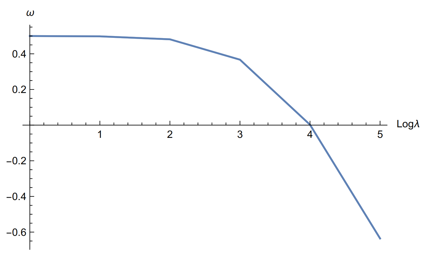
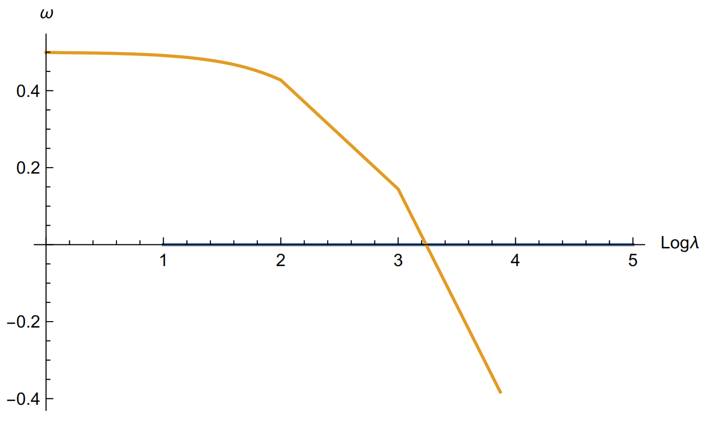
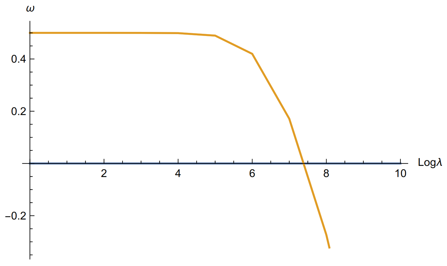
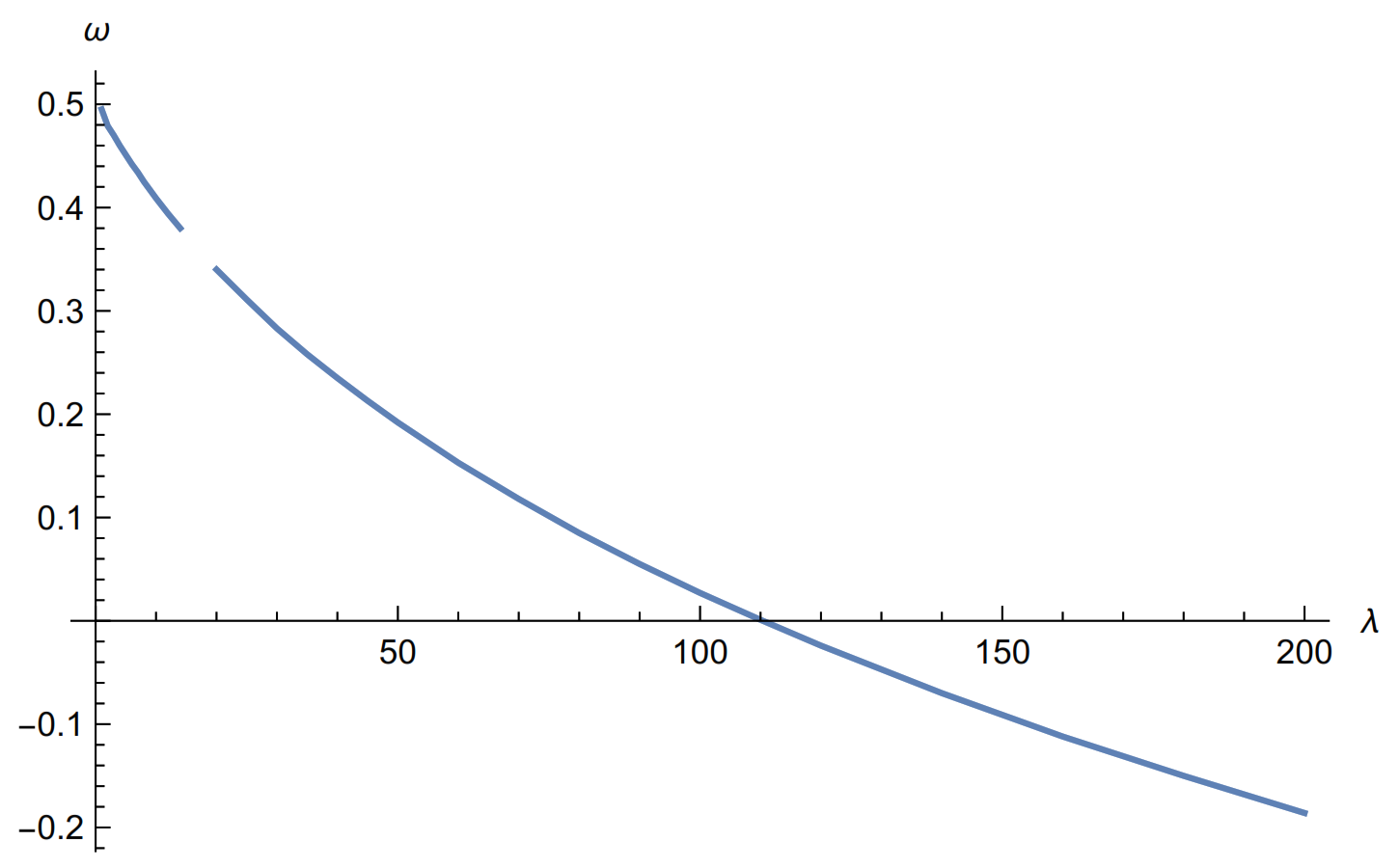
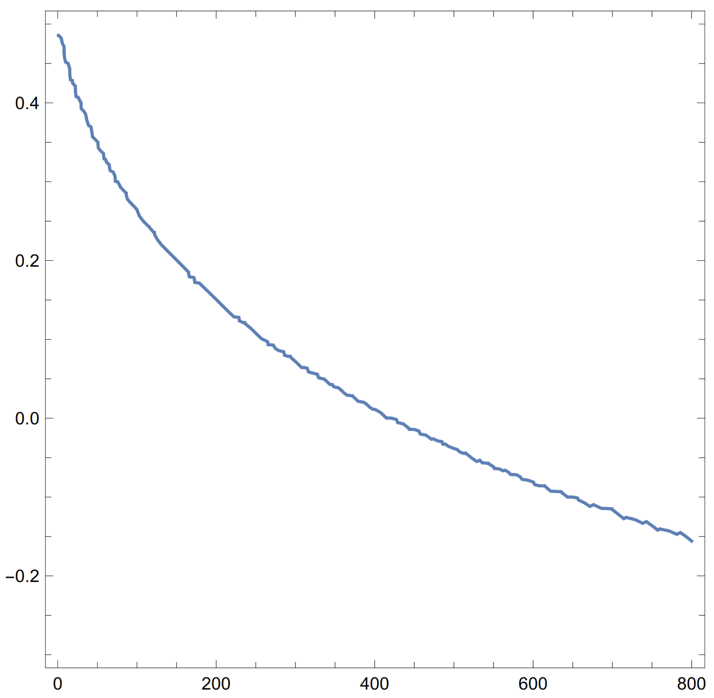
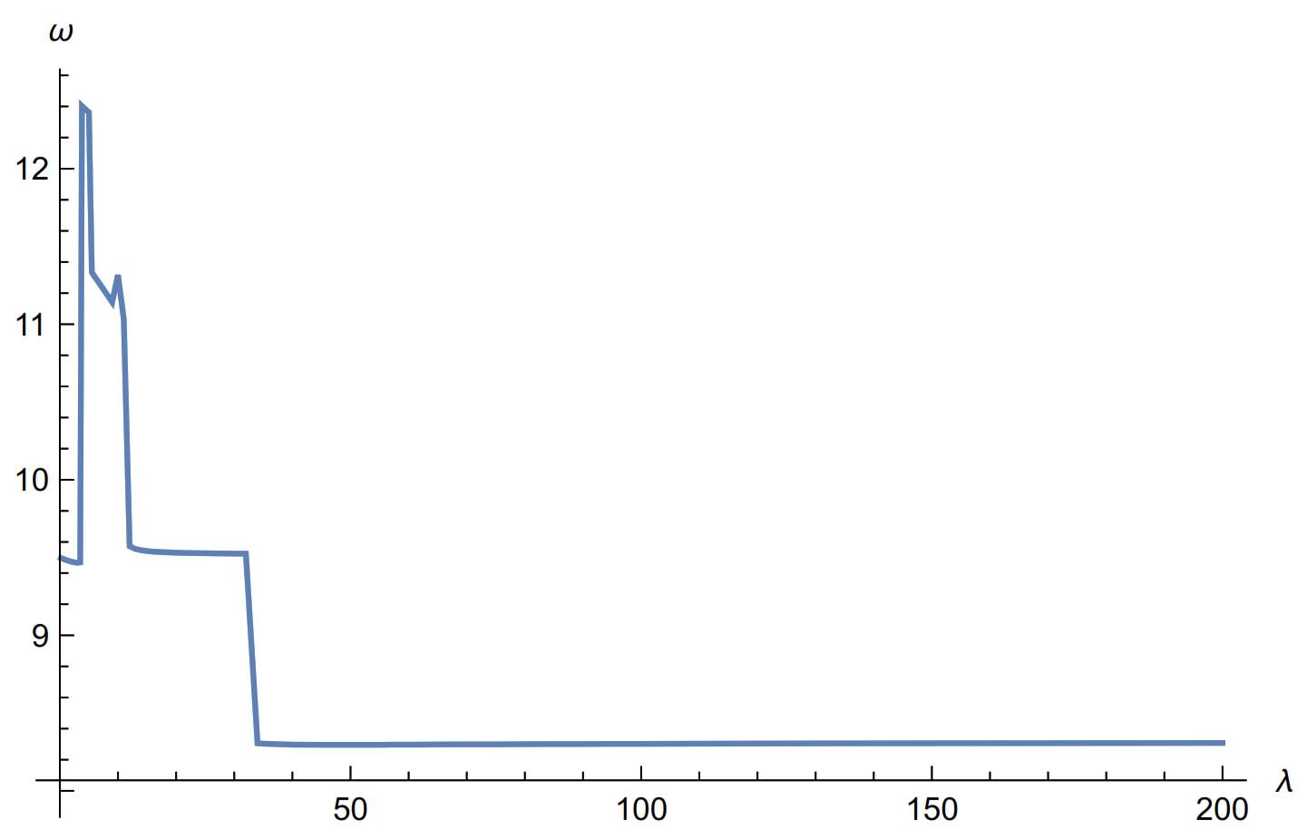
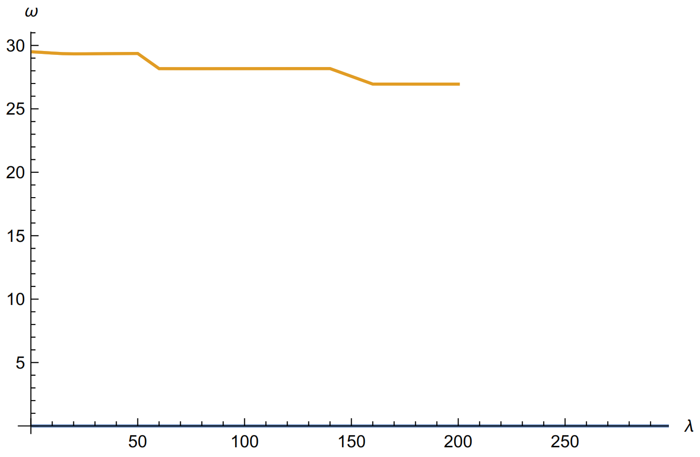
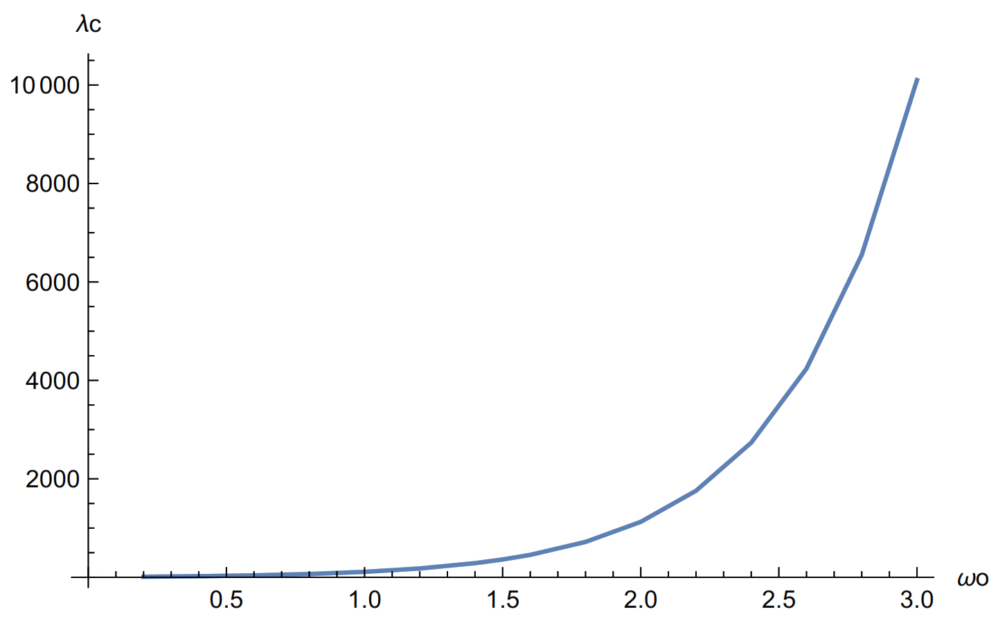
3. Calculation
4. Conclusions
Funding
Institutional Review Board Statement
Informed Consent Statement
Acknowledgments
Conflicts of Interest
Appendix A
References
- Horing, N.J.M. Quantum Statistical Field Theory; Oxford University Press: Oxford, UK, 2017; Section 12.4. [Google Scholar]
- Horing, N.J.M.; Mancini, J.D.; Horton, S.L. Landau Quantized Dynamics and Energy Spectra of Asymmetric Double-Quantum- MDF Systems: (a) Non-Relativistic Electrons; (b) Dirac T-3 Diced Lattice Carriers", Chapter 13 in "Progress in Nanoscale and Low Dimensional Materials and Devices; Springer Nature Series “Topics in Applied Physics”; Springer: Berlin/Heidelberg, Germany, in press.
- Harrison, P. Quantum Wells, Wires and Dots, 3rd ed.; John Wiley and Sons, Ltd.: Hoboken, NJ, USA, 2009. [Google Scholar]
- Jacak, L.; Hawrylak, P.; Wois, A. Quantum MDFs; Springer: Berlin, Germany, 1998. [Google Scholar]
- Albeverio, S. Solvable Models in Quantum Mechanics; Springer: Berlin, Germany, 1988. [Google Scholar]
- Titchmarsh, E.C. Eigenvalue Expansions; Clarendon University Press: Oxford, UK, 1946; Section 4.2. [Google Scholar]
- Sondheimer, E.H.; Wilson, A.H. The Diamagnetism of Free Electrons. Proc. R. Soc. Lond. Ser. A 1951, 210, 173–190. [Google Scholar]
- Glasser, M.L. Summation over Feynman Histories: Charged Particle in a Uniform Magnetic Field. Phys. Rev. 1964, 133, B831. [Google Scholar] [CrossRef]
- Ueta, T. Green Function of a Charged Particle in Magnetic Fields. J. Phys. Soc. Jpn. 1992, 61, 4314–4324. [Google Scholar] [CrossRef]
- Kubo, R.; Mitake, S.J.; Hashitsume, N. Solid State Physics; Seitz, F., Turnbull, D., Eds.; Academic Press: New York, NY, USA, 1965; Volume 17, p. 362. [Google Scholar]
- Horing, N.J.M. Quantum Statistical Field Theory; Oxford Science Publications: Oxford, UK, 2017; Chapter 5. [Google Scholar]
- Cresti, A.; Grosso, G.; Parravincini, G.P. Analytic and Numeric Green Functions for a Two-Dimensional Electron Gas in an Orthogonal Magnetic Field. Ann. Phys. 2006, 321, 1075–1091. [Google Scholar] [CrossRef]
- Handbook of Mathematical Functions; NBS Appl. Math. Series 55; Abramowitz, M.; Stegun, I. (Eds.) Forgotten Books: Washington, DC, USA, 1964; p. 504. [Google Scholar]
- Glasser, M.L. A Note on the Exact Green Function for a Quantum System Decorated by Impurities. Front. Phys. 2019, 7, 7. [Google Scholar] [CrossRef] [Green Version]


Publisher’s Note: MDPI stays neutral with regard to jurisdictional claims in published maps and institutional affiliations. |
© 2022 by the author. Licensee MDPI, Basel, Switzerland. This article is an open access article distributed under the terms and conditions of the Creative Commons Attribution (CC BY) license (https://creativecommons.org/licenses/by/4.0/).
Share and Cite
Glasser, M.L. Exact Treatment of the Ground States of Three Two-Dimensional Contact Interactions in a Uniform Magnetic Field. Symmetry 2022, 14, 489. https://doi.org/10.3390/sym14030489
Glasser ML. Exact Treatment of the Ground States of Three Two-Dimensional Contact Interactions in a Uniform Magnetic Field. Symmetry. 2022; 14(3):489. https://doi.org/10.3390/sym14030489
Chicago/Turabian StyleGlasser, Mervyn Lawrence. 2022. "Exact Treatment of the Ground States of Three Two-Dimensional Contact Interactions in a Uniform Magnetic Field" Symmetry 14, no. 3: 489. https://doi.org/10.3390/sym14030489