Article

Assembly Configuration Representation and Kinematic Modeling for Modular Reconfigurable Robots Based on Graph Theory

1
Ningbo Institute of Materials Technology and Engineering, Chinese Academy of Sciences, Ningbo 315201, China
2
Zhejiang Key Laboratory of Robotics and Intelligent Manufacturing Equipment Technology, Ningbo 315201, China
3
University of Chinese Academy of Sciences, Beijing 100049, China
*
Author to whom correspondence should be addressed.
Symmetry 2022, 14(3), 433; https://doi.org/10.3390/sym14030433
Submission received: 6 January 2022 / Revised: 3 February 2022 / Accepted: 19 February 2022 / Published: 22 February 2022
(This article belongs to the Special Issue Graph Algorithms and Graph Theory)

Abstract

:
A Modular Reconfigurable Robot (MRR) composed of standard joint and link modules has the advantages of rapid changeover of assembly configurations for a diversity of application requirements. To tackle the kinematics analysis issues for an MRR, it is essential to develop a generic method to mathematically represent all possible assembly configurations and automatically generate their kinematic models. In this paper, two types of robot modules, i.e., revolute joint modules and rigid link modules, are considered as the basic building blocks of an MRR. The topological structure of an MRR is represented by a graph, termed an Assembly Graph (AG), in which all robot modules, regardless of their types, are treated as vertices, while the connecting interfaces between any two robot modules are treated as edges. Based on graph theory, a modified adjacency matrix, termed an Assembly Adjacency Matrix (AAM), is proposed to represent the assembly configuration of an MRR, in which the three-dimensional assembly information is specified with connecting port vectors for the adjacent modules. A path matrix derived from the AAM of an MRR is employed to describe the connecting sequence of its constituting modules. The local frame representation of the Product-of-Exponentials (POE) formula is employed, which is configuration-independent. Therefore, for an MRR configuration represented with an AAM, its kinematic model will be automatically generated according to its path matrix. The proposed assembly configuration representation and kinematic modeling method are validated through a dual-branch MRR configuration.

1. Introduction

Conventional monolithically designed industrial robots have been widely employed in high-volume production owing to their high productivity in performing repetitive tasks [1]. However, due to their fixed configurations, the conventional industrial robots are unable to meet the ever-changing task requirements in today’s high-mix low-volume manufacturing scenarios. To tackle such difficulties, a Modular Reconfigurable Robot (MRR) composed of standard joint and link modules is a promising solution, as it has the advantages of rapid changeover of assembly configurations for a diversity of application requirements.
In recent years, MRRs have received significant attention from both research communities and industries, and a variety of MRRs have been developed. Kelmar et al. [2,3] proposed an MRR termed the Reconfigurable Modular Manipulator System (RMMS), which consists of revolute joint modules and link modules with different sizes. Singh et al. [4,5] developed a Spring-Assisted Modular and Reconfigurable Robot (SA-MRR), in which each joint module has two working modes, i.e., the normal working mode and the spring-assisted working mode, through a brake-spring assembly for safe manipulation. Liu et al. [6,7] designed a Self-assembling MOdular Robot for Extreme Shapeshifting (SMORES), which consists of several versatile 4-DOF joint modules for self-assembly. Zhao et al. [8] designed an astronaut robotic limb system (AstroLimbs) for astronaut activity assistance, which is composed of identical revolute joint modules with three initial configurations based on a triangular prism design. The German company SCHUNK [9] commercialized a modular robot system, termed Powerball LWA, which consists of two types of joint modules, i.e., 1-DOF revolute joint modules and 2-DOF revolute joint modules, for industrial applications. As an MRR is composed of standard joint and link modules, its performance is module-dependent. Significant research efforts have been devoted to the internal mechatronic design and the connecting interface design of the joint and link modules. Dogra et al. [10,11] designed a revolute joint module with a dip axis for unconventional robot manipulators and optimized the module design by considering its dynamics. Yun et al. [12] designed both 1-DOF and 2-DOF joint modules with integrated mechatronic designs and link modules with genderless connectors. Romiti et al. [13] developed a reconfigurable collaborative robot that consists of base modules, straight and elbow joint modules, and tool-exchanger modules. The modules can be quickly connected together through C-couplings and standard electromechanical interfaces.
As an MRR can be assembled into many possible configurations, it is critical to develop a mathematical method to represent the 3D assembly configurations of an MRR so as to facilitate the modeling, analysis, and control issues. Chen and Yang [14] proposed a kinematic graph-based Assembly Incidence Matrix (AIM) to describe the assembly configuration of an MRR, in which the link modules are treated as vertices and the joint modules are treated as edges. Although AIM representation can be employed to describe a branched MRR configuration, the conversion scheme to define a kinematic graph is based on a theoretical assumption such that a joint is connected to two links only and a link may accept more than one joint. In practice, a robot joint module is a physical module that may have more than two connecting interfaces, so that it can also be connected to more than two links. As such, the kinematic graph and its associated AIM are not generic enough to describe all possible MRR configurations. Zhao et al. [15] employed an 8-bit binary code to describe the assembly relationship of an MRR configuration, which is computationally effective. Nainer et al. [16] employed the Unified Robot Description Format (URDF) to directly describe the kinematic parameters of an MRR configuration. Although various symbolic and numerical methods have been proposed to mathematically represent MRR configurations, a more generic method needs to be investigated to represent the 3D assembly configuration of an MRR.
Due to the reconfigurability of an MRR, it is essential to automatically generate its kinematic model for the design, trajectory planning, and motion control of an MRR [17,18,19]. Kelmar et al. [2] proposed an approach based on the Denavit–Hartenberg (D-H) [20] formula to automatically generate the kinematic model for an MRR, in which a kinematic transformation algorithm is proposed to convert module parameters into D-H parameters. Chen and Yang [14,21,22,23,24] proposed a method based on the local frame representation of the Product-of-Exponentials (POE) [25,26] formula to automatically formulate the kinematic models for MRR configurations, in which a dyad kinematics expressing the kinematic transformation of a joint-link assembly was developed. Nainer et al. [16] developed the URDF parameterization approach to generate the kinematic model automatically, in which the D-H, modified D-H, and POE formula parameters can be employed. Although previous formulation approaches were able to automatically generate the kinematic models for MRRs, the kinematic model of each constituting active joint module relies on the geometric relationship of its adjacent joint modules or link modules, which is not module-independent.
Inspired by the work represented in [14], a generic assembly configuration representation method and a configuration-independent kinematic modeling method are proposed for an MRR. Two types of robot modules, i.e., revolute joint modules and rigid link modules with cuboid geometries of different sizes, are considered as the basic building blocks of the MRR, which are abstracted from the existing modular robot manipulators. An Assembly Graph (AG) is proposed to represent the topological structure of an MRR configuration, in which both joint modules and link modules are treated as vertices, regardless of their types, while their connecting interfaces are treated as edges. A modified adjacency matrix, termed an Assembly Adjacency Matrix (AAM), is defined to mathematically represent the 3D assembly of an MRR configuration. The local frame representation of the POE formula is directly applied to each of the joint modules, which is configuration-independent. Utilizing the path matrix derived from the AAM of an MRR configuration, the forward kinematic model of an MRR configuration is automatically generated.
The rest of this paper is organized as follows. In Section 2, to describe various configurations of an MRR, two types of abstracted robot modules, i.e., revolute joint modules and rigid link modules with cuboid geometries, are introduced. The definitions of AG, Extend Adjacency Matrix (EAM), and AAM are given in detail in Section 3. In Section 4, the kinematics of joint modules, the fixed kinematic transformation of link modules, and the fixed kinematic transformation between the two adjacent two modules are presented, followed by an automatic kinematic model generation algorithm developed for general branched MRR configurations. In Section 5, simulation results are presented to validate the proposed algorithm. Section 6 presents the conclusions of this paper.

2. Representation of Robot Modules

A Modular Reconfigurable Robot (MRR) is composed of standard joint and link modules. Although there exist various types of robot modules in MRRs, the revolute joint modules and link modules are the most popular robot modules, which are considered in the proposed MRR to realize dexterous manipulations. To generically represent the assembly configurations for the MRR, each of the abstracted robot modules has a cuboid geometry with multiple connecting interfaces.

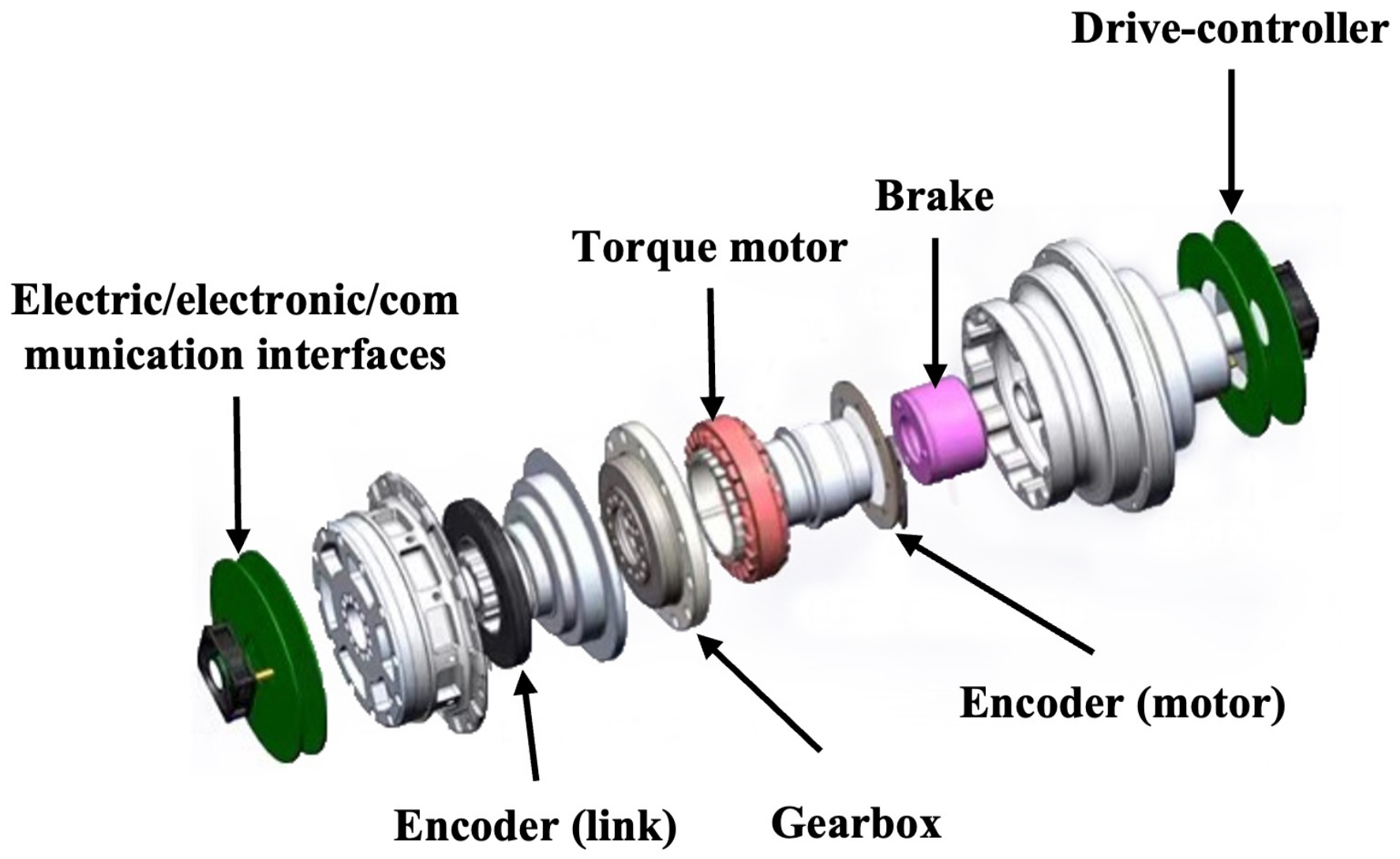
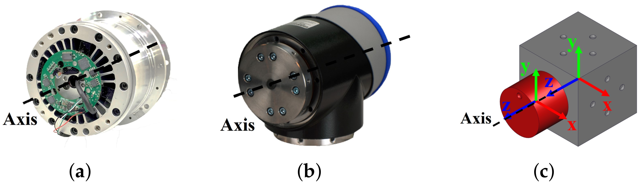
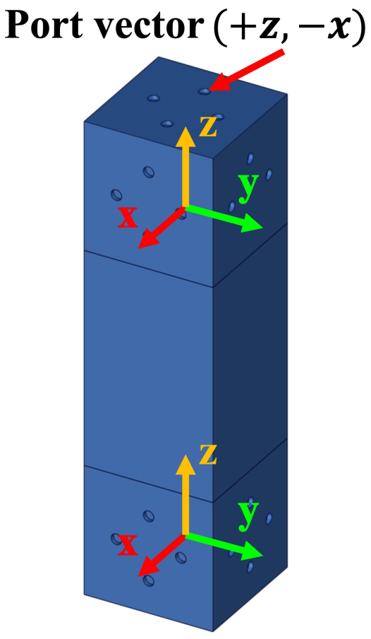
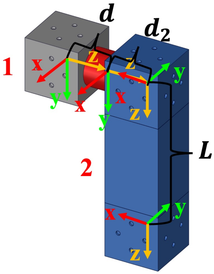
2.1. Revolute Joint Modules
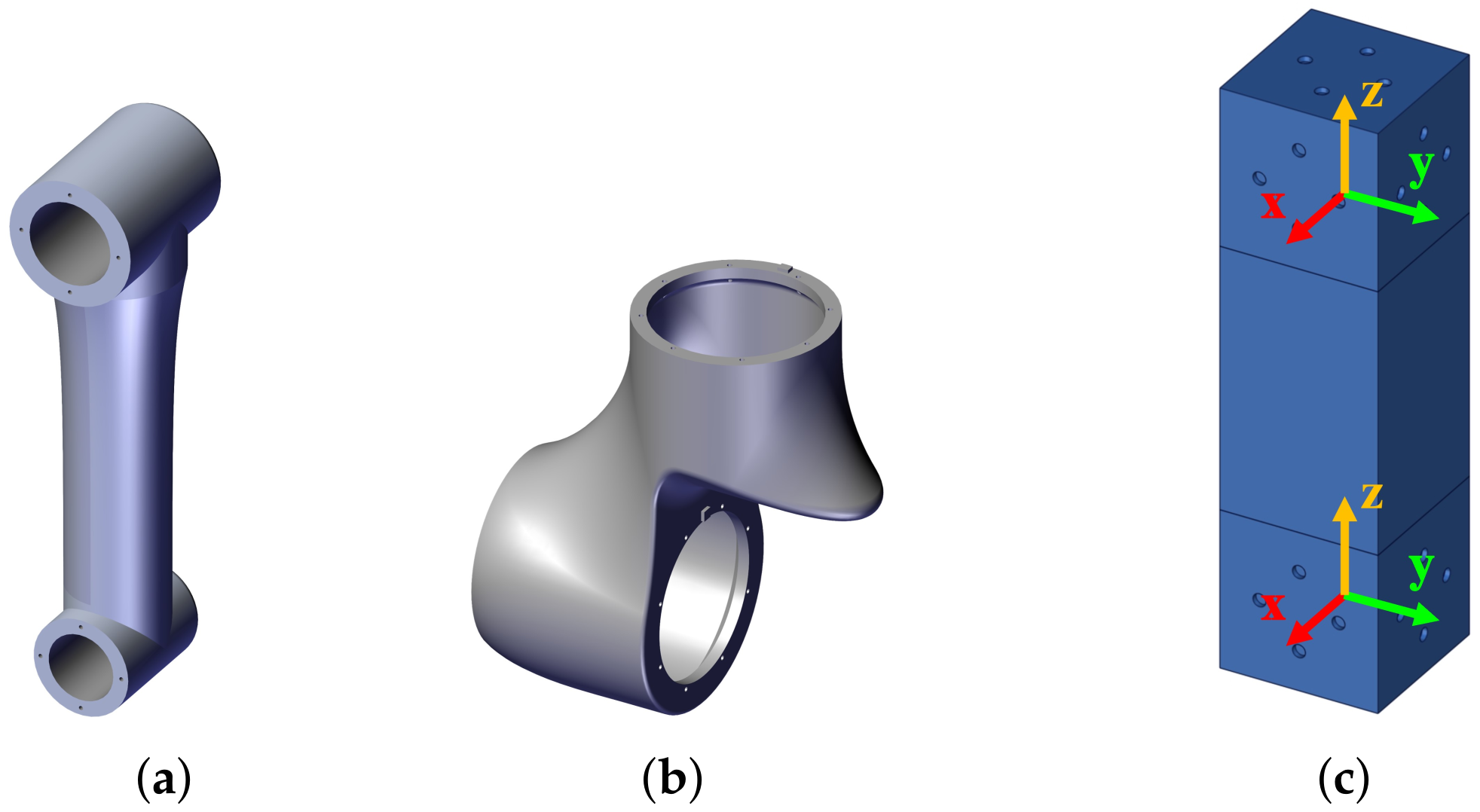
For the existing MRRs, most of their revolute joint modules have adopted a similar integrated mechatronic design. As shown in Figure 1, the internal architecture of a revolute joint module generally consists of a torque motor, a gearbox, a brake, two encoders, a drive controller, and electric/electronic/communication interfaces, which are integrated together to form a self-contained and independent motion control unit. In terms of external designs, two types of revolute joint modules, i.e., the “I” type (as shown in Figure 2a), in which the normals of the two connecting surfaces are coincident with each other, and the “T” type (as shown in Figure 2b), in which the normals of the two connecting surfaces are intersecting and perpendicular with each other, are commonly used. To uniformly represent these two types of revolute joint modules geometrically, a cuboid geometry (as shown in Figure 2c) is proposed, which is a cube with an extrusive solid cylinder. The cube represents the fixed base of the revolute joint module, and it has five connecting surfaces, with four symmetrically distributed location pinholes assigned on each surface. The solid cylinder represents the output shaft of the revolute joint module, which has a connecting flange surface with a location pinhole assigned. Two coordinate frames are assigned on the abstracted revolute joint module to describe the geometric information: one is located on the geometric centers of the cube, and the other is attached to the geometric centers of the cylinder. The two coordinate frames are parallel to each other when the revolute joint module is at its home position. In order to represent the revolute joint modules with different sizes, the cuboid geometry is scalable for small, medium, and large revolute joint modules, denoted by J 1 , J 2 , and J 3 , respectively.

2.2. Link Modules

Two types of link modules with hollow structures are commonly employed in MRRs, i.e., “H” type (as shown in Figure 3a), in which the normals of the two connecting surfaces are parallel to each other, and “L” type (as shown in Figure 3b), in which the normals of the two connecting surfaces are perpendicular to each other. To geometrically represent the link modules uniformly, a cuboid geometry (as shown in Figure 3c) with a cube at each end is employed. For each cube, it has five connecting surfaces, with four symmetrically distributed location pinholes assigned on each surface. Two coordinate frames are assigned on the abstracted link module, with each one on the geometric center of the end cube. The cuboid geometry is also scalable for small, medium, and large link modules, denoted by L 1 , L 2 , and L 3 , respectively.

2.3. Unconventional Modules

In recent years, many unconventional robot modules with a variety of external geometries have been developed, such as 2-DOF joint modules and lightweight link modules [10,11,12,13]. Most of these robot modules can also be represented by the abstracted joint and link modules with cuboid geometries. For example, the 2-DOF joint module in [11] can be represented by an assembly of two abstracted joint modules connected with an abstracted link module, while an unconventional link module [13] can be represented by an assembly of two abstracted link modules.

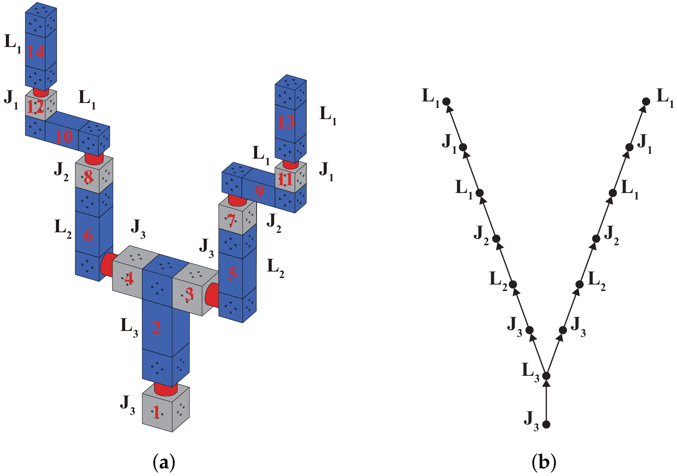
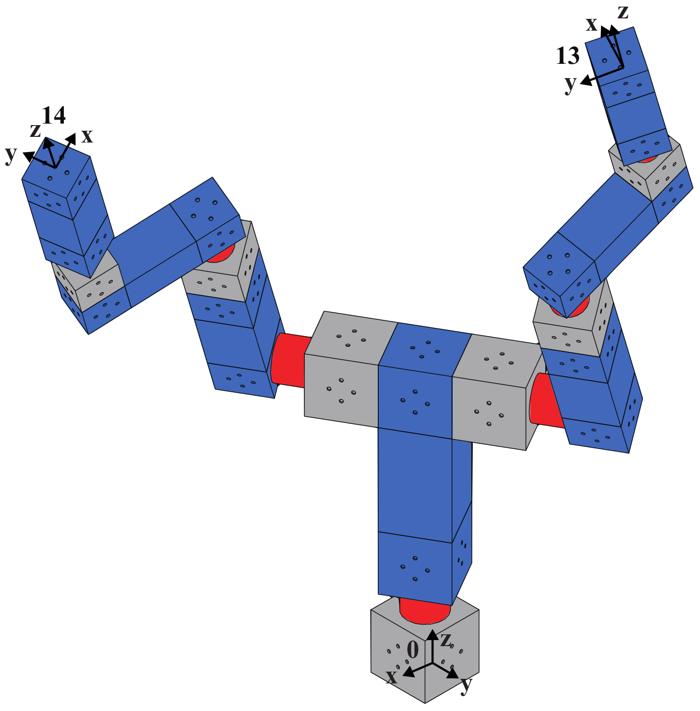
3. MRR Assembly Configuration Representation

To represent the topological structure of an MRR, the Assembly Graph (AG) is proposed, in which all the robot modules are treated as vertices, while the connecting interfaces between any two robot modules are treated as edges. Based on graph theory, the Assembly Adjacency Matrix (AAM) is used to represent the assembly configuration of the MRR in which the three-dimensional assembly information is specified for the adjacent modules.

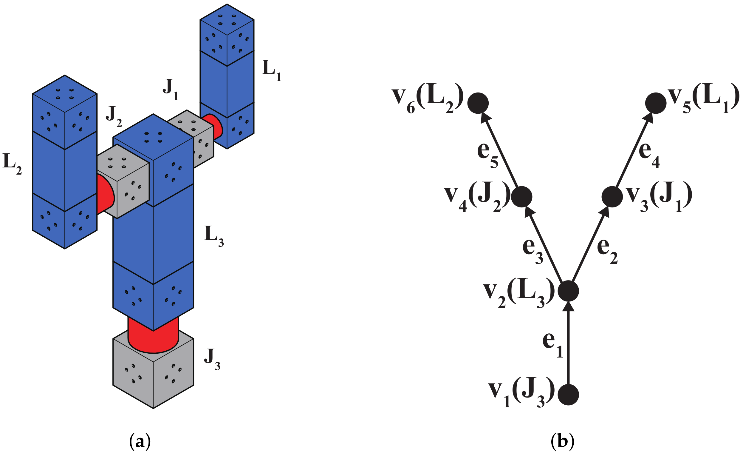
3.1. MRR Assembly Graph

To represent the topological structure of an MRR configuration, the definition of AG is given below.
Definition 1.
The assembly graph is a directed labeled graph G = ( V , E ) , in which the vertex set V { v 1 , v 2 , , v n } is specialized to represent the robot modules such that v i ( i = 1 , 2 , , n ) { J 1 , J 2 , J 3 , L 1 , L 2 , L 3 } , and the edge set E { e 1 , e 2 , , e m } represents the connecting interfaces between two connected robot modules.
For example, a dual-branch MRR assembly configuration that consists of three revolute joint modules with different sizes (i.e., J 1 , J 2 , and J 3 ) and three link modules with different sizes (i.e., L 1 , L 2 , and L 3 ) is shown in Figure 4a, while its AG is shown in Figure 4b.
Based on graph theory, a graph can be represented by its adjacency matrix. As the AG of an MRR assembly configuration is a directed graph, the adjacency matrix ( A ( G ) ) of the AG (as shown in Figure 4) is given by:
A ( G ) = v 1 v 2 v 3 v 4 v 5 v 6 v 1 v 2 v 3 v 4 v 5 v 6 0 1 0 0 0 0 0 0 1 1 0 0 0 0 0 0 1 0 0 0 0 0 0 1 0 0 0 0 0 0 0 0 0 0 0 0
Based on the adjacency matrix of an AG, its accessibility matrix C ( G ) and path matrix P ( G ) can be derived with the following process:
1.
C ( G ) = A ( G ) + A ( G ) 2 + + A ( G ) n 1 , in which n is the number of vertices;
2.
U ( G ) = C ( G ) + I n × n ;
3.
If the entries in row i of C ( G ) are not all equal to 0, delete column i of U ( G ) ;
4.
P ( G ) is given by the transpose of the resulting U ( G ) .
As a computation example, the path matrix of the AG (as shown in Figure 4) is given by:
P ( G ) = v 1 v 2 v 3 v 4 v 5 v 6 p 1 p 2 1 1 1 0 1 0 1 1 0 1 0 1

3.2. Assembly Adjacency Matrix

The adjacency matrix of an AG can only represent the adjacent relationship of vertices (robot modules). To represent the types and sizes of robot modules as well as the input and output ports of the modules, the Extended Adjacency Matrix (EAM) is proposed, which is defined as follows.
Definition 2.
The Extended Adjacency Matrix (EAM) of an AG, denoted by E A ( G ) , is an ( n + 1 ) × n matrix such that:
  • Let a i , j   ( i = 1 , 2 , , n ; j = 1 , 2 , , n ) be the entries of the adjacency matrix, and a ^ i , j be the entries of the extend adjacency matrix;
  • a ^ i , j = a ^ j , i = a i , j   ( i = 1 , 2 , , n ; j = 1 , 2 , , n ) ;
  • a ^ n + 1 , i = v i { J 1 , J 2 , J 3 , L 1 , L 2 , L 3 } which is v i ’s assignment ( i = 1 , 2 , , n ) .
According to Definition 2, the EAM can be mathematically formed by adding one row to the adjacency matrix of an undirected AG to specify the types and sizes of the robot modules. For example, the EAM of the MRR assembly configuration (as shown in Figure 4) is given by:
E A ( G ) = v 1 v 2 v 3 v 4 v 5 v 6 v 1 v 2 v 3 v 4 v 5 v 6 V 0 1 0 0 0 0 1 0 1 1 0 0 0 1 0 0 1 0 0 1 0 0 0 1 0 0 1 0 0 0 0 0 0 1 0 0 J 3 L 3 J 1 J 2 L 1 L 2
However, the EAM is still insufficient to represent the 3D assembly configuration of an MRR, as the position and orientation of the robot modules’ input and output connecting ports are missing. Therefore, a connecting port vector P = ( p 1 , p 2 ) is employed to replace the “1” entries in the EAM to describe the 3D assembly information of two adjacent modules, in which p 1 represents the normal direction of the connecting port of the robot modules, and p 2 describes the position of the locating pin. The parameters p 1 and p 2 are expressed in the module frame (as shown in Figure 5), where p 1 { ± x , ± y , ± z } , p 2 { ± x , ± y , ± z } , and p 1 p 2 . In this way, the Assembly Adjacency Matrix (AAM) of an MRR assembly configuration can be formed, which is defined as follows.
Definition 3.
The Assembly Adjacency Matrix (AAM) of an MRR assembly configuration, denoted by A A ( G ) , is an ( n + 1 ) × n matrix such that:
  • Let a ^ i , j   ( i = 1 , 2 , , n + 1 ; j = 1 , 2 , , n ) be the entries of the EAM, and a ˜ i , j be the entries of the AAM;
  • a ˜ i , j = a ^ i , j   ( i = 1 , 2 , , n + 1 ; j = 1 , 2 , , n ) ;
  • For a ˜ i , j = 1 and i < j , replace a ˜ i , j with the output port vector of the module, while for a ˜ i , j = 1 and i > j , replace a ˜ i , j with the input port vector of the module.
Based on Definition 3, the AAM of the MRR assembly configuration, as shown in Figure 4a, is given by:
A A ( G ) = v 1 v 2 v 3 v 4 v 5 v 6 v 1 v 2 v 3 v 4 v 5 v 6 V 0 ( z , x ) 0 0 0 0 ( + z , + y ) 0 ( z , + y ) ( z , + y ) 0 0 0 ( + y , x ) 0 0 ( + x , y ) 0 0 ( y , x ) 0 0 0 ( + x , + y ) 0 0 ( + z , + y ) 0 0 0 0 0 0 ( + z , + y ) 0 0 J 3 L 3 J 1 J 2 L 1 L 2

4. Automatic Kinematics Modeling

To generate the kinematic model of an MRR configuration automatically, the kinematics of joint modules, the fixed kinematic transformation of link modules, and the fixed kinematic transformation between two adjacent modules need to be formulated.

4.1. The Kinematics of Joint Modules

As shown in Figure 6, the kinematics of the revolute joint module can be described by the kinematic transformation between the two coordinate frames of the joint module. Based on the POE formula, the kinematic transformation from the fixed frame to the moving frame of the joint module is given by:
T = R p 0 1 = T ( 0 ) e ξ ^ q SE ( 3 )
where R SO ( 3 ) is a rotation matrix, p R 3 is a position vector, T ( 0 ) SE ( 3 ) is the initial pose of the moving frame (the output coordinate frame) with respect to the fixed frame (the input coordinate frame), ξ ^ = ( v , ω ) se ( 3 ) is the twist coordinates of the joint axis expressed in the moving frame, and q is the rotation angle of the revolute joint.
For the revolute joint module (as shown in Figure 6), the twist coordinates of the joint axis expressed in the output coordinate frame are always given by ξ = ( 0 , 0 , 0 , 0 , 0 , 1 ) T . According to Equation (5), the kinematics of joint modules is given by:
T J = T J ( 0 ) e ξ ^ q = 1 0 0 0 0 1 0 0 0 0 1 d 0 0 0 1 e ξ ^ q
where T J ( 0 ) is the initial pose of the output coordinate frame with respect to the input coordinate frame of the joint module, in which d is the distance from the origin of the input coordinate frame to the origin of the output coordinate frame (as shown in Figure 6), and q is the joint angle.

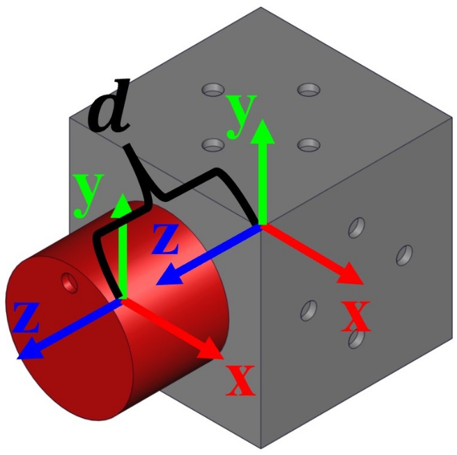
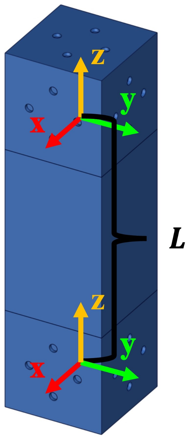
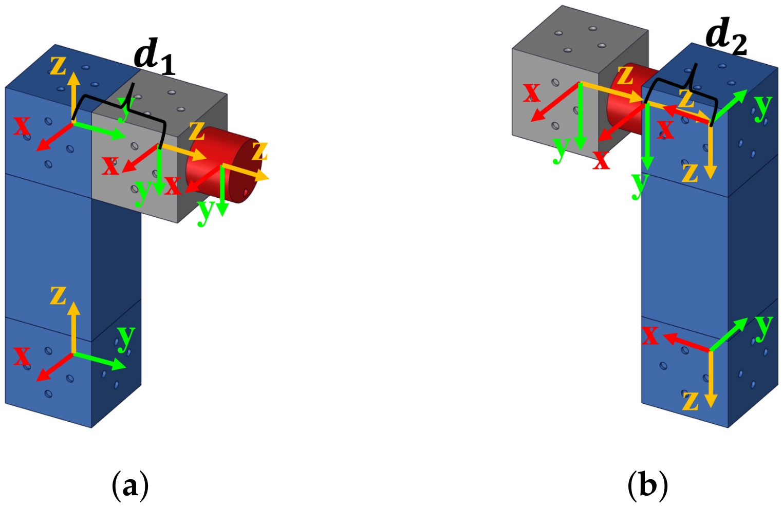
4.2. The Fixed Kinematic Transformation of Link Modules

For the link module (as shown in Figure 7), the fixed kinematic transformation between the two coordinate frames is fixed, which is determined by the length of the link module. As the two coordinate frames on the link modules, i.e., the input and output frames, are parallel to each other, the fixed kinematic transformation of link modules is given by:
T L = T L ( 0 ) = 1 0 0 0 0 1 0 0 0 0 1 L 0 0 0 1
where T L ( 0 ) is the initial pose of the output coordinate frame with respect to the input coordinate frame of the link module, in which L is the distance from the origin of the input coordinate frame to the origin of the output coordinate frame of the link module (as shown in Figure 7).

4.3. The Fixed Kinematic Transformation between Two Assembled Modules

When two robot modules are assembled together, the kinematic transformation between the modules needs to be determined, which can be described by the fixed kinematic transformation from the output coordinate frame of the proceeding module to the input coordinate frame of the succeeding module. It is given by:
T A = R p 0 1 SE ( 3 )
For the rotation matrix R SO ( 3 ) , its first, second, and third column are all unit vectors, denoted by e x , e y , e z . If two columns of R are known, the last column can be calculated by:
e x = e y × e z e y = e z × e x e z = e x × e y
To compute the fixed kinematic transformation between two assembled robot modules T A , two general assembly modes, i.e., the link module being the proceeding module (as shown in Figure 8a) and the joint module being the proceeding module (as shown in Figure 8b), are discussed.
For a link-joint module assembly, as shown in Figure 8a, the fixed kinematic transformation ( T A ) from the link’s output frame to the joint’s input frame is computed based on the port vectors of these two adjacent modules. Let P 1 = ( p 11 , p 12 ) and P 2 = ( p 21 , p 22 ) be the port vectors of the link module and joint module, respectively. The first parameter of the link’s port vector p 11 { ± x , ± y , + z } can be employed to determine the position vector p R 3 . If p 11 is ± x , then p = ( ± d 1 , 0 , 0 ) T ; if it is ± y , then p = ( 0 , ± d 1 , 0 ) T ; if it is + z , then p = ( 0 , 0 , d 1 ) T . In order to compute the orientation matrix R SO ( 3 ) , a computation algorithm is formulated as follows. Each parameter of a port vector is converted to a unit vector, such that if p i j ( i = 1 , 2 ; j = 1 , 2 ) is ± x , ± y , or ± z , then p i j will be converted to ( ± 1 , 0 , 0 ) , ( 0 , ± 1 , 0 ) , or ( 0 , 0 , ± 1 ) , respectively, denoted by p i j . Based on the kinematic relationship between the output port vector of the link module and the input port vector of the joint module, we have:
R p 21 p 22 p 21 × p 22 = p 11 p 12 p 11 × p 12
Therefore, the orientation matrix R is given by:
R = p 11 p 12 p 11 × p 12 p 21 p 22 p 21 × p 22 1
For example, P 1 = ( + y , z ) , P 2 = ( z , y ) (as shown in Figure 8), and we have:
p = ( 0 , d 1 , 0 ) T
R = 0 0 1 1 0 0 0 1 0 0 0 1 0 1 0 1 0 0 1 = 1 0 0 0 0 1 0 1 0
T A = 1 0 0 0 0 0 1 d 1 0 1 0 0 0 0 0 1
For a joint-link module assembly, as shown in Figure 8b, the fixed kinematic transformation ( T A ) from the joint’s output frame to the link’s input frame is computed based on the port vectors of these two adjacent modules. Let P 1 = ( p 11 , p 12 ) = ( + z , + y ) and P 2 = ( p 21 , p 22 ) be the port vectors of the joint module and link module, respectively. As with the link-joint module assembly, p 11 determines the position vector p . The computation algorithm of rotation matrix R is also the same. For example, P 1 = ( + z , + y ) , P 2 = ( + x , + z ) (as shown in Figure 8), and we have:
p = ( 0 , 0 , d 2 ) T
R = 0 0 1 0 1 0 1 0 0 1 0 0 0 0 1 0 1 0 1 = 0 1 0 0 0 1 1 0 0
T A = 0 1 0 0 0 0 1 0 1 0 0 d 2 0 0 0 1

4.4. Automatic Kinematic Modeling Based on AAM

Using the local frame representation of the POE formula, the forward kinematics of a serial-type MRR configuration can be expressed in the following form:
T 0 , n ( q ) = T 0 , 1 ( 0 ) e ξ ^ 1 q 1 T 1 , 2 ( 0 ) e ξ ^ 2 q 2 T n 1 , n ( 0 ) e ξ ^ n q n
where T 0 , n ( q ) is the pose of the end-effector relative to the base frame, q i ( i = 1 , 2 , n ) is the angle of the ith joint, ξ = ( v , ω ) is the twist of joint i expressed in frame i, and T i 1 , i ( 0 ) is the initial pose of the ith module relative to the ( i 1 ) th module, which is determined by the fixed kinematic transformation between two assembled modules and the initial poses of the two modules.
For example, the kinematics of an MRR with two robot modules (as shown in Figure 9) is:
T 0 , 2 ( q ) = T 0 , 1 ( 0 ) e ξ ^ 1 q 1 T 1 , 2 ( 0 )
in which,
T 0 , 1 ( 0 ) = T J ( 0 ) = 1 0 0 0 0 1 0 0 0 0 1 d 0 0 0 1 T 1 , 2 ( 0 ) = T A T L ( 0 ) = 0 1 0 0 0 0 1 0 1 0 0 d 2 0 0 0 1 1 0 0 0 0 1 0 0 0 0 1 L 0 0 0 1
For a branch-type MRR configuration with m branches, the kinematics is given by:
T ( q 1 , q 2 , , q n ) = T 0 , n = T 0 , n 1 ( 1 ) T 0 , n 2 ( 2 ) T 0 , n m ( m )
Once the AAM of an MRR assembly configuration is specified, its kinematic model can be automatically generated based on Equation (18) or (20). The kinematic modeling algorithm is given in Algorithm 1.
Algorithm 1 The Kinematics of MRRs
Input: AAM ( A A ); Joint angles q ;
Output: The pose of the end-effectors relative to the base frame, T 0 , n
1: Extract the last row of A A as M l and delete the last row of A A , then set all the non-zero entries to 1 to get the adjacency matrix;
2: Calculate the path matrix P ( G ) ;
3: Modify the path matrix ( P M ( G ) ) by using the vertices’ subscript to replace the non-zero entries and then deleting the zero entries;
4: According to P ( G ) , compute the module kinematics set, termed T m o d u l e ;
5: for  i = 1 to row of P M ( G )  do
6:      T 0 , n ( i ) = T m o d u l e ( i , 1 ) ;
7: for  i = 1 to row of P M ( G )  do
8:     for  j = 1 to column of P M ( G ) -1 do
9:          Δ = P M ( i , j + 1 ) P M ( i , j )
10:         Get the pair of port vectors P 1 = A A ( P M ( i , j ) + Δ , P M ( i , j ) ) , P 2 = A A ( P M ( i , j ) , P M ( i , j ) + Δ ) to compute the fixed kinematic transformation between the two assembled modules ( T A i , j );
11:          T 0 , n ( i ) = T 0 , n ( i ) T A i , j T m o d u l e ( i , j + 1 ) ;
12: return  T 0 , n

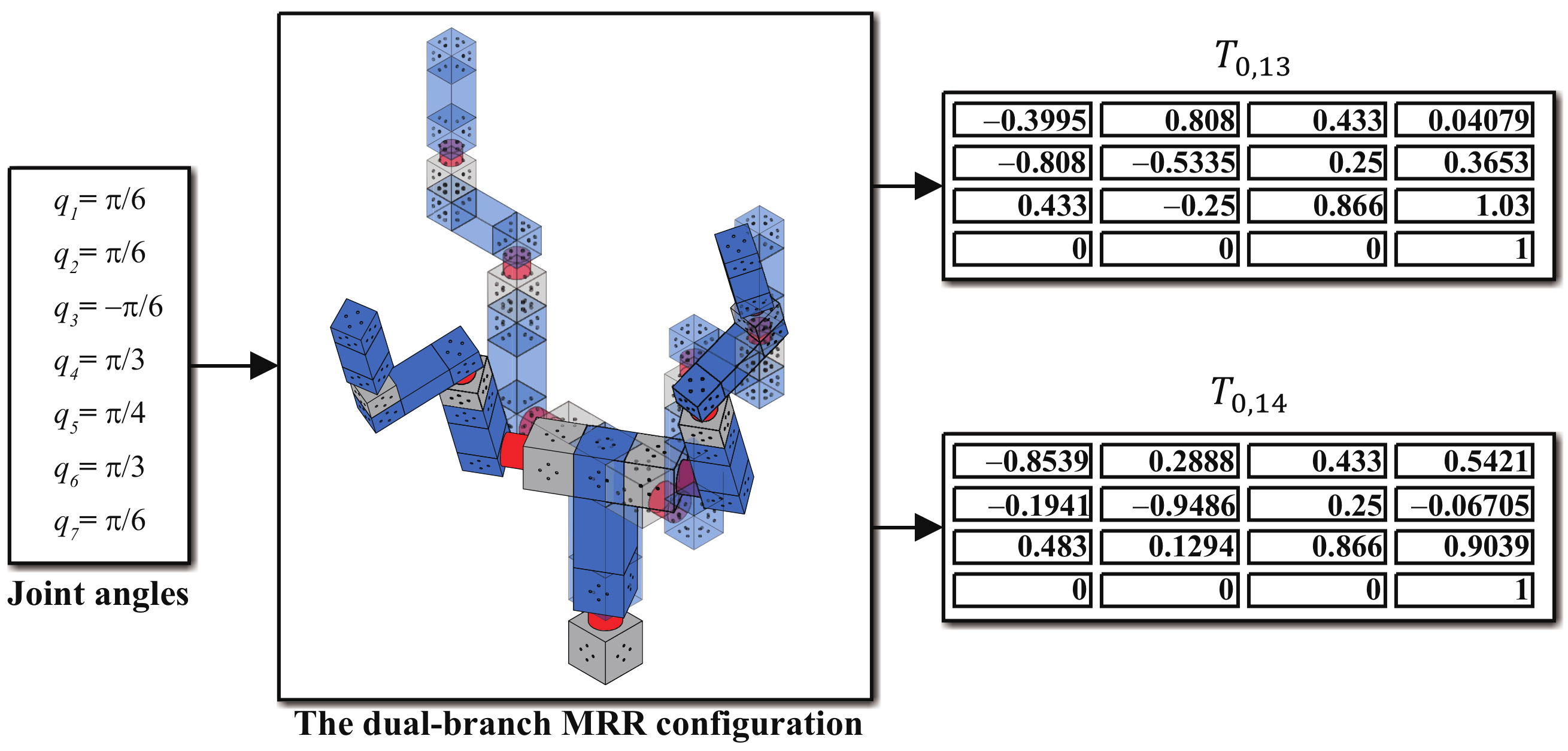
5. Simulation and Results

With the configuration-independent kinematic modeling algorithm, the kinematic model of an MRR can be automatically generated from its AAM, which is verified through the following simulation example. An MRR configuration and its AG are given in Figure 10.
The AAM ( A t ) of this dual-branch MRR assembly configuration is given by:
A t = a 1 , 1 a 1 , 2 a 1 , 14 a 2 , 1 a 2 , 2 a 2 , 14 a 15 , 1 a 15 , 2 a 15 , 14
in which the entries that are non-zero in A t are listed in Table 1.
According to Algorithm 1, the path matrix ( P ( G ) ) and the kinematics ( T ( q 1 , q 2 , , q n ) ) of this MRR configuration are obtained:
P ( G ) = 1 1 1 0 1 0 1 0 1 0 1 0 1 0 1 1 0 1 0 1 0 1 0 1 0 1 0 1
T ( q 1 , q 2 , , q n ) = T 0 , n = T 0 , 13 T 0 , 14
in which,
T 0 , 13 = T 0 , 1 ( 0 ) e ξ ^ 1 q 1 T 1 , 2 ( 0 ) T 2 , 3 ( 0 ) e ξ ^ 2 q 2 T 3 , 5 ( 0 ) T 5 , 7 ( 0 ) e ξ ^ 4 q 4 T 7 , 9 ( 0 ) T 9 , 11 ( 0 ) e ξ ^ 6 q 6 T 11 , 13 ( 0 ) T 0 , 14 = T 0 , 1 ( 0 ) e ξ ^ 1 q 1 T 1 , 2 ( 0 ) T 2 , 4 ( 0 ) e ξ ^ 3 q 3 T 4 , 6 ( 0 ) T 6 , 8 ( 0 ) e ξ ^ 5 q 5 T 8 , 10 ( 0 ) T 10 , 12 ( 0 ) e ξ ^ 7 q 7 T 12 , 14 ( 0 )
and T i , j ( i = 0 , 1 , , 12 ; j = 1 , 2 , , 14 ) are listed in Table 2.
Figure 11 shows the robot configuration with the joint angles:
q = { π 6 , π 6 , π 6 , π 3 , π 4 , π 3 , π 6 }
Substituting the joint angle values into Equation (23), the poses of the two end-effectors relative to the base frame are obtained as follows:
T 0 , 13 = 0.3995 0.8080 0.4330 0.04079 0.8080 0.5335 0.2500 0.3653 0.4330 0.2500 0.8660 1.03 0 0 0 1 T 0 , 14 = 0.8539 0.2888 0.4330 0.5421 0.1941 0.9486 0.2500 0.06705 0.4830 0.1294 0.8660 0.9039 0 0 0 1
To verify the proposed algorithm, the 3D modules are established in SOLIDWORKS, including three types of link modules and three types of joint modules. According to these modules, a dual-branch MRR is assembled. Then, the SOLIDWORKS model imported into MATLAB, and the multibody module is employed to verify the proposed algorithms. The simulation results are shown in Figure 12, which are the same as the results computed by the algorithm.

6. Conclusions

This paper investigates the assembly configuration representation and kinematic modeling issues for a Modular Reconfigurable Robot (MRR). By abstracting the commonly used robot modules from the existing MRRs, two types of robot modules, i.e., revolute joint modules and rigid link modules, with cuboid shapes are considered. An Assembly Graph (AG) is defined to represent the topological structure of an MRR configuration, in which all robot modules are treated as vertices, while their connecting interfaces are treated as edges. To mathematically represent all possible assembly configurations of an MRR, an Assembly Adjacency Matrix (AAM) is proposed. Owing to the unique treatment of joint modules in AG and AAM, the local frame representation of the POE formula can be directly applied to each of the joint modules, which is configuration-independent. Utilizing the AAM of an MRR configuration, the forward kinematic model of an MRR configuration is automatically generated. The effectiveness of the proposed assembly configuration representation method and kinematic modeling algorithm are verified through a simulation example.

Author Contributions

Conceptualization, T.Z. and G.Y.; methodology, T.Z.; software, T.Z.; validation, T.Z.; formal analysis, T.Z. and G.Y.; investigation, T.Z.; resources, G.Y., C.-Y.C., C.W., C.Z., S.C. and Z.F.; data curation, T.Z. and Q.D.; writing—original draft preparation, T.Z.; writing—review and editing, T.Z., Q.D. and G.Y.; visualization, T.Z. and Q.D.; supervision, G.Y. and C.Z.; project administration, G.Y., C.-Y.C., C.W., C.Z., S.C. and Z.F. All authors have read and agreed to the published version of the manuscript.

Funding

This research was funded by the National Natural Science Foundation of China, grant number 92048201; the Joint Funds of the National Natural Science Foundation of China, grant number U20A20282; the Major Program of Natural Science Foundation of Zhejiang Province, grant number LD22E050007; and the Major Special Projects of the Plan “Science and Technology Innovation 2025” in Ningbo, grant number 2018B10058.

Institutional Review Board Statement

Not applicable.

Informed Consent Statement

Not applicable.

Conflicts of Interest

The authors declare no conflict of interest.

Abbreviations

The following abbreviations are used in this manuscript:
MRRModular Reconfigurable Robot
AGAssembly Graph
AAMAssembly Adjacency Matrix
POEProduct of Exponentials
EAMExtended Adjacency Matrix
D-HDenavit–Hartenberg

References

  1. Althoff, M.; Giusti, A.; Liu, S.B.; Pereira, A. Effortless creation of safe robots from modules through self-programming and self-verification. Sci. Robot. 2019, 4, eaaw1924. [Google Scholar] [CrossRef] [PubMed]
  2. Kelmar, L.; Khosla, P. Automatic generation of kinematics for a reconfigurable modular manipulator system. In Proceedings of the 1988 IEEE International Conference on Robotics and Automation, Philadelphia, PA, USA, 24–29 April 1988; Volume 2, pp. 663–668. [Google Scholar] [CrossRef]
  3. Paredis, C.; Brown, H.; Khosla, P. A rapidly deployable manipulator system. Proc. IEEE Int. Conf. Robot. Autom. 1996, 2, 1434–1439. [Google Scholar] [CrossRef]
  4. Patel, H.; Singh, C.; Liu, G. Safe robot operation alongside humans using spring-assisted modular and reconfigurable robot. In Proceedings of the 2017 IEEE International Conference on Mechatronics and Automation (ICMA), Takamatsu, Japan, 6–9 August 2017; pp. 787–792. [Google Scholar] [CrossRef]
  5. Singh, C.; Liu, G. On Task-Specific Redundant Actuation of Spring-Assisted Modular and Reconfigurable Robot. In Proceedings of the 2020 IEEE International Conference on Mechatronics and Automation (ICMA), Beijing, China, 13–16 October 2020; pp. 1191–1196. [Google Scholar] [CrossRef]
  6. Liu, C.; Yim, M. A Quadratic Programming Approach to Modular Robot Control and Motion Planning. In Proceedings of the 2020 Fourth IEEE International Conference on Robotic Computing (IRC), Taichung, Taiwan, 9–11 November 2020; pp. 1–8. [Google Scholar] [CrossRef]
  7. Liu, C.; Yu, S.; Yim, M. A Fast Configuration Space Algorithm for Variable Topology Truss Modular Robots. In Proceedings of the 2020 IEEE International Conference on Robotics and Automation (ICRA), Paris, France, 31 May–31 August 2020; pp. 8260–8266. [Google Scholar] [CrossRef]
  8. Zhao, S.; Zhao, J.; Sui, D.; Wang, T.; Zheng, T.; Zhao, C.; Zhu, Y. Modular Robotic Limbs for Astronaut Activities Assistance. Sensors 2021, 21, 6305. [Google Scholar] [CrossRef] [PubMed]
  9. Memar, A.H.; Esfahani, E.T. Modeling and Dynamic Parameter Identification of the SCHUNK Powerball Robotic Arm. In Proceedings of the ASME 2015 International Design Engineering Technical Conferences and Computers and Information in Engineering Conference, Boston, MA, USA, 2–5 August 2015; Volume 5C: 39th Mechanisms and Robotics Conference. [Google Scholar] [CrossRef] [Green Version]
  10. Dogra, A.; Padhee, S.S.; Singla, E. Optimal Architecture Planning of Modules for Reconfigurable Manipulators. Robotica 2020, 1–15. [Google Scholar] [CrossRef]
  11. Dogra, A.; Sekhar Padhee, S.; Singla, E. An Optimal Architectural Design for Unconventional Modular Reconfigurable Manipulation System. J. Mech. Des. 2020, 143, 063303. [Google Scholar] [CrossRef]
  12. Yun, A.; Moon, D.; Ha, J.; Kang, S.; Lee, W. ModMan: An Advanced Reconfigurable Manipulator System with Genderless Connector and Automatic Kinematic Modeling Algorithm. IEEE Robot. Autom. Lett. 2020, 5, 4225–4232. [Google Scholar] [CrossRef]
  13. Romiti, E.; Malzahn, J.; Kashiri, N.; Iacobelli, F.; Ruzzon, M.; Laurenzi, A.; Hoffman, E.M.; Muratore, L.; Margan, A.; Baccelliere, L.; et al. Toward a Plug-and-Work Reconfigurable Cobot. IEEE/ASME Trans. Mechatron. 2021, 1–13. [Google Scholar] [CrossRef]
  14. Chen, I.M.; Yang, G. Configuration independent kinematics for modular robots. Proc. IEEE Int. Conf. Robot. Autom. 1996, 2, 1440–1445. [Google Scholar] [CrossRef]
  15. Zhao, J.; Tang, S.F.; Zhu, Y.H.; Cui, X.D. Topological description method of UBot self-reconfigurable robot. Harbin Gongye Daxue Xuebao/J. Harbin Inst. Technol. 2011, 43, 46–49+55. [Google Scholar]
  16. Nainer, C.; Feder, M.; Giusti, A. Automatic Generation of Kinematics and Dynamics Model Descriptions for Modular Reconfigurable Robot Manipulators. In Proceedings of the 2021 IEEE 17th International Conference on Automation Science and Engineering (CASE), Lyon, France, 23–27 August 2021; pp. 45–52. [Google Scholar] [CrossRef]
  17. Honerkamp, D.; Welschehold, T.; Valada, A. Learning Kinematic Feasibility for Mobile Manipulation Through Deep Reinforcement Learning. IEEE Robot. Autom. Lett. 2021, 6, 6289–6296. [Google Scholar] [CrossRef]
  18. Mahkam, N.; Özcan, O. A framework for dynamic modeling of legged modular miniature robots with soft backbones. Robot. Auton. Syst. 2021, 144, 103841. [Google Scholar] [CrossRef]
  19. Dalla Libera, A.; Castaman, N.; Ghidoni, S.; Carli, R. Autonomous Learning of the Robot Kinematic Model. IEEE Trans. Robot. 2021, 37, 877–892. [Google Scholar] [CrossRef]
  20. Denavit, J.; Hartenberg, R.S. A Kinematic Notation for Lower-Pair Mechanisms. J. Appl. Mech. 1955, 22, 215–221. [Google Scholar] [CrossRef]
  21. Chen, I.M. Theory and Applications of Modular Reconfigurable Robotic System. Ph.D. Thesis, California Institute of Technology, Pasadena, CA, USA, 1994. [Google Scholar]
  22. Yang, G.; Chen, I.M. A novel kinematic calibration algorithm for reconfigurable robotic systems. Proc. Int. Conf. Robot. Autom. 1997, 4, 3197–3202. [Google Scholar] [CrossRef]
  23. Chen, I.M.; Yang, G. Automatic Model Generation for Modular Reconfigurable Robot Dynamics. J. Dyn. Syst. Meas. Control 1998, 120, 346. [Google Scholar] [CrossRef]
  24. Yang, G. Kinematics, Dynamics, Calibration, and Configuration Optimization of Modular Reconfigurable Robots. Ph.D. Thesis, School of Mechanical and Production Engineering, Nanyang Technological University, Singapore, 1999. [Google Scholar]
  25. Brockett, R.W. Robotic manipulators and the product of exponentials formula. In Mathematical Theory of Networks and Systems; Fuhrmann, P.A., Ed.; Springer: Berlin/Heidelberg, Germany, 1984; pp. 120–129. [Google Scholar]
  26. Park, F.C.; Kim, B.; Jang, C.; Hong, J. Geometric Algorithms for Robot Dynamics: A Tutorial Review. Appl. Mech. Rev. 2018, 70, 010803. [Google Scholar] [CrossRef]
  27. Kollmorgen. Available online: https://www.kollmorgen.com/sites/default/files/public_downloads/RGM_UserManual_PDF.pdf (accessed on 15 December 2021).
Figure 1. The internal architecture of a revolute joint module.
Symmetry 14 00433 g001
Figure 2. Revolute joint modules. (a) A commercialized revolute “I” type joint module. (b) A commercialized “T” type revolute joint module [27]. (c) The abstracted revolute joint module.
Symmetry 14 00433 g002
Figure 3. Link modules. (a) The “H” type link module. (b) The “L” type link module. (c) The abstracted link module.
Symmetry 14 00433 g003
Figure 4. The Assembly Graph (AG) of an MRR assembly configuration. (a) The assembly configuration of an MRR. (b) The AG of the MRR assembly configuration.
Symmetry 14 00433 g004
Figure 5. Port vector in a link module.
Symmetry 14 00433 g005
Figure 6. The abstracted revolute joint module with a cube-cylinder geometry and multiple connecting ports.
Symmetry 14 00433 g006
Figure 7. The abstracted link module with a cuboid geometry and multiple connecting ports.
Symmetry 14 00433 g007
Figure 8. Two module assemblies. (a) A link-joint module assembly. (b) A joint-link module assembly.
Symmetry 14 00433 g008
Figure 9. An MRR with two robot modules.
Symmetry 14 00433 g009
Figure 10. A 7-DOF dual-branch MRR. (a) The MRR configuration. (b) The AG of the MRR.
Symmetry 14 00433 g010
Figure 11. The resulting configuration of the dual-branch MRR with given joint angles.
Symmetry 14 00433 g011
Figure 12. The simulation results of a dual-branch MRR configuration.
Symmetry 14 00433 g012
Table 1. The non-zero entries in A t .
ColumnValue
1 a 2 , 1 = ( + z , + y ) , a 15 , 1 = J 3
2 a 1 , 2 = ( z , + y ) , a 3 , 2 = ( + y , z ) , a 4 , 2 = ( y , + z ) , a 15 , 2 = L 3
3 a 2 , 3 = ( z , + y ) , a 5 , 3 = ( + z , + y ) , a 15 , 3 = J 3
4 a 2 , 4 = ( z , + y ) , a 6 , 4 = ( + z , + y ) , a 15 , 4 = J 3
5 a 3 , 5 = ( + y , z ) , a 7 , 5 = ( + z , x ) , a 15 , 5 = L 2
6 a 4 , 6 = ( + y , + z ) , a 8 , 6 = ( + z , + y ) , a 15 , 6 = L 2
7 a 5 , 7 = ( z , + y ) , a 9 , 7 = ( + z , + y ) , a 15 , 7 = J 2
8 a 6 , 8 = ( z , + y ) , a 10 , 8 = ( + z , + y ) , a 15 , 8 = J 2
9 a 7 , 9 = ( + x , y ) , a 11 , 9 = ( x , + z ) , a 15 , 9 = L 1
10 a 8 , 10 = ( + x , z ) , a 12 , 10 = ( x , + y ) , a 15 , 10 = L 1
11 a 9 , 11 = ( z , + y ) , a 13 , 11 = ( + z , + y ) , a 15 , 11 = J 1
12 a 10 , 12 = ( z , + y ) , a 14 , 12 = ( + z , + y ) , a 15 , 12 = J 1
13 a 11 , 13 = ( z , + x ) , a 15 , 13 = L 1
14 a 12 , 14 = ( z , y ) , a 15 , 14 = L 1
Table 2. The value of T i , j .
Value
T 0 , 1 T J 3 ( 0 )
T 1 , 2 T A 1 , 2 T L 3 ( 0 )
T 2 , 3 T A 2 , 3 T J 3 ( 0 )
T 2 , 4 T A 2 , 4 T J 3 ( 0 )
T 3 , 5 T A 3 , 5 T L 2 ( 0 )
T 4 , 6 T A 4 , 6 T L 2 ( 0 )
T 5 , 7 T A 5 , 7 T J 2 ( 0 )
T 6 , 8 T A 6 , 8 T J 2 ( 0 )
T 7 , 9 T A 7 , 9 T L 1 ( 0 )
T 8 , 10 T A 8 , 10 T L 1 ( 0 )
T 9 , 11 T A 9 , 11 T J 1 ( 0 )
T 10 , 12 T A 10 , 12 T J 1 ( 0 )
T 11 , 13 T A 11 , 13 T L 1 ( 0 )
T 12 , 14 T A 12 , 14 T L 1 ( 0 )
Publisher’s Note: MDPI stays neutral with regard to jurisdictional claims in published maps and institutional affiliations.

