
Application of Lie Symmetry to a Mathematical Model that Describes a Cancer Sub-Network


Department of Mathematics, University of Zululand, Private Bag X1001, Kwadlangezwa 3886, Kwazulu Natal, South Africa
Symmetry 2022, 14(2), 400; https://doi.org/10.3390/sym14020400
Submission received: 3 December 2021
/
Revised: 24 January 2022
/
Accepted: 10 February 2022
/
Published: 17 February 2022
(This article belongs to the Special Issue Symmetry in Functional Equations and Analytic Inequalities II)
Abstract
:In this paper, a mathematical model of a cancer sub-network is analysed from the view point of Lie symmetry methods. This model discusses a human cancer cell which is developed due to the dysfunction of some genes at the R-checkpoint during the cell cycle. The primary purpose of this paper is to apply the techniques of Lie symmetry to the model and present some approximated solutions for the three-dimensional system of first-order ordinary differential equations describing a cancer sub-network. The result shows that the phosphatase gene (Cdc25A) regulates the cyclin-dependent kinases inhibitor (). Furthermore, this research discovered that the activity that reverses the inhibitory effects on cell cycle progression at the R-checkpoint initiates a pathway.
1. Introduction
Over the last two decades, researchers have developed mathematical models to understand the dynamic mechanisms of the cell cycle [1,2,3,4]. In [5,6,7], scholars used non-linear differential equations to model cell cycle mutations as limit cycles. The R-checkpoint, according to Pardee, represents a unique switch between the quiescent and proliferative phases of normal cells [7]. Researchers further highlighted the importance of the R-checkpoint in preventing malignant transformation [8]. As a result, if a cell has damaged DNA or has not grown properly, the cell cycle is said to be stalled [2,9,10]. In particular, genes such as phosphatase Cdc25A, cyclins , cyclin-dependent kinases , retinoblastoma protein , cyclin-dependent kinases inhibitor , and transcriptional factors (E2F, C-Myc) are the most significant control regulators [2,9,10,11].
A mathematical model can be defined as the representation and development of a previously investigated process. This insight has led to the creation of mathematical forms that represent real-world scenarios. This will make it easier to comprehend the phenomenon that has been observed. The Lie symmetry technique and numerical analyses provide understanding, responses, and useful guidance in analysing the formulated mathematical model.
In this study, a mathematical model of a cancer sub-network is analysed from the view point of Lie symmetry. This technique is indeed a powerful tool for solving non-linear differential equations. The Cancer Sub-Network model is governed by the following three-dimensional system of first-order non-linear differential equations [10]:
where the dependent variables and parameters are described in the table below (Table 1). The terms , , and refer to protein degradation caused by ubiquitin-proteasomes with the fixed rate coefficients , , and [10]. The inhibition nature of cell to and of to are represented by and , respectively.
The rest of the paper is organised as follows. In Section 2, a realistic background of the fundamental theories of Lie symmetry are presented. A simplified and parametrised form of the Cancer Sub-Network model is developed in Section 3. Lie symmetry analysis of the model is performed in Section 4. The numerical solutions are performed and presented graphically in Section 5. Finally, a discussion and concluding remarks are provided in Section 6.
2. Preliminaries on Lie Symmetry Method
In this Section, a summary of the Lie symmetry analysis to solve a system of differential equations is provided. The method comprises the tools that are needed in this study. Firstly, the mathematical concept of symmetry is enlightened. Secondly, the overall properties of groups are given and extended to the Lie groups. Several textbooks are available in the literature. Furthermore, numerous research articles are published on the theory of the Lie symmetry technique for solving ordinary differential equations (ODEs) as well as partial differential equations (PDEs).
In accordance with the theory of Lie symmetry, the given three-dimensional system of the first-order differential equation is as follows:
which admits the following Lie group of one-parameter transformations (a):
with the infinitesimal Lie operators below:
The group transformations , , , and are obtained by solving the following Lie equations [8]:
with the initial conditions:
The first extension of the Lie operators above is defined as follows:
where
with representing the total differential operator, described as follows:
The infinitesimal transformation obtained will be used to solve the following equation:
Equation (4) will provide a set of new independent variable r, and dependent variables u, v, and w, which can be used to transform the non-linear system (1) into a linear system.
Theorem 1.
A function is invariant under the prolonged group G if and only if [14]:
where
is the kth extension of the Lie operator of G.
Theorem 2.
Considering that the Lie groups of point transformations related to a given differential equation involve n independent variables and m dependent variables [16,17], let:
be a group of transformations in the space of the variables [17,18]. Moreover, let the following equation:
be a solution for the equation . A Lie group of transformations of the form (5) admitted by has the two corresponding properties below [15,17]:
- A transformation of the group maps any solution of into another solution of ;
- A transformation of the group leaves invariant, supposing that reads the same in terms of the variables and in terms of the transformed variables .
3. Simplification and Parametrisation Form of Model (1)
In this Section, a reduction of the number of parameters from the original model is performed. As a result, a cosmetic simplification of the non-linear system (1) is achieved below.
By letting:
The left-hand side of the model Equation (1) becomes:
4. Lie Symmetry Analysis of the Model (9)
By applying Equations (2) and (3) into the Non-dimensional model Equation (9), we obtain the following:
The substitution of extended infinitesimal transformations into Equation (3) gives the following equations:
where
Special solutions are needed since it is generally challenging to solve the non-linear system (12). In the case of , , , , the non-linear Equation (12) is reduced as follows:
Taking the partial derivative of Equation (15) with respect to yields to the following second-order partial differential equation:
which implies that:
with the and constants of integration. The substitution of Equation (16) into (13)–(15) gives the following:
Twice partially differentiating Equation (18) with respect to gives:
Hence,
Since Equation (20) depends on all values of and , we get the following:
Hence,
From (19), we obtain:
Hence,
Therefore, the infinitesimals transformations are provided as follows:
It is important to note that these infinitesimal transformations are not unique. However, there exists an infinite set of infinitesimal transformations. Therefore, Equation (2) becomes:
Hence, the following Lie generators are found:
By computing the Lie bracket, we obtain the given commutator table (Table 2):
By setting the constant of integration to , , , , . Equation (21) becomes:
Hence, we have the following equations:
The solution of Equation (22) is given by:
The special case is given by:
Substituting back to Equation (6), we obtain the following:
5. Numerical Solutions
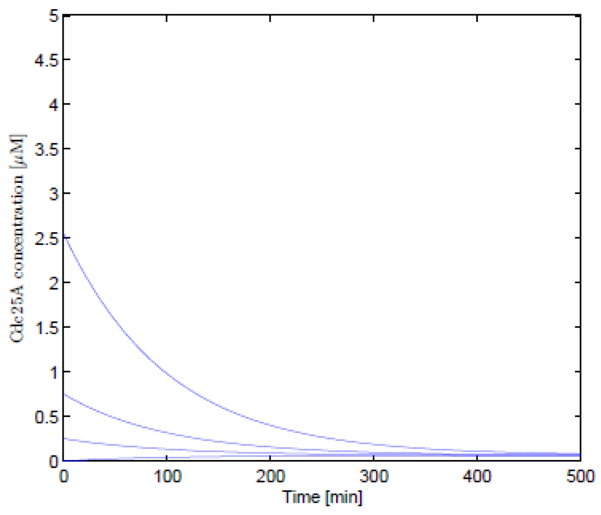
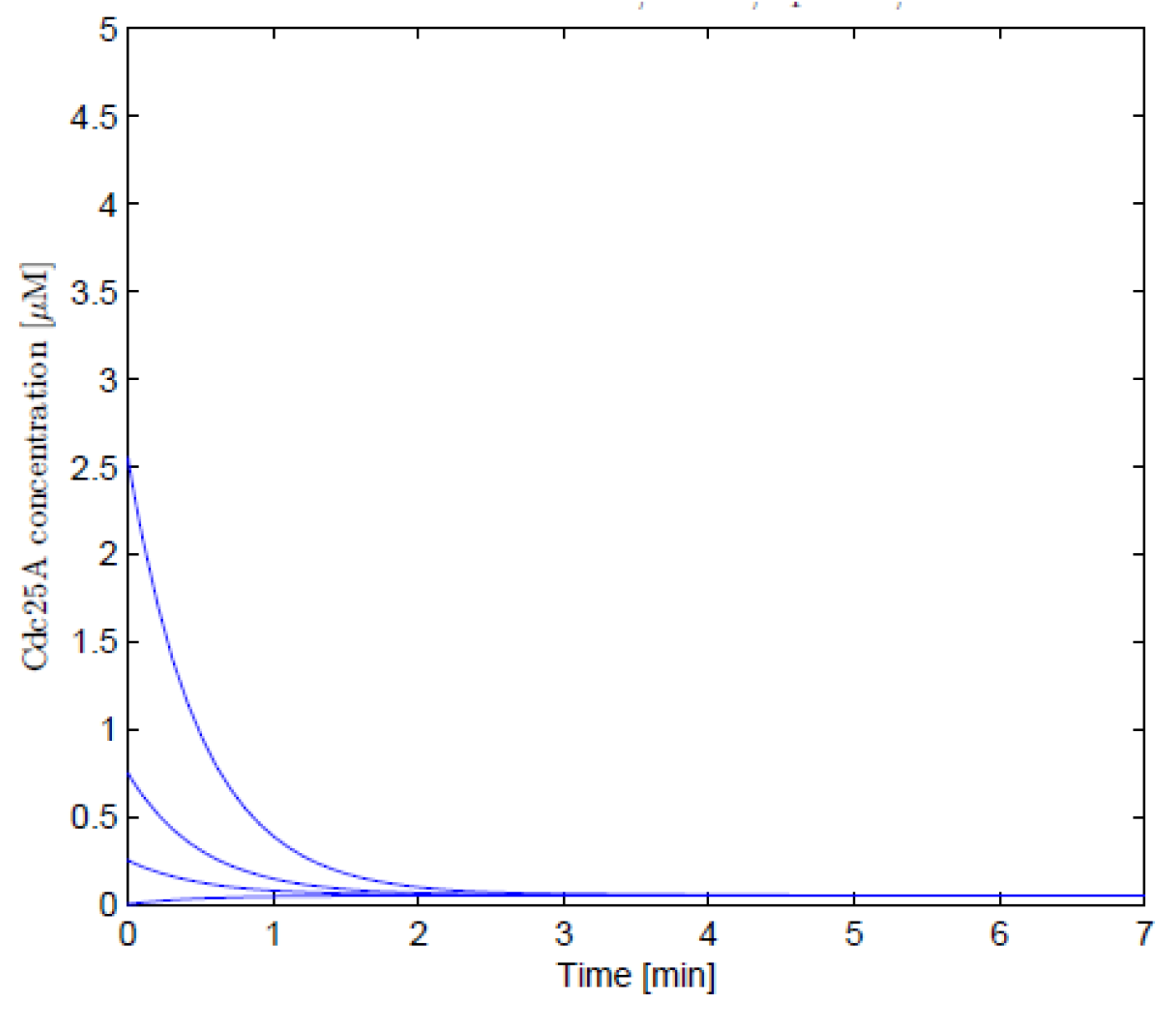
As illustrated in the graphs below, the numerical solutions for non-linear differential equations were obtained using the Matlab software. Figure 1 and Figure 2 show the numerical solutions for Equations (1) and (23), respectively. Numerical results obtained before and after using the Lie symmetry techniques on the Cancer Sub-Network model were found to be consistent. The parameters chosen were , , , and the effect of the synthesis rate of Cdc25A has initial values of , , , ; . The simulation results are in line with Aguda and Tang’s findings [2], which show that phosphatase gene (Cdc25A) activity increases in lockstep with cyclin-dependent kinase inhibitor () levels.
6. Conclusions
The cancer sub-network revealed in this research is significantly simplified in comparison to what is known as the molecular and gene interactions of the oncogene and the tumour-suppressor gene. On the other hand, applying Lie symmetry analysis and computationally modelling the full cancer network during the cell cycle phase is challenging. To represent the cancer network, we started with a simple model that encapsulated the network’s key features. This model can be updated in the future to make it more realistic.
In this paper, the Lie symmetry technique was applied to obtain a modified, local, one-parameter infinitesimal transformation. Furthermore, Lie operators and Lie algebra were discovered to be useful in obtaining approximated solutions for the non-linear cancer network model. The results of the numerical simulations were found to be consistent with the findings of Aguda and Tang [2]. The model simulation revealed that when the complex’s degradation rate is less than 0.001 min (all other parameters remaining constant), the subnetwork generates a peak value for the phosphatase gene (Cdc25A) activity.
Funding
The University of Zululand’s research office provided financial support for this study.
Acknowledgments
The University of Zululand’s research office provided financial support for this study. The author would like to thank the reviewers for their insightful comments and suggestions, which significantly improved the manuscript.
Conflicts of Interest
The author declares no conflict of interest.
References
- Aguda, B.D. A Quantitative Analysis of the Kinetics of the G2 DNA Damage Checkpoint System. Proc. Natl. Acad. Sci. USA 1999, 96, 11352–11357. [Google Scholar] [CrossRef] [PubMed] [Green Version]
- Aguda, B.D.; Tang, T. The Kinetic Origins of the Restriction Point in the Mammalian Cell Cycle. Cell Prolif. 1999, 32, 321–335. [Google Scholar] [CrossRef] [PubMed]
- Gardner, T.S.; Dolnik, M.; Collins, J.J. A Theory for Controlling Cell Cycle Dynamics using a Reversibly Binding Inhibitor. Proc. Natl. Acad. Sci. USA 1998, 95, 14190–14195. [Google Scholar] [CrossRef] [PubMed] [Green Version]
- Thron, C.D. Bistable Biochemical Switching and the Control of the Events of the Cell Cycle. Oncogene 1997, 15, 317–325. [Google Scholar] [CrossRef] [PubMed] [Green Version]
- Goldbeter, A. A Minimal Cascade Model for the Mitotic Oscillators Involving Cyclin and Cdc2 Kinases. Proc. Natl. Acad. Sci. USA 1991, 88, 9107–9111. [Google Scholar] [CrossRef] [PubMed] [Green Version]
- Norel, R.; Agur, Z. A Model for the Adjustment of the Mitotic Clock by Cyclin and MPF Levels. Science 1991, 251, 1076–1078. [Google Scholar] [CrossRef] [PubMed]
- Zhilin, Q.; Weiss, J.N.; Maclellan, W.R. Regulation of the Mammalian Cell Cycle: A Model of the G1-to-S Transition. Am. J. Physiol.–Cell Physiol. 2002, 284, C349–C364. [Google Scholar]
- Zondi, P.L.; Matadi, M.B. Lie group theoretic approach of one-dimensional Black-Scholes equation. Aust. J. Math. Anal. Appl. 2021, 18, 1–19. [Google Scholar]
- Aguda, B.D. Analysis of Cancer Gene Networks in Cell Proliferation and Death; Information and Communication Technologies for Health: New York, NY, USA, 2008. [Google Scholar]
- Yibeltal, B.N. Identifying and Modelling the Dynamics of a Core Cancer Sub-Network; University of KwaZulu Natal Press: Pietermaritzburg, South Africa, 2011; pp. 50–52. [Google Scholar]
- Jun-ya, K. Induction of S Phase by G1 Regulatory Factors. Front. Biosci. 1999, 4, 787–792. [Google Scholar]
- Pardee, A.B. A Restriction Point for Control of Normal Animal Cell Proliferation. Proc. Natl. Acad. Sci. USA 1974, 71, 1286–1290. [Google Scholar] [CrossRef] [PubMed] [Green Version]
- Pardee, A.B. G1 Events and Regulation of Cell Proliferation. Science 1989, 246, 603–608. [Google Scholar] [CrossRef] [PubMed]
- Masebe, T.P. A Lie Symmetry Analysis of the Black-Scholes Merton Finance Model through Modified Local One-Parameter Transformations; University of South Africa Press: Unisa, South Africa, 2014; pp. 37–80. [Google Scholar]
- Matadi, M.B. Jacoby last multiplier and group theoretic approaches to a model describing breast cancer stem cells. Commun. Math. Biol. Neurosci. 2021, 2021, 85. [Google Scholar]
- Matadi, M.B. Lie Symmetry Analysis Of Early Carcinogenesis Model. Appl. Math. E-Notes 2018, 18, 238–249. [Google Scholar]
- Oliveri, F. Lie Symmetries of Differential Equations: Classical results and recent contributions. Symmetry 2010, 2, 658–706. [Google Scholar] [CrossRef] [Green Version]
- Matadi, M.B. The Conservative Form of Tuberculosis Model with Demography. Far East J. Math. Sci. 2017, 102, 2403–2416. [Google Scholar] [CrossRef]
Figure 1.
The numerical results of Equation (1).
Figure 1.
The numerical results of Equation (1).

Figure 2.
The numerical results of Equation (23).
Figure 2.
The numerical results of Equation (23).


Table 1.
Description of variables and parameters.
| Variable and Parameter | Description | References | |
|---|---|---|---|
| 1 | concentration of gene Cdc25A | [1,11] | |
| 2 | concentration of gene | [1,2] | |
| 3 | concentration of gene | [1,12] | |
| 4 | constitutive protein expressions of Cdc25A | [7,9] | |
| 5 | constitutive protein expressions of | [2,9] | |
| 6 | mitogenic signal stimulation | [2,3] | |
| 7 | a | activation efficiency of by | [2,6] |
| 8 | b | activation efficiency of by | [2,10] |
| 9 | c | inhibition coefficients of to | [1,2,13] |
| 10 | d | inhibition coefficients of to | [2,13] |
| 11 | production rates of to | [2,9] | |
| 12 | production rates of to | [2,9] |
Table 2.
The commutator table of the infinitesimal generator.
| 0 | 0 | 0 | 0 | |||
| 0 | 0 | 0 | 0 | 0 | ||
| 0 | 0 | 0 | 0 | 0 | ||
| 0 | 0 | 0 | 0 | − | 0 | |
| 0 | 0 | 0 | 0 | 0 | ||
| 0 | 0 | 0 | 0 | 0 | 0 |
Publisher’s Note: MDPI stays neutral with regard to jurisdictional claims in published maps and institutional affiliations. |
© 2022 by the author. Licensee MDPI, Basel, Switzerland. This article is an open access article distributed under the terms and conditions of the Creative Commons Attribution (CC BY) license (https://creativecommons.org/licenses/by/4.0/).
Share and Cite
MDPI and ACS Style
Matadi, M.B. Application of Lie Symmetry to a Mathematical Model that Describes a Cancer Sub-Network. Symmetry 2022, 14, 400. https://doi.org/10.3390/sym14020400
AMA Style
Matadi MB. Application of Lie Symmetry to a Mathematical Model that Describes a Cancer Sub-Network. Symmetry. 2022; 14(2):400. https://doi.org/10.3390/sym14020400
Chicago/Turabian StyleMatadi, Maba Boniface. 2022. "Application of Lie Symmetry to a Mathematical Model that Describes a Cancer Sub-Network" Symmetry 14, no. 2: 400. https://doi.org/10.3390/sym14020400
Note that from the first issue of 2016, this journal uses article numbers instead of page numbers. See further details here.