Article

A Software Reliability Model with Dependent Failure and Optimal Release Time

1
Department of Computer Science and Statistics, Chosun University, 309 Pilmun-daero, Dong-gu, Gwangju 61452, Korea
2
Department of Industrial and Systems Engineering, Rutgers University, 96 Frelinghuysen Road, Piscataway, NJ 08855-8018, USA
*
Author to whom correspondence should be addressed.
Symmetry 2022, 14(2), 343; https://doi.org/10.3390/sym14020343
Submission received: 31 December 2021 / Revised: 15 January 2022 / Accepted: 7 February 2022 / Published: 8 February 2022
(This article belongs to the Topic Applied Metaheuristic Computing)

Abstract

:
In the past, because computer programs were restricted to perform only simple functions, the dependence on software was not large, resulting in relatively small losses after a failure. However, with the development of the software market, the dependence on software has increased considerably, and software failures can cause significant social and economic losses. Software reliability studies were previously conducted under the assumption that software failures occur independently. However, as software systems become more complex and extremely large, software failures are becoming frequently interdependent. Therefore, in this study, a software reliability model is developed under the assumption that software failures occur in a dependent manner. We derive the software reliability model through the number of software failure and fault detection rate assuming point symmetry. The proposed model proves good performance compared with 21 previously developed software reliability models using three datasets and 11 criteria. In addition, to find the optimal release time, a cost model using the developed software reliability model was presented. To determine this release time, four parameters constituting the software reliability model were changed by 10%. By comparing the change in the cost model and the optimal release time, it was found that parameter b had the greatest influence.

1. Introduction

Software, one of the main components of a computer, plays an important role in the operation of physical devices. Software was originally developed with the ability to perform extremely small or simple functions. Currently, however, embedded systems that perform multiple functions are being developed. With the rapid development of the software market, technology has also developed, and software is now being used in all fields. Recently, the Internet of Things (IoT) based on the combination of various software, has been commercialized. Furthermore, AIoT (Artificial Intelligence of Things) combined AI (Artificial Intelligence) with IoT (Intelligence of Things) is developing [1]. It means that software has become a very important part not only in the industrial field but also in our daily life.
A software failure is caused by various faults (coding or system errors, etc.). In the past, software failures caused relatively small losses because the degree of software dependence was not as large. However, in today’s world, the degree of dependence on software is extremely high, and thus software failures can cause significant social and economic losses. Therefore, we measured the software reliability, which indicates the ability of a software program to avoid failure for a set period of time and refers to how long the software can be used without such a failure.
Early research on software reliability was conducted based on the assumption that software failures occur independently. Goel and Okumoto proposed the GO model, which is the most basic non-homogeneous Poisson process (NHPP) software reliability growth model [2]. The Hossain, Dahiya, Goel and Okumoto (HDGO) model further extended the GO model [3]. Yamada et al., Ohba, and Zhang et al. [4,5,6] proposed an NHPP S-shaped curve model in which the cumulative number of software failures increases to the S curve. In addition, Yamada et al. [7] proposed a new model in which the test effort invested during phase was reflected in the software reliability model. It is a model that reflects even the resources consumed for testing in the previously developed model. Furthermore, Yamada et al. [8] developed a software reliability model with a constant fault detection rate of b ( t ) = b , assuming incomplete debugging, in which faults detected during the test phase were corrected and removed.
The model developed by extending the above approach involved a generalized incomplete debugging-error detection rate model. Here, the fault detection rate b ( t ) of the model is not a constant but rather a different function [9,10,11,12,13,14]. It started from the software error causing the failure being immediately eliminated and so a new error can be generated [9]. It progressed to that during the fault removal process, whether the fault is removed successfully or not, new faults are generated with a constant probability [13,14]. In addition, because the operating environment of the software is operated differently for each software program, a comparison is difficult to achieve. Therefore, in [15,16,17], a software reliability model was developed considering uncertain factors in the operating environment. Currently, research using non-parametric methods such as deep learning or machine learning is also being conducted [18,19,20,21].
Recently, finding the most optimal model for reliability prediction is an important concern. Through combination of analytic hierarchy method (AHP), hesitant fuzzy (HF) sets and techniques for order of preference by similarity to ideal solution (TOPSIS), Sahu et al., Ogundoyin et al., and Rafi et al. [22,23,24] found the most optimal software reliability model.
However, software failures often occur in a dependent manner because the developed software is composed of extremely complex structures [25]. Here, the dependent failure means that one failure affects other failures or increases the failure probability of other equipment [26,27]. There are two main types of dependent failure. A common cause failure is when several pieces of software fail simultaneously due to a common cause, and a cascading failure is a case in which a part of the system fails and affects other software as well. A software reliability model assuming a dependent failure was developed from the number of software failures and the fault detection rate, which have a dependency relationship in a software reliability model assuming incomplete debugging [28]. In addition, Lee et al. [29] presented a model that assumes that if past software failures are not corrected well, they will continue to have an effect.
In this study, a new software reliability model is developed under the assumption that software failures occur in a dependent manner. It is suitable for a general environment. We show the superiority of the newly developed dependent software reliability model through a comparison under various criteria. In addition, determining the optimal release time of the developed software is also important. If the test period is long, the software will be reliable, but the software development cost will increase. If the test period is short, the reliability of the product may decrease. Therefore, it is important to find a balance between time to market and minimum cost taking into account the installation costs, test costs, and error removal costs, etc. We propose a cost model that combines the proposal software reliability model and the cost coefficient [30,31,32,33]. In addition, among the various parameters of the proposed model, we propose a parameter that has a significant influence on predicting the number of cumulative failures through a variation in the cost model for changes in the parameters [34,35]. Section 2 introduces a new dependent software reliability model and its mathematical derivation. Section 3 introduces the data and criteria, as well as numerical results. Section 4 describes the optimal release time, and finally, in Section 5, we present our conclusions

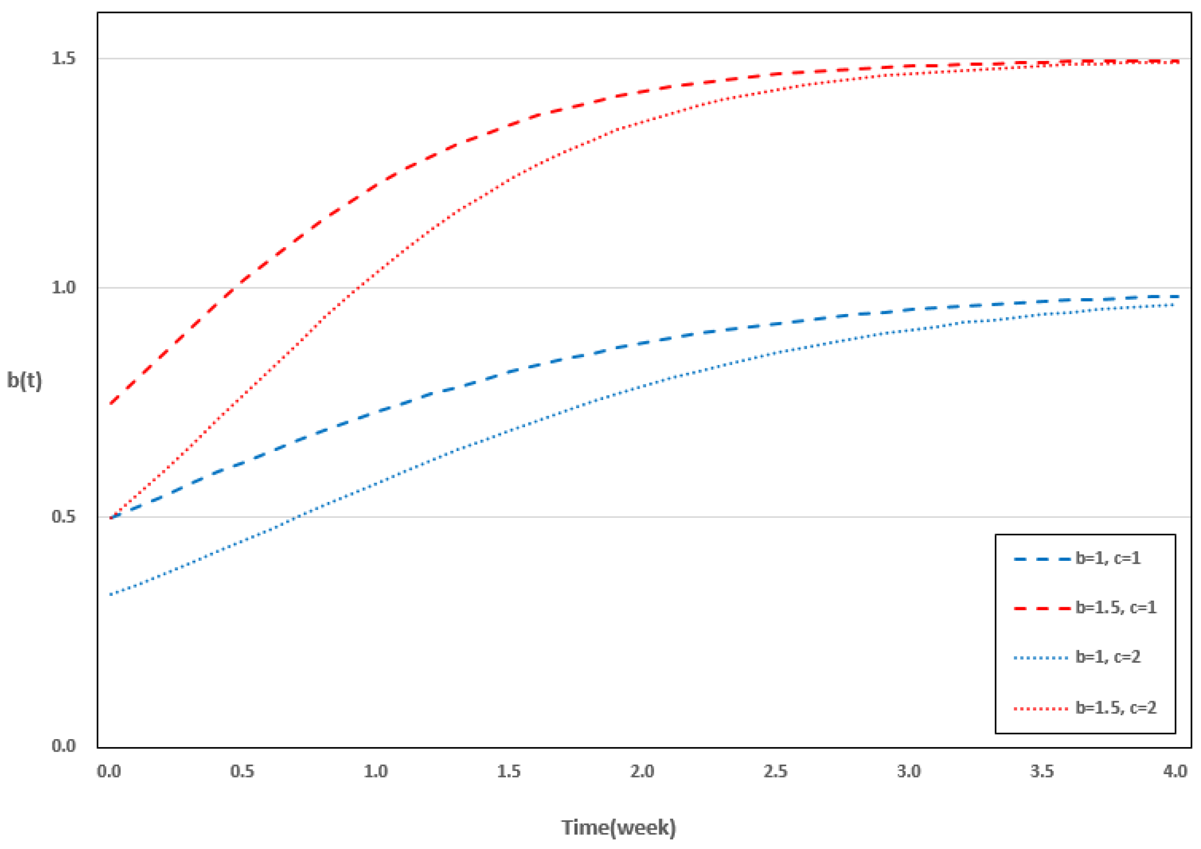
2. New Dependent Software Reliability Model

Software reliability refers to the probability that the software will not fail a system for a certain period of time under certain conditions. In other words, it evaluates “how long the software can be used without failure”. The reliability function used to evaluate this is as follows:
R ( t ) = P ( T > t ) = t f ( u ) d u
This denotes the probability of the software operating without failure over a specific time t . Here, the probability density function f ( t ) assumes the software failure time or lifetime as a random variable T . When measuring reliability function R ( t ) , it is assumed that it follows an exponential distribution with parameter λ . In addition, it is assumed that the number of failures occurring in given unit time is a Poisson distribution with parameter λ . When λ is a constant, it is the most basic form, and is called a homogeneous Poisson process. Extending this process, many researchers adapt a model where λ is an intensity function λ ( t ) that changes with time rather than a single constant by setting λ as a non-homogeneous Poisson process(NHPP) rather than as a homogeneous Poisson process.
Pr { N ( t ) = n } = { m ( t ) } n n ! e m ( t ) , n = 0 , 1 , 2 , ,   t 0
In Equation (2), N ( t ) is the Poisson probability density function with the time dependent parameter m ( t ) . The m ( t ) is a mean value function which is the integral of λ ( t ) from 0 to t in Equation (3). The λ ( t ) is the intensity function indicating the number of instantaneous failures at time t .
m ( t ) = E [ N ( t ) ] = 0 t λ ( s ) d s
A general class of NHPP software reliability models was proposed by Equation (9) to summarize the existing NHPP models as follows:
d m ( t ) d t = b ( t ) [ a ( t ) m ( t ) ]
where, the m ( t ) is calculated using the relationship between the number of failures a ( t ) at each time point and a fault detection rate b ( t ) assuming point symmetry in Equation (4). Various software reliability models have been developed based on the assumption that software failures occur independently.
However, software failures occur not only independently but also dependently. If the failure is not completely fixed, it will continue to affect the next failure. In addition, as the system becomes more complex, the relationship between failure and failure also shows the dependent relationship because of the dependent combination of several software. Therefore, in this study, we assume that failure is dependent on other failures. The mean value function m ( t ) based on NHPP software reliability model using the differential equation is as follows:
d m ( t ) d t = b ( t ) [ a ( t ) m ( t ) ] m ( t )
In Equation (5), the m ( t ) is multiplied once more to assume that the failure occurring from 0 to t affects another failure. We assume:
a ( t ) = a ( 1 + α t ) ,   b ( t ) = b 1 + c e b t
where, a ( t ) is the number of software failures at each time point and b ( t ) is the fault detection rate. Parameter a is the expected number of faults, α is the increasing rate of the number of faults, b is the shape parameter, and c is the scale parameter. When time t changes, the change according to the values of parameters b and c in the fault detection rate b ( t ) are as shown in Figure 1. When b is 1 , it is blue, and when it is 1.5 , it is red. In addition, when c is 1 , it is a dashed line, and when it is 2 , it is a dotted line. It can be seen that the larger b is, the larger the b ( t ) is.
When solving the differential equation by substituting a ( t ) and b ( t ) for m ( t ) in Equations (5) and (6), we obtain Equation (7):
m ( t ) = ( c + e b t ) a ( c + e b t c ) a α t e a α L i 2 ( e b t + c c ) b ( c + e b t ) a ( c + e b t c ) a α t e a α L i 2 ( e b t + c c ) b b e b t c + e b t d t + C
where L i s ( x ) = n = 1 x n n s is a polylogarithm when s = 2 . At this time, α = 0 in a ( t ) .
m ( t ) = h ( c + e b t ) a h [ 0 t ( e b x + c ) a b e b x c + e b x d x ] + ( 1 + c ) a
where h is the number of initial failures. In Equation (8), 0 t ( e b x + c ) a b e b x c + e b t d x is calculated through an integration using substitution. When u = c + b e b x and d u = b e b x d x , it is the same as in Equation (9).
0 t ( e b x + c ) a b e b x c + e b t d x = c + b c + b e b t u a u d u = c + b c + b e b t u a 1 d u = u a a = ( c + e b t ) a a
Substituting the result of the substitution integration into Equation (8), the final m ( t ) is given by Equation (10).
m ( t ) = a 1 + a h ( 1 + c c + e b t ) a
This can be presented as a general model of a dependent failure occurrence in the software reliability model. When t = 0 , m ( t ) is m ( 0 ) = a h / ( a + h ) . Table 1 shows the value of m ( t ) of the existing software reliability model and the model proposed in this study. From models 19–22, it is assumed that a failure occurs in a dependent manner.

3. Numerical Examples

3.1. Data Information

Datasets 1 and 2 are derived from the online communication system (OCS) of ABC Software Co. and uses data accumulated over a 12 -week period. Datasets 1 and 2 show that the cumulative number of failures at t = 1 ,   2 ,   ,   12 is 14 ,   17 ,   ,   81 , and 11 ,   17 ,   ,   81 , respectively [14]. Dataset 3 is the test data of a medical record system consisting of 188 software titles and data for one of three releases. It shows that the cumulative number of failures is 90 ,   107 ,   ,   204 for t = 1 ,   2 ,   ,   17 , respectively [36]. Table 2 shows the accumulated failure data for datasets 1, 2, and 3. We compare the fit between the software reliability models with two failure datasets obtained from OCS and one dataset from Lee et al. [29], which showed good performance as the dependent models (DPF).

3.2. Criteria

This study compares various independent and dependent software reliability models and the proposed model introduced Table 1 using 11 criteria. Based on the difference between the actual observed value and the estimated value, we would like to find a better model by comparing it with criteria reflecting the number of parameters used in each model.
First, the mean squared error (MSE) is defined as the sum of squares of the distance between the estimated value and the actual value when considering the number of parameters and the number of observations [37].
MSE = i = 1 n ( m ^ ( t i ) y i ) 2 n m
where m ^ ( t i ) is the estimated value of the model m ( t ) , y i is the actual observed value, n is the number of observations, and m is the number of parameters in each model.
Second, the mean absolute error (MAE) defines the difference between the estimated number of failures and the actual value considering the number of parameters and the number of observations as the sum of the absolute values [38].
MAE = i = 1 n | m ^ ( t i ) y i | n m
Third, Adj _ R 2 is the modified coefficient of determination of the regression equation and determines how much explanatory power it has in consideration of the number of parameters [39].
R 2 = 1 i = 1 n ( m ^ ( t i ) y i ) 2 i = 1 n ( y i y i ¯ ) 2 ,   Adj _ R 2 = 1 ( 1 R 2 ) ( n 1 ) n m 1
Fourth, the predictive ratio risk (PRR) is obtained by dividing the distance from the actual value to the estimated value by the estimated value in relation to the model estimation [40].
PRR = i = 1 n ( m ^ ( t i ) y i m ^ ( t i ) ) 2
Fifth, the predictive power (PP) is obtained by dividing the distance from the actual value to the estimated value by the actual value [41].
PP = i = 1 n ( m ^ ( t i ) y i y i ) 2
Sixth, Akaike’s information criterion (AIC) was used to compare likelihood function maximization. This is applied to maximize the Kullback–Leibler level between the probability distribution of the model and the data [42].
AIC = 2 log L + 2 m L = i = 1 n ( m ( t i ) m ( t i 1 ) ) y i y i 1 ( y i y i 1 ) ! e ( m ( t i ) m ( t i 1 ) ) l o g L = i = 1 n { ( y i y i 1 ) ln ( m ( t i ) m ( t i 1 ) ) ( m ( t i ) m ( t i 1 ) ) ln ( ( y i y i 1 ) ! ) }
Seventh, the predicted relative variation (PRV) is the standard deviation of the prediction bias and is defined as [43]
PRV = i = 1 n ( y i m ^ ( t i ) B i a s ) 2 n 1
Here, the bias is i = 1 n [ m ^ ( t i ) y i n ] .
The root mean square prediction error (RMSPE) can estimate the closeness with which the model predicts the observation [44]:
RMSPE = V a r i a n c e 2 + B i a s 2
Ninth, the mean error of prediction (MEOP) sums the absolute value of the deviation between the actual data and the estimated curve and is defined as [38]
MEOP = i = 1 n | m ^ ( t i ) y i | n m + 1
Tenth, the Theil statistic (TS) is the average percentage of deviation over all periods with regard to the actual values. The closer the Theil statistic is to zero, the better the prediction capability of the model. This is defined as [45]
TS = 100 i = 1 n ( y i m ^ ( t i ) ) 2 i = 1 n y i 2 %
Eleventh, it takes into account the tradeoff between the uncertainty in the model and the number of parameters in the model by slightly increasing the penalty each time parameters are added to the model when the sample is considerably small [46].
PC = ( n m 2 ) log ( i = 1 n ( m ^ ( t i ) y i ) 2 n ) + m ( n 1 n m )
Based on the above criteria, we compared the proposed model with the existing NHPP software reliability model. When Adj _ R 2 is closer to 1 , and the other 10 criteria are closer to 0 , it indicates a better fit. Using R and MATLAB, the parameters of each model were estimated through the LSE method, and the goodness of fit is calculated to compare the superiority. This is a method of estimating parameters through the difference between the model in Table 1 and the actual number of failures in Table 2, and follows LSE = t = 1 n ( y t m ( t ) ) 2 [47].

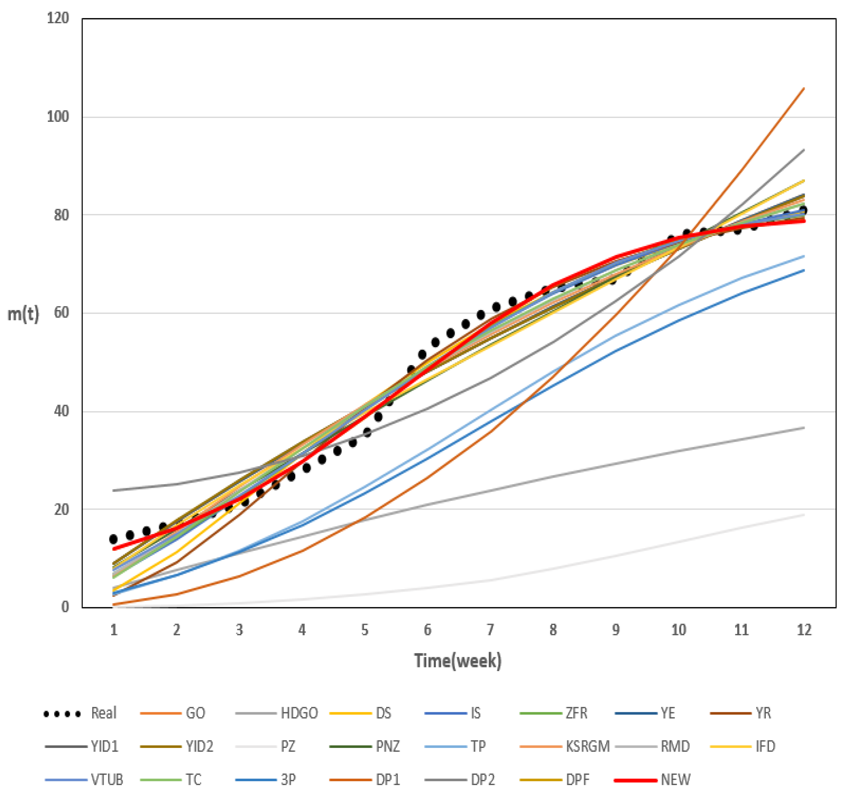
3.3. Results of Dataset 1

Table 3 shows the estimated values for the parameters of each model obtained using dataset 1. Each parameter of the proposed model is represented by a ^ = 80.0907 , b ^ = 0.07231 , c ^ = 15.9288 , and h ^ = 9.8182 . Figure 2 shows the result of calculating the estimated value of m ( t ) at each time point based on the cumulative number of failures at each time point in dataset 1 and each model equation. The black dotted line represents the actual data, and the dark red solid line represents the predicted failure value at each time point of the proposed model. Compared with other models, it shows the predicted value closest to the actual value.
Table 4 shows the results of calculating the criteria of each model using the parameters obtained through dataset 1. As a result, the values of MSE , MAE , PRR , PP , PRV , RMSPE , MEOP , TS , PC of the proposed model show the smallest values of 9.9274 , 3.2140 , 0.0647 , 0.0577 , 2.6866 , 2.6870 , 2.8569 , 4.6682 , and 13.0594 , respectively. The AIC shows the second smallest value at 73.4605 . In addition, Adj _ R 2 is 0.9821, which is the closest to 1 . The DPF model shows the highest value with AIC = 73.2850 , and the second highest result for the other criteria. The model with the third highest criterion is the Vtub model.

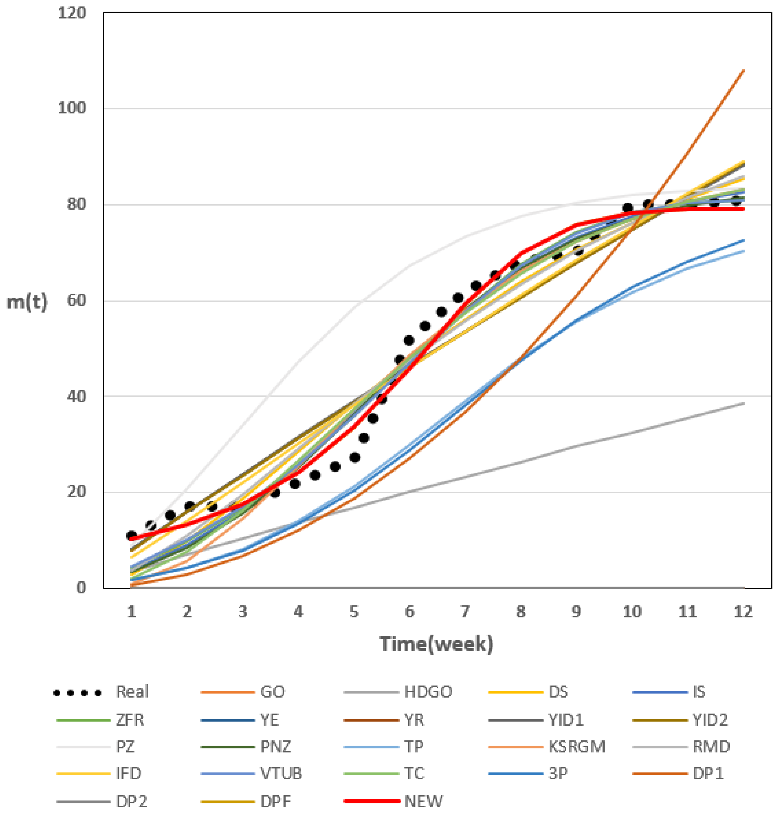
3.4. Results of Dataset 2

Table 5 shows the estimated values for the parameters of each model obtained using dataset 2. Each parameter of the proposed model is represented as a ^ = 79.1444 , b ^ = 0.2001 , c ^ = 72.3208 , and h ^ = 9.3327 . Figure 3 shows the results of calculating the estimated value of m ( t ) for each point in time based on the cumulative number of failures at each time point in dataset 2 and each model equation. Here, the black dotted line represents the actual data, whereas the dark red solid line represents the predicted failure value at each time point of the proposed model. Compared with the other models, the predicted value is closest to the actual value.
Table 6 shows the results of calculating the criteria of each model using the parameters obtained through dataset 2. As a result, the values of MSE , MAE , PRR , PP , AIC , PRV , RMSPE , MEOP , TS , and PC of the proposed model are 18.9722 , 4.3544 , 0.1615 , 0.1482 , 92.2155 , 3.7139 , 3.7145 , 3.8706 , 6.3751 , and 15.6500 , respectively, which show the smallest criteria. Adj _ R 2 is 0.9723 , which is the closest to 1. The model with the second highest criterion is DPF, and Vtub is the third best-fitting model.

3.5. Results of Dataset 3

Table 7 shows the estimated values for the parameters of each model obtained using dataset 3. Each parameter of the proposed model is represented through a ^ = 194.7684 , b ^ = 0.3062 , c ^ = 307.0805 , and h ^ = 135.5641 . Figure 4 shows the results of calculating the estimated value of m ( t ) at each point in time based on the number of cumulative failures at each time point in dataset 3 and for each model equation. The black dotted line indicates the actual data, and the dark red solid line is the predicted failure value at each time point for the proposed model. Compared with other models, the proposed model shows the predicted value closest to the actual value.
Table 8 shows the results of calculating the criteria of each model using the parameters obtained through dataset 3. As a result, MSE and PC of the proposed model show the smallest values of 26.8047 and 24.5551 , respectively, and Adj _ R 2 shows the closest value to 1 at 0.9765 . In addition, MAE , PRR , PP , PRV , RMSPE , MEOP , and TS are 4.9209 , 0.0096 , 0.0092 , 4.6668 , 4.6668 , 4.5694 , and 2.5484 , respectively, showing the second smallest values. Figure 4 shows the estimated failure values at each time point using the developed models. The Vtub model shows the most suitable criteria of 0.0094 , 0.0090 , 4.6356 , 4.6357 , and 2.5315 in PRR , PP , PRV , RMSPE , and TS , and DPF shows the most suitable criteria of 4.9195 and 4.5682 with MAE and MEOP . However, in calculating the AIC of the Vtub model, DPF, KSRGM, and the newly proposed model, a value indicating t = 14 is shown, indicating that the calculation is no longer being applied. In the process of calculating the AIC value, if there is no difference between the value at a specific point in time and the next point in time, the denominator is 0, so the AIC calculation can not be performed.

4. Optimal Release Time

When releasing software, it is very important that find the optimal release time. In order to find that, we need to find a time that minimizes the cost. We apply m ( t ) proposed in Section 2 to the cost model to find the optimal time point between time to market and the minimum cost. The optimal time is suggested based on the cost model that reflects the software installation cost, software test cost, operation cost, software removal cost, and risk cost when the software failure occurs. Figure 5 describes the software field environment from the software installation of the software cost model. The expected software cost model follows Equation (22) [30,31].
C ( T ) = C 0 + C 1 T + C 2 m ( T ) + C 3 ( 1 R ( x | T ) )
where C 0 is the installation cost for system testing, C 1 is the system test cost per unit time, C 2 is the error removal cost per unit time during the test phase, and C 3 is the penalty cost owing to a system failure. In addition, x represents the time the software was used. In addition, in the cost model equation, R ( x | T ) follows (23) [32,33].
R ( x | T ) = e [ m ( t + x ) m ( t ) ]
In this section, we propose a cost model using dataset 1 based on the proposed software reliability model and find the optimal time point between time to market and the minimum cost by changing the cost coefficients from C 0 to C 3 .

4.1. Results of the Optimal Release Time

For the parameters of the cost model, a ,   b ,   c ,   and   h calculated through numerical examples described in Section 3 were used. The cost coefficient of the cost model aims to find the optimal release time with the lowest cost by finding the optimal value through the changes in several values. The baseline value of the cost coefficient is as follows:
C 0 = 500 ,   C 1 = 20 ,   C 2 = 50 ,   C 3 = 5000 ,   x = 6
Here, baseline denotes to the reference value for confirming the change of the cost coefficient. The total cost value obtains as a reference value is 4888.856 , and the optimal release time T at this time is 18.3 . Table 9 changes the cost coefficient of each reference value, checks the minimum cost C ( T ) and optimal release time T * , and then checks the changing trend to find the most optimal release time T * . When x = 2 , the smallest total cost value obtains 4886.985 at T * = 18.2 . When x = 4 , the smallest total cost value shows 4888.735 at T * = 18.3 . When x = 6 , the smallest total cost value shows 4888.856 at T * = 18.3 . When x is 8 and 10 , the smallest total cost value shows 4888.863 at T * = 18.3 .
Here, C 0 is the setup cost, and as the value increases, the cost, which is directly proportional, increases as well; thus, the lower the setup cost is, the lower the cost. Table 10 compares the changes when the coefficients of are 300 , 500 , and 700 . It is found that the higher the value is, the higher the total cost value, whereas the optimal time does not change. Therefore, it appears that C 0 does not help determine the optimal release point. However, because the setup cost for a system stabilization is required, the appropriate C 0 cost coefficient is set to 500 . Figure 6 shows a graph of the results according to the change in C 0 .
Table 11 compares the changes when the coefficients of C 1 are 10 , 20 , and 30 . The results show that when C 1 is 10 , the total cost is the minimum at approximately 18.9 to 19.0 , and when C 1 is 20 , the minimum value is at 18.2 to 18.3 , and when it is 30 , the total cost shows the minimum value at approximately 17.8 to 17.9 . As the cost coefficient C 1 increases, the optimal release time is gradually pushed back. Figure 7 shows a graph of the results according to the changes in C 1 .
Table 12 compares the changes when the coefficients of C 2 are 30 , 40 , 50 , and 60 . It can be seen that the cost coefficient C 2 does not change from 18.2 to 18.3 at the optimal release time as the value changes. Figure 8 shows a graph of the results according to the change in C 2 .
Table 13 compares the changes when the coefficients of C 3 are 5000 , 7000 , 10,000 , and 15,000 . The results show that when C 3 is 5000 , the total cost is the minimum at approximately 18.2 to 18.3 ; when it is 7000 , it shows the minimum value at 18.5 to 18.6 ; when it is 10,000 , the total cost shows the minimum value at approximately 18.9 to 19.0 ; and when it is 15,000 , the total cost shows the minimum value at approximately 19.2 to 19.3 . This indicates that the optimal release time gradually increases as the cost coefficient C 3 increases. Figure 9 shows a graph of the results according to the changes in C 3 .

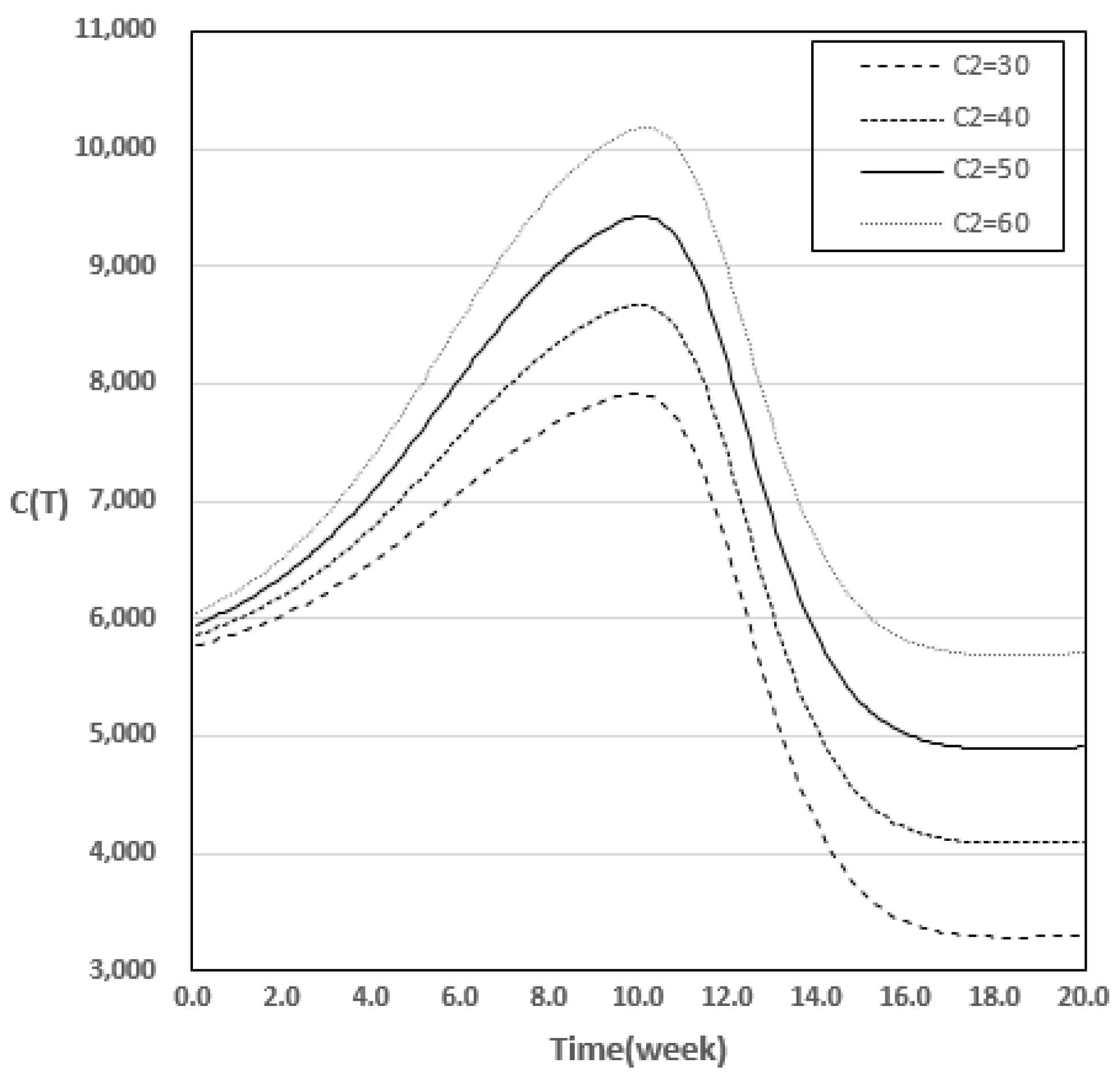
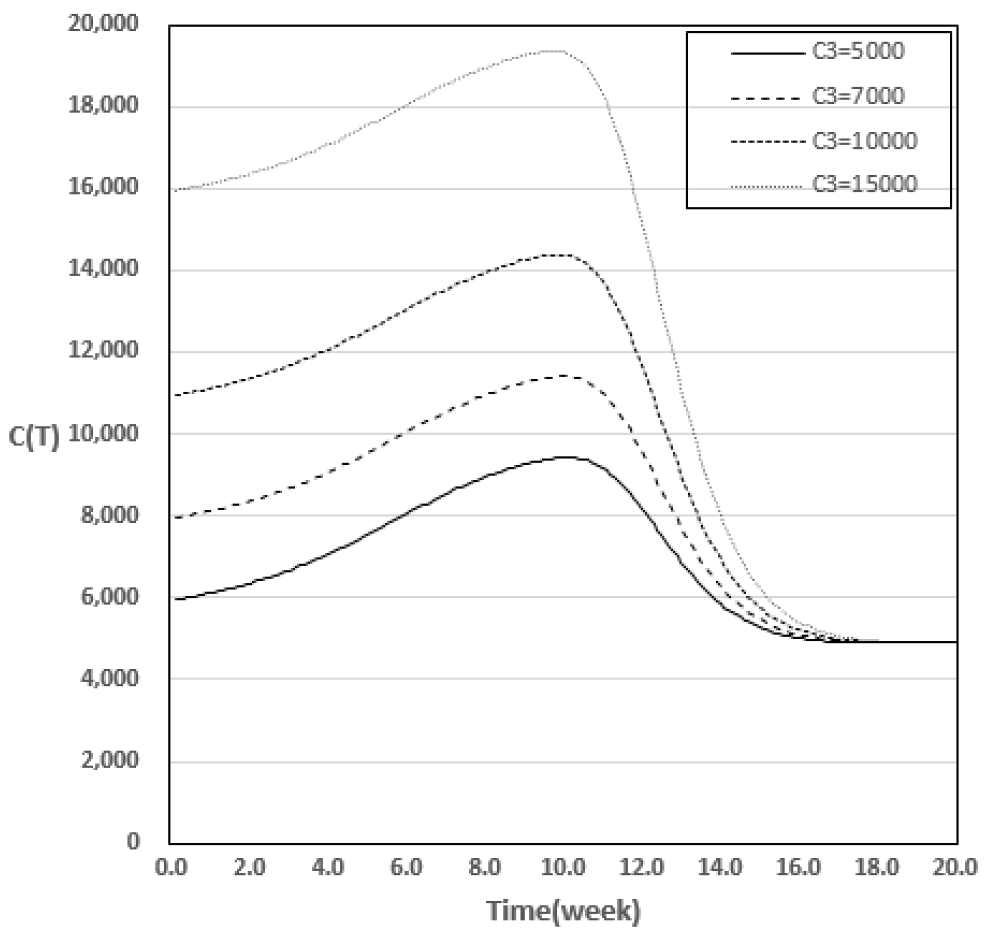
4.2. Results of Variation in Cost Model for Changes in Parameter

In this section, we check whether the optimal release time is affected by the change in the cost model according to the change in the parameters of the proposed model. The parameters a ,   b ,   c , and h of the proposed model are set at −20%, −10%, 0%, 10%, and 20%, respectively, in 10% increments, and the coefficient of the cost model is fixed at the baseline value in Section 4.1. Thus, the minimum cost value is calculated depending on changes in the parameters, and it derives appropriate release time. In Table 14, 0% is the same as the value suggested in Table 9 by substituting the parameter estimates described in Section 3 and the coefficient values of the cost model proposed in Section 4.
From Table 14 and Figure 10, Figure 11, Figure 12 and Figure 13, the value of the cost model C ( T ) increases as the change in parameter a increases, whereas the optimal release time T * decreases. As the values of parameters b and h increase, the cost model C ( T ) increases, and the release time T * is shown to decrease; in addition, it is found that the change in parameter h had a very slight effect on the optimal release time compared to parameter b . As the value of parameter c increases, the cost model C ( T ) and release time T * increase together. Based on this, it is found that parameter a had a very large minimum width of the cost model compared with the changes of the other parameters, and parameter b had the greatest influence on determining the optimal release time.

5. Conclusions

In this study, a new software reliability model was developed under the assumption that software failures occur in a dependent manner. We used three datasets for our evaluations. The first and second datasets showed the best fit, and the third dataset showed better results compared with many previously proposed models. The proposed model showed better results than DP1, DP2, and DPF, which are previously developed software-dependent failure occurrence models.
In addition, based on the proposed model, the optimal release time according to the change in the cost coefficient was suggested, and the total cost was analyzed accordingly. When the test cost was increased, the release time gradually increased, as did the overall cost; therefore, the optimal release time can be achieved when C 1 is 20. In the proposed model, fault detection rate b was found to be the most important parameter for determining the optimal release time.
In the past, studies were conducted by assuming independence in the case of software failures; however, in a real environment, the software execution environment is extremely diverse and complex. Therefore, it is necessary to develop a model that assumes a dependent failure occurrence and propose a model that considers the actual operating environment. We plan to conduct a study using machine learning and deep learning for the proposed software-dependent failure occurrence in the future work.

Author Contributions

Conceptualization, H.P.; Funding acquisition, I.H.C., K.Y.S.; Software, Y.S.K.; Writing—original draft, Y.S.K.; Writing—review and editing, K.Y.S., I.H.C. and H.P. All authors have read and agreed to the published version of the manuscript.

Funding

This research was supported by the Basic Science Research Program through the National Research Foundation of Korea (NRF) funded by the Ministry of Education (NRF-2018R1D1A1B07045734, NRF-2021R1F1A1048592, and NRF-2021R1I1A1A01059842).

Institutional Review Board Statement

Not required.

Informed Consent Statement

Not applicable.

Data Availability Statement

Data available in a publicly accessible repository.

Acknowledgments

This research was supported by the National Research Foundation of Korea. We are pleased to thank the Editor and the Referees for their useful suggestions.

Conflicts of Interest

The authors declare no conflict of interest.

References

  1. Wu, Y.C.; Wu, Y.J.; Wu, S.M. An outlook of a future smart city in Taiwan from post–internet of things to artificial intelligence internet of things. In Smart Cities: Issues and Challenges; Elsevier: Amsterdam, The Netherlands, 2019; pp. 263–282. [Google Scholar]
  2. Goel, A.L.; Okumoto, K. Time-dependent error-detection rate model for software reliability and other performance measures. IEEE Trans. Reliab. 1979, 28, 206–211. [Google Scholar] [CrossRef]
  3. Hossain, S.A.; Dahiya, R.C. Estimating the parameters of a non-homogeneous Poisson-process model for software reliability. IEEE Trans. Reliab. 1993, 42, 604–612. [Google Scholar] [CrossRef]
  4. Yamada, S.; Ohba, M.; Osaki, S. S-shaped reliability growth modeling for software fault detection. IEEE Trans. Reliab. 1983, 32, 475–484. [Google Scholar] [CrossRef]
  5. Ohba, M. Inflection S-shaped software reliability growth model. In Stochastic Models in Reliability Theory; Osaki, S., Hatoyama, Y., Eds.; Springer: Berlin, Germany, 1984; pp. 144–162. [Google Scholar]
  6. Zhang, X.M.; Teng, X.L.; Pham, H. Considering fault removal efficiency in software reliability assessment. IEEE Trans. Syst. Man Cybern. Part A-Syst. Hum. 2003, 33, 114–120. [Google Scholar] [CrossRef]
  7. Yamada, S.; Ohtera, H.; Narihisa, H. Software Reliability Growth Models with Testing-Effort. IEEE Trans. Reliab. 1986, 35, 19–23. [Google Scholar] [CrossRef]
  8. Yamada, S.; Tokuno, K.; Osaki, S. Imperfect debugging models with fault introduction rate for software reliability assessment. Int. J. Syst. Sci. 1992, 23, 2241–2252. [Google Scholar] [CrossRef]
  9. Pham, H.; Zhang, X. An NHPP software reliability models and its comparison. Int. J. Reliab. Qual. Saf. Eng. 1997, 4, 269–282. [Google Scholar] [CrossRef]
  10. Pham, H.; Nordmann, L.; Zhang, X. A general imperfect software debugging model with S-shaped fault detection rate. IEEE Trans. Reliab. 1999, 48, 169–175. [Google Scholar] [CrossRef]
  11. Teng, X.; Pham, H. A new methodology for predicting software reliability in the random field environments. IEEE Trans. Reliab. 2006, 55, 458–468. [Google Scholar] [CrossRef]
  12. Kapur, P.K.; Pham, H.; Anand, S.; Yadav, K. A unified approach for developing software reliability growth models in the presence of imperfect debugging and error generation. IEEE Trans. Reliab. 2011, 60, 331–340. [Google Scholar] [CrossRef]
  13. Roy, P.; Mahapatra, G.S.; Dey, K.N. An NHPP software reliability growth model with imperfect debugging and error generation. Int. J. Reliab. Qual. Saf. Eng. 2014, 21, 1–3. [Google Scholar] [CrossRef]
  14. Pham, H. System Software Reliability; Springer: London, UK, 2006. [Google Scholar]
  15. Pham, H. A new software reliability model with Vtub-Shaped fault detection rate and the uncertainty of operating environments. Optimization 2014, 63, 1481–1490. [Google Scholar] [CrossRef]
  16. Chang, I.H.; Pham, H.; Lee, S.W.; Song, K.Y. A testing-coverage software reliability model with the uncertainty of operation environments. Int. J. Syst. Sci.-Oper. Logist. 2014, 1, 220–227. [Google Scholar]
  17. Song, K.Y.; Chang, I.H.; Pham, H. A Three-parameter fault-detection software reliability model with the uncertainty of operating environments. J. Syst. Sci. Syst. Eng. 2017, 26, 121–132. [Google Scholar] [CrossRef]
  18. Ramasamy, S.; Lakshmanan, I. Machine learning approach for software reliability growth modeling with infinite testing effort function. Math. Probl. Eng. 2017, 8040346. [Google Scholar] [CrossRef] [Green Version]
  19. Kim, Y.S.; Chang, I.H.; Lee, D.H. Non-Parametric Software Reliability Model Using Deep Neural Network and NHPP Software Reliability Growth Model Comparison. J. Korean. Data Anal. Soc. 2020, 22, 2371–2382. [Google Scholar] [CrossRef]
  20. Begum, M.; Hafiz, S.B.; Islam, J.; Hossain, M.J. Long-term Software Fault Prediction with Robust Prediction Interval Analysis via Refined Artificial Neural Network (RANN) Approach. Eng. Lett. 2021, 29, 1158–1171. [Google Scholar]
  21. Zhu, J.; Gong, Z.; Sun, Y.; Dou, Z. Chaotic neural network model for SMISs reliability prediction based on interdependent network SMISs reliability prediction by chaotic neural network. Qual. Reliab. Eng. Int. 2021, 37, 717–742. [Google Scholar] [CrossRef]
  22. Sahu, K.; Alzahrani, F.A.; Srivastava, R.K.; Kumar, R. Evaluating the Impact of Prediction Techniques: Software Reliability Perspective. CMC-Comput. Mat. Contin. 2021, 67, 1471–1488. [Google Scholar] [CrossRef]
  23. Ogundoyin, S.O.; Kamil, I.A. A Fuzzy-AHP based prioritization of trust criteria in fog computing services. Appl. Soft. Comput. 2020, 97, 106789. [Google Scholar] [CrossRef]
  24. Rafi, S.; Akbar, M.A.; Yu, W.; Alsanad, A.; Gumaei, A.; Sarwar, M.U. Exploration of DevOps testing process capabilities: An ISM and fuzzy TOPSIS analysis. Appl. Soft Comput. 2021, 108377. [Google Scholar] [CrossRef]
  25. Li, Q.; Pham, H. Modeling Software Fault-Detection and Fault-Correction Processes by Considering the Dependencies between Fault Amounts. Appl. Sci. 2021, 11, 6998. [Google Scholar] [CrossRef]
  26. Son, H.I.; Kwon, K.R.; Kim, J.O. Reliability Analysis of Power System with Dependent Failure. J. Korean. Inst. Illum. Electr. Install. Eng. 2011, 25, 62–68. [Google Scholar]
  27. Pan, Z.; Nonaka, Y. Importance analysis for the systems with common cause failures. Reliab. Eng. Syst. Saf. 1995, 50, 297–300. [Google Scholar] [CrossRef]
  28. Pham, L.; Pham, H. Software Reliability Models with Time Dependent Hazard Rate Based on Bayesian Approach. IEEE Trans. Syst. Man Cybern. Part A-Syst. Hum. 2000, 30, 25–35. [Google Scholar] [CrossRef]
  29. Lee, D.H.; Chang, I.H.; Pham, H. Software reliability model with dependent failures and SPRT. Mathematics 2020, 8, 1366. [Google Scholar] [CrossRef]
  30. Kim, H.C. The Property of Learning effect based on Delayed Software S-Shaped Reliability Model using Finite NHPP Software Cost Model. Indian J. Sci. Technol. 2015, 8, 1–7. [Google Scholar] [CrossRef]
  31. Yang, B.; Xie, M. A study of operational and testing reliability in software reliability analysis. Reliab. Eng. Syst. Saf. 2000, 70, 323–329. [Google Scholar] [CrossRef]
  32. Yamada, S.; Osaki, S. Cost-reliability optimal release policies for software systems. IEEE Trans. Reliab. 1985, 34, 422–424. [Google Scholar] [CrossRef]
  33. Singpurwalla, N.D. Determining an optimal time interval for testing and debugging software. IEEE Trans. Softw. Eng. 1991, 17, 313–319. [Google Scholar] [CrossRef]
  34. Song, K.Y.; Chang, I.H. A Sensitivity Analysis of a New NHPP Software Reliability Model with the Generalized Exponential Fault Detection Rate Function Considering the Uncertainty of Operating Environments. J. Korean. Data Anal. Soc. 2020, 22, 473–482. [Google Scholar]
  35. Li, X.; Xie, M.; Ng, S.H. Sensitivity analysis of release time of software reliability models incorporating testing effort with multiple change-points. Appl. Math. Model. 2010, 34, 3560–3570. [Google Scholar] [CrossRef]
  36. Stringfellow, C.; Andrews, A.A. An empirical method for selecting software reliability growth models. Empir. Softw. Eng. 2002, 7, 319–343. [Google Scholar] [CrossRef]
  37. Inoue, S.; Yamada, S. Discrete software reliability assessment with discretized NHPP models. Comput. Math. Appl. 2006, 51, 161–170. [Google Scholar] [CrossRef] [Green Version]
  38. Anjum, M.; Haque, M.A.; Ahmad, N. Analysis and ranking of software reliability models based on weighted criteria value. Int. J. Inf. Technol. Comput. Sci. 2013, 2, 1–14. [Google Scholar] [CrossRef] [Green Version]
  39. Jeske, D.R.; Zhang, X. Some successful approaches to software reliability modeling in industry. J. Syst. Softw. 2005, 74, 85–99. [Google Scholar] [CrossRef]
  40. Iqbal, J. Software reliability growth models: A comparison of linear and exponential fault content functions for study of imperfect debugging situations. Cogent Eng. 2017, 4, 1286739. [Google Scholar] [CrossRef]
  41. Zhao, J.; Liu, H.W.; Cui, G.; Yang, X.Z. Software reliability growth model with change-point and environmental function. J. Syst. Softw. 2006, 79, 1578–1587. [Google Scholar] [CrossRef]
  42. Akaike, H. A new look at statistical model identification. IEEE Trans. Autom. Control 1974, 19, 716–719. [Google Scholar] [CrossRef]
  43. Pillai, K.; Nair, V.S. A model for software development effort and cost estimation. IEEE Trans. Softw. Eng. 1997, 23, 485–497. [Google Scholar] [CrossRef]
  44. Peng, R.; Li, Y.F.; Zhang, W.J.; Hu, Q.P. Testing effort dependent software reliability model for imperfect debugging process considering both detection and correction. Reliab. Eng. Syst. Saf. 2014, 126, 37–43. [Google Scholar] [CrossRef] [Green Version]
  45. Sharma, K.; Garg, R.; Nagpal, C.K.; Garg, R.K. Selection of optimal software reliability growth models using a distance based approach. IEEE Trans. Reliab. 2010, 59, 266–276. [Google Scholar] [CrossRef]
  46. Pham, H. On estimating the number of deaths related to Covid-19. Mathematics 2020, 8, 655. [Google Scholar] [CrossRef]
  47. Wang, L.; Hu, Q.; Liu, J. Software reliability growth modeling and analysis with dual fault detection and correction processes. IIE Trans. 2016, 48, 359–370. [Google Scholar] [CrossRef]
Figure 1. b ( t ) according to the changes in parameters b and c .
Symmetry 14 00343 g001
Figure 2. Prediction of all models for dataset 1.
Symmetry 14 00343 g002
Figure 3. Prediction of all models for dataset 2.
Symmetry 14 00343 g003
Figure 4. Prediction of all models for dataset 3.
Symmetry 14 00343 g004
Figure 5. System cost model structure.
Symmetry 14 00343 g005
Figure 6. Optimal release time of total cost according to C 0 .
Symmetry 14 00343 g006
Figure 7. Optimal release time of total cost according to C 1 .
Symmetry 14 00343 g007
Figure 8. Optimal release time of the total cost according to C 2 .
Symmetry 14 00343 g008
Figure 9. Optimal release time of the total cost according to C 3 .
Symmetry 14 00343 g009
Figure 10. Optimal release time of cost according to a .
Symmetry 14 00343 g010
Figure 11. Optimal release time of cost according to b .
Symmetry 14 00343 g011
Figure 12. Optimal release time of cost according to c .
Symmetry 14 00343 g012
Figure 13. Optimal release time of cost according to h .
Symmetry 14 00343 g013
Table 1. Software reliability models.
No.ModelMean Value FunctionNote
1Goel-Okumoto (GO) [2] m ( t ) = a ( 1 e b t ) Concave
2Hossain-Dahiya (HDGO) [3] m ( t ) = log [ ( e a c ) ( e a e b t c ) ] Concave
3Yamada et al. (DS) [4] m ( t ) = a ( 1 ( 1 + bt ) e b t ) S-Shape
4Ohba (IS) [5] m ( t ) = a ( t 1 e b t ) 1 + β e b t S-Shape
5Zhang et al. (ZFR) [6] m ( t ) = a p β [ 1 ( ( 1 + α ) e b t 1 + α e b t ) c b ( p β ) ] S-Shape
6Yamada et al. (YE) [7] m ( t ) = a ( 1 e γ α ( 1 e β t ) ) Concave
7Yamada et al. (YR) [7] m ( t ) = a ( 1 e γ α ( 1 e β t 2 / 2 ) ) S-Shape
8Yamada et al. (YID 1) [8] m ( t ) = a b α + b ( e α t e b t ) Concave
9Yamada et al. (YID 2) [8] m ( t ) = a ( 1 e b t ) ( 1 α b ) + α a t Concave
10Pham-Zhang (PZ) [9] m ( t ) = ( ( c + a ) [ 1 e b t ] [ a b b α ] ( e a t e b t ) ) 1 + β e b t Both
11Pham et al. (PNZ) [10] m ( t ) = a ( 1 e b t ) ( 1 α b ) + α a t 1 + β e b t Both
12Teng-Pham (TP) [11] m ( t ) = a p q [ 1 ( β β + ( p q ) ln ( c + e b t c + 1 ) ) α ] S-Shape
13Kapur et al. (KSRGM) [12] m ( t ) = A 1 α [ 1 ( ( 1 + b t + b 2 t 2 2 ) e b t ) p ( 1 α ) ] S-Shape
14Roy et al. (RMD) [13] m ( t ) = a α [ 1 e b t ] [ a b b β ( e β t e b t ) ] Concave
15Pham (IFD) [14] m ( t ) = a ( 1 e b t ) ( 1 + ( b + d ) t + b d t 2 ) Concave
16Pham (Vtub) [15] m ( t ) = N [ 1 ( β β + a b t 1 ) α ] S-Shape
17Chang et al. (TC) [16] m ( t ) = N [ 1 ( β β + ( a t ) b ) α ] Both
18Song et al. (3P) [17] m ( t ) = N [ 1 ( β β a b ln ( ( 1 + c ) e b t 1 + c e b t ) ) ] S-Shape
19Pham (DP1) [28] m ( t ) = α ( 1 + β t ) ( β t + ( e β t 1 ) ) Concave,
Dependent
20Pham (DP2) [28] m ( t ) = m 0 ( γ t + 1 γ t 0 + 1 ) e γ ( t t 0 ) + α ( γ t + 1 ) ( γ t 1 + ( 1 γ t 0 ) e γ ( t t 0 ) ) Concave,
Dependent
21Lee et al. (DPF) [29] m ( t ) = a 1 + a h ( b + c c + b e b t ) a b S-Shape,
Dependent
22Proposed Model m ( t ) = a 1 + a h ( 1 + c c + e b t ) a S-Shape,
Dependent
Table 2. Cumulative number of software failure datasets.
IndexDataset 1Dataset 2Dataset 3
FailuresCumulative FailuresFailuresCumulative FailuresFailuresCumulative Failures
1141411119090
231761717107
342101719126
472852219145
573552726171
61853255217188
786110621189
84656681190
92672700190
1097610800190
111770802192
124811810192
13 0192
14 0192
15 11203
16 0203
17 1204
Table 3. Parameter estimation of model from dataset 1.
No.ModelEstimation
1GO a ^ = 191.3881 , b ^ = 0.0483
2HDOG a ^ = 191.3880 , b ^ = 0.04832 , c ^ = 1.3929
3DS a ^ = 92.0916 , b ^ = 0.3034
4IS a ^ = 88.9815 , b ^ = 0.3274 , β ^ = 3.9383
5ZFR a ^ = 14.6285 , b ^ = 0.21179 , α ^ = 33.5808
β ^ = 0.0304 , c ^ = 15.1085 , p ^ = 0.2085
6YE a ^ = 212.1517 , α ^ = 0.2021
β ^ = 0.00568 , γ ^ = 38.0032
7YR a ^ = 101.8036 , α ^ = 0.5271
β ^ = 0.0276 , γ ^ = 3.3321
8YID1 a ^ = 181.0676 , b ^ = 0.05131 , α ^ = 0.00114
9YID2 a ^ = 140.9842 , b ^ = 0.06636 , α ^ = 0.0126
10PZ a ^ = 27.3845 , b ^ = 0.41396 , α ^ = 0.1349
β ^ = 4.5437 , c ^ = 63.7781
11PNZ a ^ = 27.3845 , b ^ = 0.0218
α ^ = 0.0000332 , β ^ = 0.0000684
12TP a ^ = 0.8506 , b ^ = 0.38022 , α ^ = 0.6721 , β ^ = 0.000333
c ^ = 114.6551 , p ^ = 0.0122 , q ^ = 0.00326
13KSRGM A ^ = 3.2070 , b ^ = 8.76921
α ^ = 0.9764 , p ^ = 0.4157
14RMD a ^ = 78.5350 , b ^ = 0.21915
α ^ = 1.3358 , β ^ = 0.2192
15IFD a ^ = 7.6597 , b ^ = 0.84452 , d ^ = 0.00171
16Vtub a ^ = 1.8954 , b ^ = 0.70887 , α ^ = 6.7593
β ^ = 62.2968 , N ^ = 83.1687
17TC a ^ = 0.1736 , b ^ = 1.33331 , α ^ = 11.5457
β ^ = 18.8347 , N ^ = 105.1851
183P a ^ = 1.4640 , b ^ = 0.3299 , β ^ = 0.6008
N ^ = 94.1037 , c ^ = 37.8421
19DP1 α ^ = 0.1104 , β ^ = 2.5829
20DP2 α ^ = 46197.046 , γ ^ = 0.00451
t 0 ^ = 3.7402 , m 0 ^ = 30.01197
21DPF a ^ = 80.3065 , b ^ = 0.06122
c ^ = 13.9314 , h ^ = 9.8182
22Proposed model a ^ = 80.0907 , b ^ = 0.07231
c ^ = 15.9288 , h ^ = 9.8182
Table 4. Comparison of all criteria from dataset 1.
No.ModelMSEMAEAdj_R2PRRPPAICPRVRMSPEMEOPTSPC
1GO21.19184.49660.96270.41870.275880.53084.38894.38924.08787.625416.5565
2HDOG23.54654.99620.95810.41870.275882.53084.38894.38924.49667.625416.5875
3DS22.49943.87180.96049.48380.729292.78614.41194.51353.51987.857216.8558
4IS16.85283.88820.97001.44520.376980.91533.67863.71043.49946.451215.0824
5ZFR24.24155.80350.95401.20420.344186.88233.60683.63384.97446.317418.4848
6YE26.57735.63090.95190.41820.275384.57964.39634.39655.00527.638016.9984
7YR33.22105.16000.939823.64370.9460103.55584.68654.89674.58678.539517.8909
8YID123.60374.96790.95790.41400.276482.45374.39444.39464.47117.634716.5984
9YID223.83745.00790.95750.40700.277182.57434.41624.41634.50717.672416.6427
10PZ217.308517.62770.59830.58161.238984.12564.789311.343515.424320.430024.8053
11PNZ4000.77768.0533−6.24412.622310.4504142.674125.772152.177960.491893.712637.0551
12TP31.03017.04960.93871.60040.394689.34123.71023.75185.87476.524721.7987
13KSRGM26.09755.48650.95271.53450.419888.83574.34404.35564.87697.568816.9255
14RMD21.91295.02250.96041.19670.365984.69183.97843.99094.46446.935516.2264
15IFD29.96165.57230.94670.6530.305987.65724.93444.94985.01518.601717.6717
16Vtub18.90124.81110.96500.75910.278482.22733.45113.46674.20976.025216.2579
17TC26.64745.83430.95071.82830.431289.14474.09384.11595.10507.154117.4601
183P21.73575.02380.95991.43950.376784.90593.68593.71644.39586.461316.7470
19DP1361.82519.14670.3631448.0953.2745174.881114.974817.894417.406131.508730.7442
20DP2113.539411.46230.79450.59961.0133109.77929.08679.087010.188815.787022.8067
21DPF9.94903.22780.98190.06890.060673.28502.68942.68992.86924.673213.0680
22Proposed model9.92743.21400.98210.06470.057773.46052.68662.68702.85694.668213.0594
Table 5. Parameter estimation of model from dataset 2.
No.ModelEstimation
1GO a ^ = 518.0607 , b ^ = 0.0156
2HDOG a ^ = 518.0607 , b ^ = 0.01561 , c ^ = 15.4479
3DS a ^ = 105.5701 , b ^ = 0.2548
4IS a ^ = 85.7894 , b ^ = 0.4918 , β ^ = 13.4498
5ZFR a ^ = 4.3416 , b ^ = 0.3506 , α ^ = 67.6487
β ^ = 0.00128 , c ^ = 57.1077 , p ^ = 0.0548
6YE a ^ = 583.6809 , α ^ = 0.0700
β ^ = 0.00224 , γ ^ = 88.6105
7YR a ^ = 0.8619 , α ^ = 5.0727
β ^ = 0.0000000232 , γ ^ = 0.3849
8YID1 a ^ = 369.1037 , b ^ = 0.02206 , α ^ = 0.00446
9YID2 a ^ = 174.7977 , b ^ = 0.04618 , α ^ = 0.0292
10PZ a ^ = 80.3516 , b ^ = 0.5195 , α ^ = 4.0448
β ^ = 15.4266 , c ^ = 4.4447
11PNZ a ^ = 82.6869 , b ^ = 0.5259
α ^ = 0.0013 , β ^ = 15.5683
12TP a ^ = 0.2772 , b ^ = 0.5328 , α ^ = 0.5551 , β ^ = 0.000359
c ^ = 76.4359 , p ^ = 0.5610 , q ^ = 0.5583
13KSRGM A ^ = 85.4315 , b ^ = 0.3829
α ^ = 0.0353 , p ^ = 1.5904
14RMD a ^ = 102.8360 , b ^ = 0.2355
α ^ = 1.0649 , β ^ = 0.2355
15IFD a ^ = 21.4202 , b ^ = 0.2758 , d ^ = 0.00001004
16Vtub a ^ = 2.1725 , b ^ = 0.7383 , α ^ = 48.1784
β ^ = 961.5799 , N ^ = 81.1633
17TC a ^ = 0.1524 , b ^ = 1.9761 , α ^ = 21.6626
β ^ = 22.4388 , N ^ = 87.7121
183P a ^ = 2.3685 , b ^ = 0.4823 , β ^ = 1.1973
N ^ = 94.4688 , c ^ = 59.8790
19DP1 α ^ = 0.01104 , β ^ = 8.2449
20DP2 α ^ = 4.1249 , γ ^ = 0.0000000161
t 0 ^ = 0.0000168 , m 0 ^ = 0.000213
21DPF a ^ = 79.1447 , b ^ = 0.1928
c ^ = 69.3637 , h ^ = 9.2699
22Proposed model a ^ = 79.1444 , b ^ = 0.2001
c ^ = 72.3208 , h ^ = 9.3327
Table 6. Comparison of all criteria from dataset 2.
No.ModelMSEMAEAdj_R2PRRPPAICPRVRMSPEMEOPTSPC
1GO52.79226.97050.92520.47130.6631113.93696.91576.92676.336911.889621.1202
2HDOG58.65807.74500.91590.47130.6631115.93696.91576.92676.970511.889620.6949
3DS40.03245.93730.94338.53121.0273116.80635.99986.02995.397510.353619.7368
4IS30.79615.16880.95595.11370.8444102.44724.94135.01324.65198.615017.7954
5ZFR42.32157.09180.93533.27560.7195104.72044.74964.80016.07878.245920.1564
6YE66.01978.69900.90380.46950.6677117.9226.91386.92807.732511.892320.6380
7YR4668.12573.375−5.79944.00 × 101712.0002807.27328.011256.36965.2222100.00037.6722
8YID158.74707.72420.915710.46770.6707115.81136.92076.93196.951811.898720.7017
9YID258.98487.79550.915440.47300.6551116.21406.93906.94637.015911.922720.7199
10PZ42.32486.72340.937111.06781.0170110.56635.05545.17875.88308.907019.0795
11PNZ35.24595.73580.94866.52890.9046104.95154.89555.04925.09858.689318.1275
12TP63.810210.13800.89834.80990.8346112.93155.02305.35638.44849.243023.6011
13KSRGM50.52406.87790.9265114.7401.4819135.00295.87156.04616.113710.403519.5679
14RMD49.49577.48220.92793.98390.8882116.97785.98475.99856.650910.29719.4857
15IFD54.16817.69230.92230.76800.6392116.05106.65726.65736.923111.425520.3365
16Vtub35.27246.05310.94762.47280.6598101.22834.68664.73355.29658.131118.4415
17TC50.75217.50920.924521.04601.1721121.48365.57935.67456.57069.753519.7150
183P40.55606.89760.93974.51150.8180107.36395.01515.07486.03548.718918.9300
19DP1319.407817.50310.5477219.2782.8473190.427614.684716.856515.911929.245330.1207
20DP24668.09473.3747−5.79948.23 × 101111.99985,039.18128.011256.368965.221999.999737.6722
21DPF19.04664.36520.97220.16300.149592.27673.72123.72183.88026.387615.6657
22Proposed model18.97224.35440.97230.16150.148292.21553.71393.71453.87066.375115.6500
Table 7. Parameter estimation of model from dataset 3.
No.ModelEstimation
1GO a ^ = 197.387 , b ^ = 0.399
2HDOG a ^ = 197.3858 , b ^ = 0.3985 , c ^ = 0.00088
3DS a ^ = 192.528 , b ^ = 0.882
4IS a ^ = 197.354 , b ^ = 0.399 , β ^ = 0.000001
5ZFR a ^ = 198.0864 , b ^ = 0.0038 , α ^ = 1545.538
β ^ = 3.7206 , c ^ = 603.6647 , p ^ = 4.7236
6YE a ^ = 248.808 , α ^ = 0.00797
β ^ = 0.2253 , γ ^ = 208.4032
7YR a ^ = 206.0833 , α ^ = 1.0937
β ^ = 0.1427 , γ ^ = 2.3984
8YID1 a ^ = 183.4522 , b ^ = 0.4620 , α ^ = 0.0066
9YID2 a ^ = 182.934 , b ^ = 0.464 , α ^ = 0.0071
10PZ a ^ = 195.990 , b ^ = 0.3987 , α ^ = 1000.0 , β ^ = 0.0000 , c ^ = 1.390
11PNZ a ^ = 183.125 , b ^ = 0.463
α ^ = 0.007 , β ^ = 0.0001
12TP a ^ = 21.2071 , b ^ = 0.3086 , α ^ = 0.9415 , β ^ = 0.0209
c ^ = 1.8073 , p ^ = 0.2950 , q ^ = 0.1959
13KSRGM A ^ = 61.8904 , b ^ = 53.2238
α ^ = 0.6853 , p ^ = 0.0256
14RMD a ^ = 5.4873 , b ^ = 0.3986
α ^ = 35.9711 , β ^ = 208.4596
15IFD a ^ = 23.5220 , b ^ = 0.6188 , d ^ = 0.000000002
16Vtub a ^ = 1.2170 , b ^ = 2.9515 , α ^ = 0.0595
β ^ = 0.000006 , N ^ = 194.7808
17TC a ^ = 0.053 , b ^ = 0.774 , α ^ = 181.0
β ^ = 38.600 , N ^ = 204.140
183P a ^ = 0.0307 , b ^ = 0.2038 , β ^ = 0.000581
N ^ = 203.8418 , c ^ = 100.8152
19DP1 α ^ = 0.1105 , β ^ = 3.1046
20DP2 α ^ = 0.0290 , γ ^ = 6.0596
t 0 ^ = 0.7697 , m 0 ^ = 0.0387
21DPF a ^ = 194.766 , b ^ = 0.304
c ^ = 304.566 , h ^ = 135.464
22Proposed model a ^ = 194.7684 , b ^ = 0.3062
c ^ = 307.0805 , h ^ = 135.5641
Table 8. Comparison of all criteria from dataset 3.
No.ModelMSEMAEAdj_R2PRRPPAICPRVRMSPEMEOPTSPC
1GO80.67796.96020.93010.17050.1013184.33148.67348.69556.52524.749234.1231
2HDOG86.43707.45260.92470.17140.1015186.23328.67058.69516.95584.749133.2854
3DS232.6289.50290.79821.29150.3330331.856714.642314.76058.90908.064442.0654
4IS86.43957.45500.92470.17060.1013186.33378.67118.69536.95804.749233.2856
5ZFR111.1389.43520.90100.18370.1047193.08138.70238.73888.64894.773432.2423
6YE79.36988.15390.93040.09930.0738167.32038.02028.02987.57154.385331.6111
7YR378.66612.87080.66792.76550.4685523.318917.355117.529611.95149.578541.7676
8YID178.83127.16350.93130.12820.0868157.63888.29378.30466.68604.535332.6406
9YID278.83677.18690.93130.12760.0866157.82528.29158.30476.70784.535532.6411
10PZ100.9908.69620.91080.17190.1017190.33218.67678.70148.02724.752532.2669
11PNZ84.90777.73880.92560.12810.0867159.87448.29158.30497.18604.535632.0493
12TP98.697110.5730.91130.07400.0626166.09117.85287.85409.61184.288931.5071
13KSRGM111.1328.17380.90250.25210.1297NA9.46319.50007.59005.189033.7990
14RMD93.10518.02610.91840.17140.1015188.25678.67148.69607.45284.749632.6486
15IFD3691.53860.2705−2.218324.77622.5036466.116651.358456.526556.252431.035959.5661
16Vtub28.65295.23130.97470.00940.0090Inf4.63564.63574.82892.531524.7084
17TC72.28128.59660.93610.05210.0479158.93197.36217.36287.93534.020730.2602
183P81.05548.88350.92840.07310.0614164.54177.79357.79678.20014.257730.9476
19DP111,068.48101.169−8.60069,218.876.88421224.36178.7966100.655594.846055.627171.0335
20DP212,760.68116.690−10.19111,546.766.88011248.59378.7816100.6144108.354855.603964.6312
21DPF26.81044.91950.97650.00960.0092NA4.66734.66734.56822.548724.5565
22Proposed model26.80474.92090.97650.00960.0092NA4.66684.66684.56942.548424.5551
Table 9. Optimal release time of expected total cost according to baseline.
Basex = 2x = 4x = 6x = 8x = 10
T* C(T) T* C(T) T* C(T) T* C(T) T* C(T)
18.24886.98518.34888.73518.34888.85618.34888.86318.34888.863
Table 10. Optimal release time of expected total cost according to C 0 .
C0x = 2x = 4x = 6x = 8x = 10
T* C(T) T* C(T) T* C(T) T* C(T) T* C(T)
30018.24686.98518.34688.73518.34688.85618.34688.86318.34688.863
50018.24886.98518.34888.73518.34888.85618.34888.86318.34888.863
70018.25086.98518.35088.73518.35088.85618.35088.86318.35088.863
Table 11. Optimal release time of expected total cost according to C 1 .
C 1 x = 2 x = 4 x = 6 x = 8 x = 10
T * C ( T ) T * C ( T ) T * C ( T ) T * C ( T ) T * C ( T )
1018.94702.04419.04702.81819.04702.86419.04702.86619.04702.866
2018.24886.98518.34888.73518.34888.85618.34888.86318.34888.863
3017.85066.82017.95069.65217.95069.86117.95069.87317.95069.874
Table 12. Optimal release time of expected total cost according to C 2 .
C 2 x = 2 x = 4 x = 6 x = 8 x = 10
T * C ( T ) T * C ( T ) T * C ( T ) T * C ( T ) T * C ( T )
3018.23285.25418.33286.99518.33287.11618.33287.12318.33287.123
4018.24086.12018.34087.86518.34087.98618.34087.99318.34087.993
5018.24886.98518.34888.73518.34888.85618.34888.86318.34888.863
6018.25687.85118.35689.60418.35689.72618.35689.73318.35689.733
Table 13. Optimal release time of expected total cost according to C 3 .
C 3 x = 2 x = 4 x = 6 x = 8 x = 10
T * C ( T ) T * C ( T ) T * C ( T ) T * C ( T ) T * C ( T )
500018.24886.98518.34888.73518.34888.85618.34888.86318.34888.863
700018.54893.21018.64894.84618.64894.95818.64894.96418.64894.964
10,00018.94899.64819.04901.18619.04901.27719.04901.28119.04901.282
15,00019.24906.80219.34908.20819.34908.29719.34908.30119.34908.301
Table 14. Optimal release time of cost according to parameter change.
20 % 10 % 0 % 10 % 20 %
T * C ( T ) T * C ( T ) T * C ( T ) T * C ( T ) T * C ( T )
a 20.44129.84919.24507.88718.34888.85617.65272.21516.85657.258
b 22.64979.80120.04929.42618.34888.85616.84855.54515.44827.546
c 16.44847.80617.44869.08918.34888.85619.24907.31920.04924.648
h 18.64892.93118.44890.75718.34888.85618.24887.13018.24885.583
Publisher’s Note: MDPI stays neutral with regard to jurisdictional claims in published maps and institutional affiliations.

