An Efficient Deep Unsupervised Domain Adaptation for Unknown Malware Detection

Abstract

As an innovative way of communicating information, the Internet has become an indispensable part of our lives. However, it also facilitates a more widespread attack of malware. With the assistance of modern cryptanalysis, emerging malware having symmetric properties, such as encryption and decryption, pack and unpack, presents new challenges to effective malware detection. Currently, numerous malware detection approaches are based on supervised learning. The biggest challenge is that the existing systems rely on a large amount of labeled data, which is usually difficult to gain. Moreover, since the newly emerging malware has a different data distribution from the original training samples, the detection performance of these systems will degrade along with the emergence of new malware. To solve these problems, we propose an Unsupervised Domain Adaptation (UDA)-based malware detection method by jointly aligning the distribution of known and unknown malware. Firstly, the distribution divergence between the source and target domain is minimized with the help of symmetric adversarial learning to learn shared feature representations. Secondly, to further obtain semantic information of unlabeled target domain data, this paper reduces the class-level distribution divergence by aligning the class center of labeled source and pseudo-labeled target domain data. Finally, we mainly use a residual network with a self-attention mechanism to extract more accurate feature information. A series of experiments are performed on two public datasets. Experimental results illustrate that the proposed approach outperforms the existing detection methods with an accuracy of 95.63% and 95.04% in detecting unknown malware on two datasets, respectively.

1. Introduction

With the rapid development of Internet technologies, the Internet economy is booming with the emerging Internet industry. However, in the meantime, the problem of information security is becoming more and more serious. The Internet industry is closely related to users’ data, privacy, and property; thus, the problem of security threat needs to be solved urgently. Numerous security problems are caused by malware or malicious codes. In recent years, Formjacking, Ransomware, and Cryptojacking are very rampant. Under this background, accurately detecting malware is not only necessary but also urgent.

Malware is one of the most common security risks to the Internet infrastructure, which may cause data loss or data theft. Malware detection plays an essential and emergent role in network security. Zscaler reported that more than 300,000 specific malware attacks were detected in December 2020. Their attack targets mainly contain printers, digital signage, smart TVs, and so on. More seriously, malware combined with some modern cryptanalysis can change the form of each instance of software to evade “pattern matching” detection during the detection and investigative process, which increases the detection difficulty. Some advanced techniques are adopted, e.g., encryption and decryption engines, instruction permutation, function recording, static data structure modification, etc. According to the AV-TEST Security Report [1], thousands of malwares are born every day. Up to 2021, the total of malware has risen to more than 1.2 billion, which is an increase of 1800% compared to 2011. Meanwhile, the complexity of the IoT hardware and software environment brings more attack chances for attackers. In addition, the malware also poses a massive threat to all our industries. Therefore, how to detect malware quickly and accurately has become one of the most important topics of current research.

Conventional detection methods are divided into two classifications: static detection and dynamic detection. Static detection is to analyze the information of the software itself directly without running the software to determine whether the software is malicious or not. They extract the essential features, such as opcodes, function calls, Application Programming Interface (API), and other important information of the executable file through reverse engineering. Such methods rely mainly on databases of known malware signatures, where the feature of uncertain software is compared with the pre-designed databases to distinguish malicious and benign software [2]. Their advantages are highly accurate and effective for known malware detection, while the disadvantages are primarily ineffective in determining unknown and new malware. The reason is that there exist no related signatures in the pre-designed databases. Dynamic detection [3,4,5,6], on the other hand, is done by executing a program in a safe and controlled environment (e.g., a virtual machine) and dynamically monitoring the operation of the malware to collect relevant information and obtain runtime behavioral characteristics, such as file read/write operations, network connections, network traffic information, and system calls. Both static and dynamic methods are mainly based on known malware feature analysis. However, for unknown malware, the performance of traditional methods will degrade. In addition, they also need a great deal of relevant prior knowledge and a lot of time to deal with the feature. In recent years, more and more machine learning (ML)-based malware detection methods are proposed [7,8,9,10,11]. However, they require mass-labeled data to train the model. When the model encounters a new unknown sample, the detection performance will decrease. Thus, the supervised model still does not achieve excellent results for detecting unknown malware.

To improve the detection performance for unknown malware, we propose an UDA-based malware detection approach. The UDA aims at predicting the label of unlabeled data in the target domain by the labeled source domain data in the circumstance that the source and target domains have a different distribution [12]. Therefore, we use the labeled and unlabeled malware dataset as the source domain and target domain respectively and transfer the expertise to the target domain through domain adaptation for detecting unknown malware. Firstly, instead of using the raw PE files directly, all original malware is converted into gray-scale images as input samples. Secondly, we minimize the feature distribution difference between source and target domains using adversarial learning. In addition, the semantic distribution alignment between domains is mitigated by minimizing the class-level semantic alignment loss functions. Finally, to improve the feature extraction performance, we use a deep residual network combined with a self-attention module as our pre-training model. The target model is composed of a feature extractor, a domain discriminator, and a classifier initialized by our pre-trained model. The main contributions of this paper are summarized as follows:

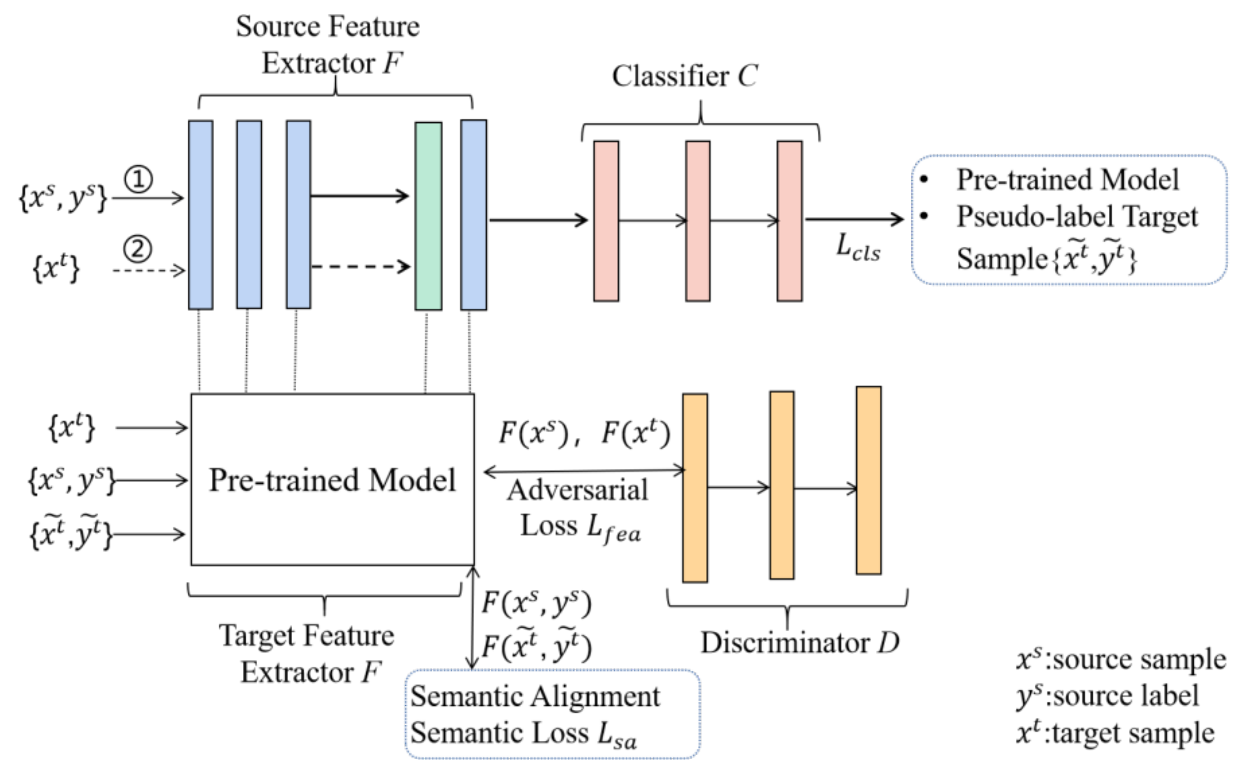
• A deep residual network with a self-attention module is used to extract features from multi-channels.
• We adopt the joint distribution alignment approach to reduce the distribution discrepancy. Firstly, inter-domain distribution discrepancy is reduced by adversarial learning. After that, class-level alignment can be achieved by optimizing the semantic alignment loss functions. Eventually, we can achieve intra-class sample compactness and inter-class sample separation.
• By the proposed model, massive experiments are done on two public malware datasets. Experimental findings show that the model can correctly classify unknown malware and has better accuracy than the existing detection models.

The remainder of this paper is organized as follows. Section 2 surveys the work related to malware detection and classification. A detailed description of our detection system is presented in Section 3. Section 4 demonstrates the experimental details and the related comparative results of our model and other known detection systems. Section 5 concludes this paper.

2. Related Work

The method of visualizing malware has the advantages of intuition and effectiveness, which has attracted extensive attention in the field of cyberspace security and industry. In this section, we discuss the detection methods of malware feature visualization, which are mainly divided into two categories: machine learning-based and transfer learning-based methods.

2.1. Machine Learning-Based Malware Detection

Machine learning (ML) algorithms have widespread applications, e.g., natural language processing, computer vision, automatic transmission, and cybersecurity. ML algorithms mainly are divided into two classifications: supervised and unsupervised learning. The former requires massive labeled data to train the model. Nataraj et al. [13] demonstrated that analyzing texture features of images could detect malware more accurately than existing malware analysis techniques. As a result, this method is widely used for malware detection. Generally, during detection malware, it converts malware raw files into gray-scale images and uses restored gray-scale images to train neural network models. Nataraj et al. [13] extracted GIST (Generalized Search Trees) features of gray-scale images and classified malware by K-Nearest Neighbor (KNN). Instead of extracting specific features, Hamad et al. [14] proposed a novel fine-grained Malware Image Classification Framework (MICS), which extracted hybrid features of malware and classified malicious family samples with the help of an SVM (Support Vector Machines) classifier. Firstly, they converted malicious programs into gray-scale images; then, they captured local and global features of images aiming at classifying malicious software. Jinpei et al. [15] presented the MalNet, a novel Deep Neural Network (DNN)-based malware detection framework, in which CNN (Convolutional Neural Networks) and LSTM (Long Short-Term Memory) networks were adopted to automatically extract features in order to reduce the expense of feature engineering. All these supervised learning methods rely on labeled data to train the model.

For unknown samples, the detection capability of the model will decrease. Different from supervised learning in malware classification, unsupervised learning by cluster quality optimization is based on sample similarity [16]. Pitolli et al. [17] proposed an online clustering algorithm named BIRCH (Balanced Iterative Reducing and Clustering using Hierarchies) to identify malware families. The algorithm could efficiently update the clusters with new samples emerging, and the algorithm could classify malware as an existing family and could also identify malware of unknown families. All these unsupervised detection methods must depend on a large amount of data to reach high accuracy. Additionally, some unsupervised algorithms extend the dataset based on the original malware file to detect new malware. Zahra et al. [18] generated unknown malware samples by deep generative adversarial networks. Together with the original samples, these generated samples were used to practice a more robust classifier for checking new malware variants.

The afore-mentioned ML methods have obtained a good performance. However, most approaches depend on expert knowledge to extract features. Meanwhile, with new malware increasing rapidly, extracting features faces the challenge of updating the features, which requires much time. This paper converts the raw files into gray-scale images and uses deep neural networks to extract features automatically and quickly. Moreover, to extract features more effectively, this paper introduces a self-attention module.

2.2. Transfer Learning-Based Malware Detection

Transfer learning (TL) can extract useful knowledge from one or more tasks in the source domain and apply the knowledge to new target tasks. Its essence is the transfer and reuse of knowledge. Currently, TL methods have been extensively applied to many fields [19,20,21,22,23]: for example, image classification [24], semantic segmentation [25], robot recognition [26], and medical areas [20]. Vasan et al. [9] improved the accuracy of malware detection and classification with the help of fine-tuning the parameters of the neural network, and they used data augmentation to address the data imbalance problem.

In addition to fine tuning, domain adaptation is another subfield of TL algorithms. Compared with fine tuning, the advantage of domain adaptation is that it makes full use of the feature similarity in the source and target domains. Therefore, the knowledge gained from the source domain can be transferred to the target domain. Bartos et al. [27] constructed domain-invariant feature representations of network traffic generated by malware. Nonetheless, they focused on designing a transformation that reduced the discrepancy of cross-domain feature distribution without considering the conditional distribution problem. Additionally, to detect unknown malware variants, Li et al. [28] proposed a framework named DART by taking advantage of adaptation regularization transfer learning. They detected malware variants by aligning the feature distributions of different domains. This method can lessen the difference of marginal distribution in the source and target domain. However, it does not take into account the difference in class distribution. Rong et al. [29] proposed TransNet to check unknown malware. Firstly, they converted malware traffic data into RGB images and then replaced the batch normalization layer with a transfer batch normalization layer to solve the domain shift problem. Finally, they used the RGB images as inputs of a DNN to solve the problem of data distribution discrepancy among multi-domains. However, they did not consider the class-level alignment of different domains. To get a better accuracy for malware detection, this paper proposes a novel approach based on unsupervised domain adaptation. It is helpful to reduce domain distribution differences and achieve class-level distribution alignment.

3. Method Description

3.1. Overview

To achieve a better accuracy in malware detection, we propose a distributed joint alignment unsupervised domain adaptation method to detect unknown malware, which solves the difficulty of obtaining labels, and obtain the distribution discrepancy between tested samples and training samples. The whole architecture is shown in Figure 1. In Figure 1, the unlabeled samples are extracted features and then classified, where the target feature extractor F and classifier C are trained by Figure 2. In Figure 2, the architecture mainly contains three components: feature extractor $F_{\phi }$ for extracting domain-invariant features, classifier $C_{\varphi }$ for malware classification, and domain discriminators $D_{\omega }$ for domain adversarial learning, where $\phi$, $\varphi$, and $\omega$ are learnable parameters. Firstly, we train the model using the source domain data to obtain a pre-trained model; then, we assign labels for the target domain samples using the trained model to obtain pseudo-labeled samples. Secondly, the source domain samples, target domain samples, and pseudo-labeled samples are input into the pre-trained model to achieve distribution alignment by adversarial training and semantic alignment. Finally, the trained feature extractor $F_{\phi }$ and classifier $C_{\varphi }$ are used to classify the target domain samples. Moreover, the self-attention module is introduced for more effectively extracting local and long-term features.

The labeled malware samples are treated as the source domain. In response to this, unlabeled malware is taken as the target domain. A transferable domain classifier is practiced to forecast the labels of target domain samples by the distributed joint alignment of different samples from the source and target domain. In this paper, let $D_s={\left\{\left(x_i^s,y_i^s\right)\right\}}_{i=1}^{n_s} , D_t=\{{\left(x_j^t\right)}_{j=1}^{n_t}$ be the source domain with labels and the target domain without labels, respectively, where $n_s$ denotes the number of malware in the source domain, $y_i^s$ denotes the label of the sample $x_i^s$, and $D_s$ and $D_t$ have a different distribution.

We classify malware by the following processing. Firstly, we train the feature extractor $F_{\phi }$ and binary classifier $C_{\varphi }$ using the source domain $D_s$ by supervised learning; thus, the pre-trained model is established. Then, the classifier assigns a label to a sample in the target domain by the pre-trained model. These samples in the target domain have obtained pseudo-labels, which are denoted as $\widetilde{D_t}$. Secondly, global alignment of the feature extractor and domain discriminator is achieved by adversarial learning in the source domain $D_s$ and target domain $D_t$. Finally, to make these intra-class samples more compact and inter-class samples more separate, we propose class-center semantic alignment. That is, the class centers of pseudo-labeled samples $\widetilde{D_t}$ are aligned to the class centers of labeled samples $D_s$ in the source domain. Therefore, our model needs to jointly optimize supervised classification loss $L_{cls}$, global domain adversarial loss $L_{fea}$, and class-level semantic alignment loss function $L_{sa}$. Hence, the overall optimization objectives are

$$L=L_{cls}+\alpha L_{fea}+\beta L_{sa}$$

(1)

where the hyperparameters $\alpha$ and $\beta$ are the influence factors of global alignment and semantic alignment, respectively.

In the remaining subsections, we will detail the self-attention module, global domain alignment, semantic alignment, and model training.

3.2. Self-Attention Module

For extracting features of the images better, we insert a self-attention module in the feature extractor [30]. This module enables each pixel to associate with others. Therefore, our module can settle the long-distance dependence problem among common convolutional structures, and this module achieves a better balance between improving the perceptual field and reducing the number of parameters. Consequently, as a complement to convolutional neural network, we integrate a self-attention mechanism for getting long-term, multi-level dependencies across the image region.

We place the self-attentive mechanism at the fourth block of the residual network due to two reasons. Firstly, the self-attention module can effectively extract local features and reduce the resolution of convolution. Moreover, it can aggregate the global information of the features. Therefore, the ability of the model to extract information has improved.

Figure 3 illustrates the workflow of the self-attention module. In the self-attention module, the feature map x is firstly obtained by convolution from the front few layers of the residual network. Furthermore, three feature maps $q\left(x\right)$, $k\left(x\right)$, and $v\left(x\right)$ are obtained by three $1\times 1$ convolution, respectively. During the process of obtaining feature maps, the dimensions of $q\left(x\right)$ and $k\left(x\right)$ remain identical; only the channel value changes, while $v\left(x\right)$ keeps the same dimensions and output channels unchanged. Then, we transpose $q\left(x\right)$ and multiply it by $k\left(x\right)$. The attention map ${\rho }_{j,i}$ of [H × W, H × W] is obtained by normalizing each row by the Softmax layer. Multiplying the attention map ${\rho }_{j,i}$ by $v\left(x\right)$, we can obtain a feature map [H × W, C]. Then, processing it by a $1\times 1$ convolution, the output h$\left(x\right)$ is reconstructed as [H × W × C]; then, we can obtain the feature map $O$.

To make the model learn the local information faster in the initial stage and then gradually use the self-attention mechanism as the network training, this paper introduces the parameter $\theta$. The parameter will be learned in the self-attention layer. We initialize the parameter to 0, indicating that the self-attention module has not worked at the beginning. The network will gradually learn more long-range features by the self-attention module as the training proceeds. Therefore, the final output $f$ is given by:

$$\left\{\begin{array}{c}{o}_j=h\left({{\displaystyle \sum }}_{i=1}^{N}softmax\left(q{\left(x_i\right)}^{⊺},k\left(x_j\right)\right)v\left(x_i\right)\right),\\ f_i=\theta o_i+x_i,\end{array}\right.$$

(2)

where $O=\left(o_1,o_2,\dots o_j,\dots o_N\right)$. In our model, we use the self-attention mechanism in the feature extractor. The output features $f$ of the attention layer are used as the input of the next residual block. Eventually, each pixel is associated with other pixels. In this way, we solve the long-distance dependence problem that exists in ordinary convolutional structures.

3.3. Global Domain Alignment

Considering the distribution discrepancy between emerging unknown malware (target domain) and known labeled malware (source domain), we propose an approach of global domain alignment to reduce the disparity of cross-domain feature distribution. The two types of approaches to obtain global domain alignment in computer vision are mainly non-adversarial domain alignment and adversarial domain alignment. Non-adversarial domain alignment minimizes the global distribution discrepancy of domains by different metrics, e.g., Maximum Mean Discrepancy (MMD) [31], KL [32], CORAL [33], Wasserstein Distance [34], etc. In contrast, adversarial domain adaptation methods are inspired by Generative Adversarial Networks (GAN) to learn domain invariant features [35].

This study utilizes adversarial domain alignment to align the feature distributions of two domains by minimizing the global domain adversarial loss function $L_{fea}$. That is, the feature extractor $F_{\phi }$ and the domain discriminator $D_{\omega }$ interrelate during the training process. To make the distribution of $D_t$ closer to the distribution of $D_s$, we initialize the target feature extractor $F_{\phi }$ using the pre-trained source model. Then, the feature extractor $F_{\phi }$ is corrected by adversarial training. In this mapping, we modify the target model to match the source distribution. This is most similar to the original generative adversarial learning. The $D_{\omega }$ is trained to minimize the domain loss $L_{fea}$ to distinguish the features between both domains, and the feature extractor $F_{\phi }$ obfuscates the domain discriminator $D_{\omega }$ by maximizing the domain loss $L_{fea}$ to acquire a domain-variant feature representation. When the training ends, the network can obtain domain-variant feature representation. The global domain alignment adversarial training loss can be expressed as follows:

$$L_{fea}\left(F_{\phi },D_{\omega }\right)=-{\mathbb{E}}_{x~D_t}\log \left[1-D_{\omega }\left(F_{\phi }\left(x_s\right)\right)\right]-{\mathbb{E}}_{x~D_s}\left[D_{\omega }\left(F_{\phi }\left(x_t\right)\right)\right].$$

(3)

3.4. Semantic Alignment

Currently, most of the existing domain adaptation-based malware classification methods focus only on global distribution alignment. However, global alignment alone does not achieve precise alignment. As shown in Figure 4, after global alignment, the source and target domains achieved global alignment, but there are still some misclassified samples. To make similar samples more compact, Weston et al. [36] calculated the distance among samples in the manifold embedding space and minimized this distance, but this requires a high computational cost. To reduce the computational cost, Wen et al. [37] calculated the absolute distance between each sample and its commensurable class center.

In this paper, to make the model have higher classification ability, we consider that not only the similar samples should be compact, but also the centers of different classes should be separate as much as possible. Based on this idea, we propose class center semantic alignment. The class center semantic alignment loss function $L_{sa}$ can be computed as follows:

$$L_{sa}={\displaystyle \sum }_{i=1}^{n}max\left(\frac{1}{2}\Vert x_i-c_{y_i}\Vert {}_2^2-r_1, 0\right)+\gamma {\displaystyle \sum }_{i,j=1}^{m}max\left(0,r_2-\Vert c_i-c_j\Vert {}_2^2\right),$$

(4)

where γ is a trade-off parameter, and n and m denote the volume of malware in a batch and a class, respectively. $c_{y_i}$ ($y_i\in \left\{1,2,\cdots ,m\right\}$) is the class center of the source domain and target domain alternately. $r_1$,$r_2$ are thresholds. $\Vert x_i-c_{y_i}\Vert {}_2^2$ is the distance from every sample to its class center. $\Vert c_i-c_j\Vert {}_2^2$ is the distance among the centers of the different classes. During the class center updating, it is based on a mini-batch rather than all samples in each epoch. Therefore, in each iteration, the class center is updated according to the following equation:

$$\Delta c_j=\left\{\begin{array}{cc}\frac{{{\displaystyle \sum }}_{i=1}^n{c}_j-x_i}{1+n},& y_i=j\\ 0,& y_i\ne j\end{array}\right.$$

(5)

$$c_j^{t+1}=c_j^t-\epsilon \Delta c_j^t,$$

(6)

where $n$ denotes the volume of samples in each batch, and $\epsilon$ represents a learning rate. In class center semantic alignment, we need to know the pseudo-label of a sample in the target domain to obtain center alignment. We define $\left\{p_c\left(x_i^t\right){|}_{c=1}^n\right\}$ as the probability in which $x_i^t$ belongs to the c-th class. We get the pseudo labels by the following steps. Firstly, the model is trained with the labeled data in the source domain. Secondly, we predict the labels of the target domain by the use of the trained model. The pseudo label corresponding to sample $x_i^t$ is calculated by ${\tilde{y}}_i^t=argma{x}_c{p}_c\left(x_i^t\right)$. The class label of $x_i^t$ is determined by the label with the maximum probability.

After performing semantic alignment, each sample belonging to the identical class is aligned to its class center, respectively. In this way, we can make similar data more compact and dissimilar data more discriminable in the feature space. Finally, all samples with identical labels will be aligned to the neighborhood of the shared class centers.

3.5. Model Training

In this paper, to get high detection and classification accuracy, we need to align their distribution of source and target domain. We achieve this goal through two steps: global alignment and semantic alignment. Firstly, global domain alignment is implemented with the help of adversarial learning. Then, semantic alignment is performed through minimizing the class center semantic alignment loss function $L_{sa}$ using Equation (4). Therefore, we need to jointly optimize supervised classification loss $L_{cls}$ (Cross Entropy Loss), global domain adversarial loss $L_{fea}$ using Equation (3), and semantic alignment loss $L_{sa}$. So, the whole loss function is represented in Equation (7),

$$L_{total}\left(X^S,Y^S,X^T,\widetilde{X^T}\right)=L_{cls}\left(X^S,Y^S;\phi ,\varphi \right)+\alpha L_{fea}\left(X^S,X^T;\phi ,\omega \right)+\beta L_{sa}\left(X^S,\widetilde{X^T}\right).$$

(7)

The specific training process is as follows. Firstly, we minimize the classification loss $L_{cls}$ by standard supervised learning with $D_s$. Thus, we get a pre-trained feature extractor $F_{\phi }$ and classifier $C_{\varphi }$. Secondly, during the process of computing all samples in a certain target domain, their pseudo-label is assigned by our pre-trained model according to ${\tilde{y}}_i^t=argma{x}_c{p}_c\left(x_i^t\right)$. Then, we initialize the feature extractor $F_{\phi }$ and classifier $C_{\varphi }$ of the target model by the use of the pre-trained model. Global alignment of the $D_s$ and the $D_t$ is achieved through minimizing the global domain adversarial loss $L_{fea}$. Meanwhile, class center semantic alignment is implemented by minimizing loss function $L_{sa}$. Algorithm 1 gives out the whole training process of the proposed method.

Algorithm 1 Training of our model

Input: Source domain: $D_s={\left\{\left(x_i^s,y_i^s\right)\right\}}_{i=1}^{n_s}$, Target domain: $D_t={\left\{x_j^t\right\}}_{j=1}^{n_t}$, Pseudo-label: ${\tilde{y}}_i^t=argma{x}_c{p}_c\left(x_i^t\right)$. Output$: F_{\phi }$,$C_{\varphi }$,$D_{\omega }$. Initialize: $\mathrm{a} \mathrm{parameter} \mathrm{set} \mathrm{of} \mathrm{target} \mathrm{model} \mathsf{\Omega }=\left\{\phi ,\varphi ,\omega ,\alpha ,\beta ,\epsilon \right\}$ 1: While do 2:          Sample mini batch ds, dt and construct a batch in DS, Dt do 3:          for t = 1 to batchsize do 4:               Use ds to compute source domain class Center cs and ct←cs. 5:               Compute Δcj by Equation (6) and update class $c_j^{t+1}=c_j^t-\epsilon \Delta c_j^t$ 6:               Compute semantic alignment loss $L_{sa}$ by Equation (4). 7:               Compute joint loss function $L_{total}\left(X^S,Y^S,X^T,\widetilde{X^T};\phi ,\varphi ,\omega \right)$ 8:               Back propagate $L_{total}$ to get the gradient value of each parameter 9:               The parameter $\mathrm{set} \mathsf{\Omega }$ is updated by gradient descent with Adam optimizer 10:          end for 11:          Calculate mean loss and mean accuracy 12: end while

4. Experiment and Result Analysis

4.1. Experimental Settings

4.1.1. Dataset

Our approach is evaluated on two public window malware datasets (BIG-2015 and Malimg) and a benign dataset selected from the Playdrone [38], respectively. BIG-2015 is a publicly available malware dataset from Microsoft on the Kaggle platform. The BIG-2015 dataset contains 21,741 samples belonging to nine categories. Among them, 10,868 samples are used for training, and 10,873 are testing ones. This experiment only utilizes the training malware. We use the byte file to generate the malware gray-scale image and normalize it to a fixed size. The Malimg dataset includes 9,339 malware from 25 malware families.

Table 1. BIG-2015 dataset set.

No	Family	Class	Family
1	Virus	Ramnit	1541
2	Trojan	Vundo	475
3	Trojan	Lollipop	2478
4	Trojan	Gatak	1013
5	Botnet	Simda	42
6	Malware Attack	Traceur	751
7	Trojan	Kelihos_ver1	398
8	Trojan	Kelihos_ver3	2942
9	Trojan Downloader	Obfuscator.ACY	1228

and

Table 2. Malimg dataset set.

No.	Family	Samples	No.	Family	Samples
1	Yuner.A	800	14	Instantaccess	431
2	Wintrim.BX	97	15	Fakerean	381
3	VB.AT	408	16	Dontovo.A	162
4	Swizzor.gen!I	132	17	Dialplatform.B	177
5	Swizzor.gen!E	128	18	C2LOP.P	146
6	Skintrim.N	80	19	C2LOP.gen!g	200
7	Rbot!gen	158	20	Autorun.K	106
8	Obfuscator.AD	142	21	Alueron.gen!J	198
9	Malex.gen!J	136	22	Allaple.L	1591
10	Lolyda.AT	159	23	Allaple.A	2949
11	Lolyda.AA3	123	24	Agent.FYI	116
12	Lolyda.AA2	184	25	Adialer.C	122
13	Lolyda.AA1	213	26	Total	9339

demonstrate the details about the two datasets.

In addition to malware, in our experiment, we also use 2280 benign samples. We randomly select a family in the malware dataset as the target domain, whereas the remainder is treated as the source domain. In addition, 1140 benign samples are included in the source and target domain, respectively. For example, in the BIG-2015 dataset, the Ramnit family is used for the unlabeled target domain, and the remaining families are from the source domain. The benign samples are different in the two domains.

4.1.2. Implementation Details

In our experiment, all malware in BIG-2015 and benign software are converted into gray-scale images and normalized to the size of 196 × 196 pixels. The original sample of the Malimg dataset is the gray-scale image, so we only transform it into a fixed size of 196 × 196 pixels. On each dataset, one of the families is selected as the target domain, and the remaining families are used as source domains. In this way, for the BIG-2015 dataset, there are nine tasks; for the Malimg dataset, there are 25 tasks. This study uses a residual network as our feature extractor and classifier. We insert the self-attention module before the fourth residual block. The adversarial discriminator has the same structure with the classifier, which consists of three fully connected layers, and the size of each layer is x-2048-4096-1 (where x is the size of the input feature), respectively. A ReLU activation function is used in each layer, and we use the dropout mechanism to reduce overfitting by ignoring several neurons with a probability in each training batch. The entire training process uses the Adam optimizer, where the learning rate is 0.0001 and the weight decay is 0. The pre-training source domain uses a cross-entropy loss function $L_{cls}$. During the training process, we simultaneously optimize $L_{cls}$, the domain adversarial loss function $L_{fea}$, and the semantic alignment loss function $L_{sa}$. The parameters are $\alpha =0.1$ and $\beta =0.1$, respectively. Another learning rate $\epsilon$ at the local class center update is set to 0.5. Domain adversarial loss is scaled by 0.1. The two thresholds r1, r2 used in the semantic alignment loss function are 0 and 100, respectively. The batch size is 32. Experiments are performed in the PyTorch framework. The experimental equipment is a personal computer. Its configuration includes the following: CPU: IntelI CITM) i5-4590 3.30GHz 3.30 GH; RAM: 4GB; OS: Windows 7.

4.1.3. Evaluation Metrics

The study uses the following four metrics to evaluate the effect of every model: Accuracy, Precision, Recall, and F1-score. All samples can be classified according to the true and predicted label, and the following factors are introduced:

True Positive (TP) means that the true label is positive, and the predicted label is positive.

True Negative (TN) means that the true label is negative, and the predicted label is negative.

False Positive (FP) means that the true label is negative, while the predicted label is positive.

False Negative (FN) means that the true label is positive, while the predicted label is negative.

Accuracy denotes the ratio of correctly classified samples to the total number of samples.

$$Accuracy=\frac{TP+TN}{TP+TN+FP+FN}.$$

(8)

Precision is the ratio of positive samples to forecasted positive samples.

$$Precision=\frac{TP}{TP+FP}.$$

(9)

Recall refers to the ratio of predicted positive samples out of all actually positive samples.

$$Recall=\frac{TP}{TP+FN}.$$

(10)

F1-score denotes a weighted mean of Recall and Precision. As a comprehensive metric, it is introduced to balance the effects of accuracy and recall, and to evaluate a classifier more comprehensively.

$$F1\text{-}\mathit{score}=2\times \frac{precision\times recall}{precision+recall}.$$

(11)

4.2. Performance Comparison of Different Models

In this paper, we have run extensive experiments and calculated four evaluation metrics mentioned above when each family acts as an unknown malware (target domain) on the two datasets. We also take into consideration that one dataset (e.g., BIG-2015) is treated as the source data, and another (e.g., Malimg) is the target data. In the experiments, the benign software used in the source and target domain is distinct, too. Figure 5 and Figure 6 illustrate the experimental results. We can see that we achieve good results with our approach for each subtask. We averaged the results over several tests to obtain an average accuracy and recall of 95.04% and 94.25%, respectively on the BIG-2015 dataset, and the average accuracy and recall on the Malimg dataset are 95.63% and 95.30%, respectively.

In addition, we compare our work with some existing malware detection methods.

Table 3. Performance comparison of our method with previous domain adaptation-based work.

Method	Accuracy	Recall	Precision	F1-Score
BIRCH [17]	95.02%	90.2%	95.2%	92.3%
DART [28]	93.9%	91.2%	89.8%	90.0%
GAA-ADS [39]	92.8%	91.3%	-	-
RCNN+Transfer Learning [40]	92.8%	-	95.6%	-
Proposed method (Malimg)	95.63	95.30%	95.34%	94.98%
Proposed method (BIG-2015)	95.04%	94.25%	95.10%	94.65%

demonstrates our performance comparison.

We also make a comparison between our work with some existing domain adaptation-based methods such as BIRCH [17], DART [28], GAA-ADS [39], and RCNN+ transfer learning [40], which are shown in Table 3. Our method obtains a higher accuracy and recall than the GAA-ADS and RCNN + transfer learning. Our method is also higher than the DART, which uses the distribution alignments. DART mitigates the domain discrepancy by optimizing the marginal and manifold distributions of two domains. However, they do not take into account semantic alignment. In this paper, to facilitate feature extraction, we transform the raw PE files into gray-scale images before feeding them into the neural network, and a self-attention module is introduced for capturing long-distance dependency. Our model obtains a higher accuracy and recall by jointly aligning the global and semantic alignment. From the above data, the proposed method has a better performance compared with some approaches only considering global domain adaptation, and it also confirms that semantic information can improve the classification accuracy.

5. Conclusions

This paper studies the detection of Windows unknown malware. To solve the difficulty in obtaining labeled samples and the problem of the discrepancy in the distribution between unknown and source samples, we propose an efficient deep unsupervised domain adaptation for unknown malware detection. Firstly, we adopt the joint distribution alignment approach to reduce the distribution discrepancy. We minimize the discrepancy of the distribution between the source and target domains to learn shared feature representation by adversarial learning. To further obtain semantic information about the unlabeled samples, we minimize the distance from the labeled source domain and the pseudo-labeled target domain samples to the class center. Then, to enhance feature extraction ability, we adopt a residual network with a self-attention mechanism as the pre-trained model. Finally, extensive experiments are conducted on two datasets, and the results illustrate that the proposed method outperforms the state-of-art domain adaptation-based detection methods in detecting unknown malware. In future work, we will investigate a more advanced fine-grained domain adaptation approach for malware family classification and conduct extensive experiments on different datasets (e.g., Android malware, IoT malware).

References

1. Malware Statistics [EB/OL]. Available online: https://www.av-test.org/en/statistics/malware/ (accessed on 1 January 2022).
2. Jung, B.H.; Bae, S.I.; Choi, C.; Im, E.G. Packer identification method based on byte sequences. Concurr. Comput. Pract. Exp. 2020, 32, e5082. [Google Scholar] [CrossRef]
3. Yuan, Z.; Lu, Y.; Xue, Y. Droiddetector: Android malware characterization and detection using deep learning. Tsinghua Sci. Technol. 2016, 21, 114–123. [Google Scholar] [CrossRef]
4. Shijo, P.V.; Salim, A. Integrated static and dynamic analysis for malware detection. Procedia Comput. Sci. 2015, 46, 804–881. [Google Scholar] [CrossRef] [Green Version]
5. Imran, M.; Afzal, M.T.; Qadir, M.A. Using hidden markov model for dynamic malware analysis: First impressions. In Proceedings of the 12th International Conference on Fuzzy Systems and Knowledge Discovery (FSKD), Zhangjiajie, China, 15–17 August 2015; pp. 816–821. [Google Scholar]
6. Damodaran, A.; Di Troia, F.; Visaggio, C.A.; Austin, C.A.; Stamp, M. A comparison of static, dynamic, and hybrid analysis for malware detection. J. Comput. Virol. Hacking Tech. 2017, 13, 1–12. [Google Scholar] [CrossRef]
7. Vasan, D.; Alazab, M.; Wassan, S.; Naeem, H.; Safaei, B.; Zheng, Q. IMCFN: Image-based malware classification using fine-tuned convolutional neural network architecture. Comput. Netw. 2020, 171, 107–138. [Google Scholar] [CrossRef]
8. Rafique, M.F.; Ali, M.; Qureshi, A.S.; Khan, A.; Mirza, A.M. Malware Classification using Deep Learning based Feature Extraction and Wrapper based Feature Selection Technique. arXiv 2019, arXiv:1910.10958. [Google Scholar]
9. Vasan, D.; Alazab, M.; Wassan, S.; Naeem, H.; Safaei, B.; Zheng, Q. Image-based malware classification using ensemble of CNN architectures (IMCEC). Comput. Secur. 2020, 92, 101748. [Google Scholar] [CrossRef]
10. Catak, F.O.; Ahmed, J.; Sahinbas, K.; Khand, Z.H. Data augmentation-based malware detection using convolutional neural networks. PeerJ Comput. Sci. 2021, 7, e346. [Google Scholar] [CrossRef]
11. Arora, A.; Peddoju, S.K.; Chouhan, V.; Chaudhary, A. Hybrid Android malware detection by combining supervised and unsupervised learning. In Proceedings of the 24th Annual International Conference on Mobile Computing and Networking, New York, NY, USA, 15 October 2018; pp. 798–800. [Google Scholar]
12. Wilson, G.; Cook, D.J. A survey of unsupervised deep domain adaptation. ACM Trans. Intell. Syst. Technol. 2020, 11, 1–46. [Google Scholar] [CrossRef] [PubMed]
13. Nataraj, L.; Yegneswaran, V.; Porras, P. A comparative assessment of malware classification using binary texture analysis and dynamic analysis. In Proceedings of the ACM Conference on Computer and Communications Security, New York, NY, USA, 21 October 2011; pp. 21–30. [Google Scholar]
14. Naeem, H.; Guo, B.; Naeem, R.M. A light-weight malware static visual analysis for IoT infrastructure. In Proceedings of the 2018 International Conference on Artificial Intelligence and Big Data (ICAIBD), Chengdu China, 26–28 May 2018; pp. 240–244. [Google Scholar]
15. Yan, J.; Qi, Y.; Rao, Q. Detecting malware with an ensemble method based on deep neural network. Secur. Commun. Netw. 2018, 2018, 7247095. [Google Scholar] [CrossRef] [Green Version]
16. Alom, M.Z.; Taha, T.M. Network intrusion detection for cyber security using unsupervised deep learning approaches. In Proceedings of the 2017 IEEE National Aerospace and Electronics Conference (NAECON), Dayton, OH, USA, 27–30 June 2017; pp. 63–69. [Google Scholar]
17. Pitolli, G.; Laurenza, G.; Aniello, L.; Querzoni, L.; Baldoni, R. MalFamAware: Automatic family identification and malware classification through online clustering. Int. J. Inf. Secur. 2021, 20, 371–386. [Google Scholar] [CrossRef]
18. Moti, Z.; Hashemi, S.; Namavar, A. Discovering future malware variants by generating new malware samples using generative adversarial network. In Proceedings of the 9th International Conference on Computer and Knowledge Engineering (ICCKE), Mashhad, Iran, 24–25 October 2019; pp. 319–324. [Google Scholar]
19. Sun, Q.; Liu, Y.; Chua, T.S.; Schiele, B. Meta-transfer learning for few-shot learning. In Proceedings of the IEEE Conference on Computer Vision and Pattern Recognition (CVPR), Long Beach, CA, USA, 16–20 June 2019; pp. 403–412. [Google Scholar]
20. Pathak, Y.; Shukla, P.K.; Tiwari, A.; Stalin, S.; Singh, S. Deep transfer learning-based classification model for COVID-19 disease. IRBM, 2020; online ahead of print. [Google Scholar] [CrossRef]
21. Wang, J.; Chen, Y.; Feng, W.; Yu, H.; Huang, M.; Yang, Q. Transfer learning with dynamic distribution adaptation. ACM Trans. Intell. Syst. Technol. (TIST) 2020, 11, 1–25. [Google Scholar] [CrossRef] [Green Version]
22. Neyshabur, B.; Sedghi, H.; Zhang, C. What is being transferred in transfer learning? arXiv 2020, arXiv:2008.11687. [Google Scholar]
23. Celik, Y.; Talo, M.; Yildirim, O.; Karabatak, M.; Acharya, U.R. Automated invasive ductal carcinoma detection based using deep transfer learning with whole-slide images. Pattern Recognit. Lett. 2020, 33, 232–239. [Google Scholar] [CrossRef]
24. Rezende, E.; Ruppert, G.; Carvalho, T.; Theophilo, A.; Ramos, F.; Geus, P. Malicious software classification using VGG16 deep neural network’s bottleneck features. Adv. Intell. Syst. Comput. 2018, 738, 51–59. [Google Scholar]
25. Cui, B.; Chen, X.; Lu, Y. Semantic segmentation of remote sensing images using transfer learning and deep convolutional neural network with dense connection. IEEE Access 2020, 8, 116744–116755. [Google Scholar] [CrossRef]
26. Sorocky, M.J.; Zhou, S.; Schoellig, A.P. Experience selection using dynamics similarity for efficient multi-source transfer learning between robots. In Proceedings of the 2020 IEEE International Conference on Robotics and Automation (ICRA), Paris, France, 31 May–31 August 2020; pp. 2739–2745. [Google Scholar]
27. Bartos, K.; Sofka, M.; Franc, V. Optimized invariant representation of network traffic for detecting unseen malware variants. In Proceedings of the 25th USENIX Security Symposium, USENIX, Austin, TX, USA, 10–12 August 2016; pp. 807–822. [Google Scholar]
28. Li, H.; Chen, Z.; Spolaor, R. Dart: Detecting unseen malware variants using adaptation regularization transfer learning. In Proceedings of the ICC 2019—2019 IEEE International Conference on Communications (ICC), Shanghai, China, 1 May 2019; pp. 1–6. [Google Scholar]
29. Rong, C.; Gou, G.; Cui, M.; Xiong, G.; Li, Z.; Guo, L. TransNet: Unseen malware variants detection using deep transfer learning. Lect. Notes Inst. Comput. Sci. 2020, 336, 84–101. [Google Scholar]
30. Zhang, H.; Goodfellow, I.; Metaxas, D.; Odena, A. Self-attention generative adversarial networks. arXiv 2019, arXiv:1805.08318v2. [Google Scholar]
31. Zhu, Y.; Zhuang, F.; Wang, J.; Chen, J.; Shi, Z.; Wu, W.; He, Q. Multi-representation adaptation network for cross-domain image classification. Neural Netw. 2019, 119, 214–221. [Google Scholar] [CrossRef]
32. Zhuang, F.; Cheng, X.; Luo, P.; Pan, S.J.; He, Q. Supervised representation learning: Transfer learning with deep autoencoders. In Proceedings of the Twenty-Fourth International Joint Conference on Artificial Intelligence, Palo Alto, CA, USA, 27 June 2015; pp. 4119–4125. [Google Scholar]
33. Sun, B.; Feng, J.; Saenko, K. Return of frustratingly easy domain adaptation. In Proceedings of the Thirtieth Conference on Artificial Intelligence, Phoenix, AZ, USA, 2 March 2016; pp. 2058–2065. [Google Scholar]
34. Courty, N.; Flamary, R.; Tuia, D.; Rakotomamonjy, A. Optimal transport for domain adaptation. IEEE Trans. Pattern Anal. Mach. Intell. 2017, 39, 1853–1865. [Google Scholar] [CrossRef] [PubMed]
35. Tzeng, E.; Hoffman, J.; Saenko, K.; Darrell, T. Adversarial discriminative domain adaptation. In Proceedings of the Conference on Computer Vision and Pattern Recognition, Honolulu, HI, USA, 21–26 July 2017; pp. 2962–2971. [Google Scholar]
36. Weston, J.; Ratle, F.; Mobahi, H.; Collobert, R. Deep learning via semi-supervised embedding. In Neural Networks: Tricks of the Trade 2012; Montavon, G., Orr, G.B., Eds.; Springer Press: Berlin/Heidelberg, Germany, 2012; Volume 7700, pp. 639–655. [Google Scholar]
37. Wen, Y.; Zhang, K.; Li, Z.; Qiao, Y. A discriminative feature learning approach for deep face recognition. In Computer Vision—ECCV 2016; Leibe, B., Matas, J., Eds.; Springer: Cham, Switzerland, 2016; Volume 9911, pp. 499–515. [Google Scholar]
38. Ficco, M. Detecting IoT malware by Markov chain behavioral models. In Proceedings of the 2019 IEEE International Conference on Cloud Engineering (IC2E), Prague, Czech Republic, 24–27 June 2019; pp. 229–234. [Google Scholar]
39. Moustafa, N.; Slay, J.; Creech, G. Novel geometric area analysis technique for anomaly detection using trapezoidal area estimation on large-scale networks. IEEE Trans. Big Data 2017, 5, 481–494. [Google Scholar] [CrossRef]
40. Zhao, Y.; Cui, W.; Geng, S.; Bo, B.; Feng, Y.; Zhang, W. A malware detection method of code texture visualization based on an improved faster RCNN combining transfer learning. IEEE Access 2020, 8, 166630–166641. [Google Scholar] [CrossRef]
Figure 1. The whole architecture of our model.
Symmetry 14 00296 g001
Figure 2. The training process of the target feature extractor F and classifier C.
Symmetry 14 00296 g002
Figure 3. The workflow of the self-attention module.
Symmetry 14 00296 g003
Figure 4. Sample distribution alignment process. The yellow circle and green circle denote the source and target domain, respectively. The triangle represents benign samples, and the circle represents malicious samples.
Symmetry 14 00296 g004
Figure 5. Detection performance of unknown malware on the BIG-2015 dataset.
Symmetry 14 00296 g005
Figure 6. Detection performance of unknown malware on the Malimg dataset.
Symmetry 14 00296 g006