Detecting Compressed Deepfake Images Using Two-Branch Convolutional Networks with Similarity and Classifier

Abstract

As a popular technique for swapping faces with someone else’s in images or videos through deep neural networks, deepfake causes a serious threat to the security of multimedia content today. However, because counterfeit images are usually compressed when propagating over the Internet, and because the compression factor used is unknown, most of the existing deepfake detection models have poor robustness for the detection of compressed images with unknown compression factors. To solve this problem, we notice that an image has a high similarity with its compressed image based on symmetry, and this similarity is not easily affected by the compression factor, so this similarity feature can be used as an important clue for compressed deepfake detection. A TCNSC (Two-branch Convolutional Networks with Similarity and Classifier) method that combines compression factor independence is proposed in this paper. The TCNSC method learns two feature representations from the deepfake image, i.e., similarity of the image and its compressed counterpart and authenticity of the deepfake image. A joint training strategy is then utilized for feature extraction, in which the similarity characteristics are obtained by similarity learning while obtaining authenticity characteristics, so the proposed TCNSC model is trained for robust feature learning. Experimental results on the FaceForensics++ (FF++) dataset show that the proposed method significantly outperforms all competing methods under three compression settings of high-quality (HQ), medium-quality (MQ), and low-quality (LQ). For the LQ, MQ, and HQ settings, TCNSC achieves 91.8%, 93.4%, and 95.3% in accuracy, and outperforms the state-of-art method (Xception-RAW) by 16.9%, 10.1%, and 4.1%, respectively.

1. Introduction

Deepfake is a counterfeiting technique that aims to replace a targeted person’s face in a video with someone else’s face. This term was first introduced when a Reddit user known as “deepfakes” claimed in 2017 that he had built a machine learning system that enabled him to swap celebrity faces into pornographic movies. In recent years, credit to the emergence and development of Generative Adversarial Networks (GAN) [1] and Variational Auto-Encoder (VAE) [2], anyone may now create a genuinely appearing face whose identity does not exist in the real world or execute facial alterations in a video with a high level of realism. Furthermore, there are more and more face-changing softwares available for direct downloads, such as Zao, REFACE, FaceApp, Audacity, Soundforge, etc., and a user can quickly generate fake images or videos by supplying a few pictures. Therefore, if this kind of technology is allowed to develop freely, it will bring many security challenges to society, economy, politics, and other aspects.

Fortunately, large efforts are being made by many research teams to design new algorithms for face manipulation detection. Most deepfake detection algorithms identify the authenticity by detecting whether there are suspicious forged traces in the images or videos, and most of them have made significant improvements by taking advantage of a convolutional neural network (CNN) in extracting the texture features in image spatial domain, such as FWA [3], Face X-ray [4], MPSM [5], PELF [6], Multi-attention [7], etc., or by using the benifit of Recurrent Neural Network (RNN) in extracting the temporal features, such as EyeBlinking [8], HeadPose [9], etc. Traces of forgery in uncompressed images are more obvious in FaceForensics++ datasets [10]; as shown in Figure 1a, unlike the real image, the face in the fake image is significantly warped. The difference between real and fake images makes the forensics of uncompressed images relatively easy.

Nowadays, compressed images are widely used in actual social networks due to storage capacity and network bandwidth limitations. Most methods do not consider the scenario when the deepfake images are compressed, e.g., JPEG and WEBP, especially with relatively large compression factors. XceptionNet [10] achieved 99.7% accuracy in raw images, but the accuracy decreased to 81.3% in low-quality compressed images. When the fake images are compressed, compressed blocking artifacts appear in the compressed fake images. As shown in Figure 1b–d, both the compressed real image and compressed fake image produce compression artifacts, which makes it difficult to distinguish them. Moreover, the image quality after compression also has a greater impact on deepfake detection. The lower the image quality, the more obvious the compressed blocking artifacts, as shown in Figure 1c,d. We can also train multiple models to cope with the effects of different compression factors, but this is invalid for an unknown compression factor. Therefore, the forensics of compressed deepfake images has become a very important issue, especially in scenarios where the compression factor is unknown. To settle this problem, according to our observations that images and their compressed images have many similarities based on symmetry, a novel compressed deepfake detection neural network is presented in this paper for robust forgery face detection against various compression factors.

Specifically, TCNSC is a two-branch network that combines a similarity-learning branch and a binary-classification branch, which uses the symmetrical raw images and their compressed images as input, and is optimized by simultaneously training these two branches. The core idea of this method is that the features that determine the authenticity of an image is not affected by image compression. Essentially, we use the method of contrastive learning to realize the similarity learning between a symmetrical original image and its compressed image, and then we can extract the general features of this image. Since this symmetry will always exist, we only need to compress the original image without considering the specific compression factor in this process. Experimental results on the FaceForensics++ dataset demonstrate the superior performance of the proposed method over other state-of-the-art methods for the detection of facial tampered contents under various compression factors. The main contributions in this paper are as follows:

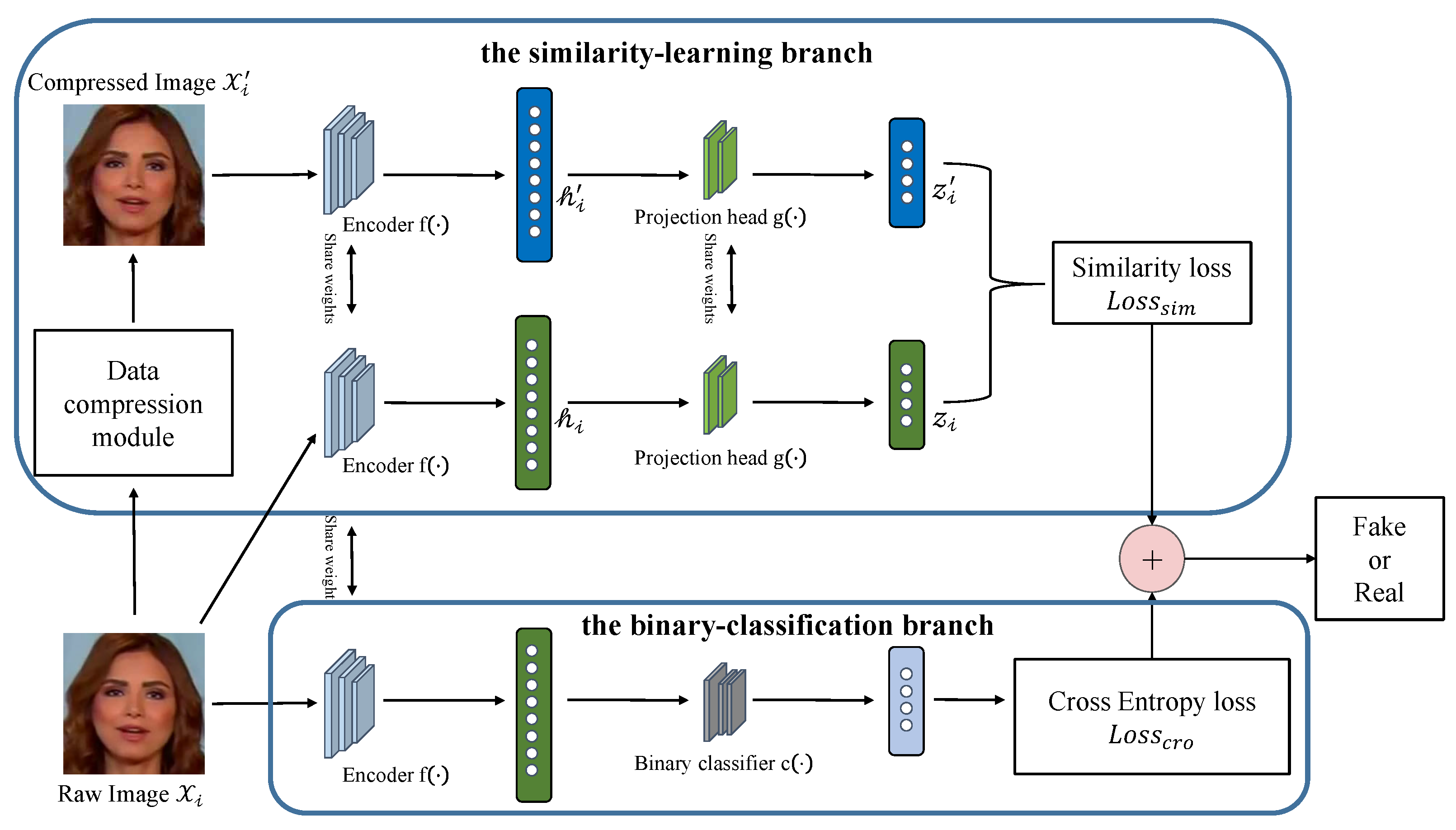
• A two-branch convolutional network for robust compressed deepfake detection is proposed based on symmetry of an image and its compressed image.
• The proposed method can determine the authenticity of a raw image or its various compressed images. In other words, our method is robust to the compression factor.
• A joint loss function is introduced to train the similarity-learning branch and binary-classification branch simultaneously, which can extract the common features under image compression and identify the authenticity of the image.
• Various experiments are conducted to test our method and compare it with state-of-the-art deepfake detection methods.

The rest of this paper is organized as follows: Section 2 reviews the related research work of deepfake detection and contrastive learning. Section 3 introduces the method proposed in this paper. We explain and analyze the experimental results in Section 4. Section 5 concludes this paper.

2. Related Works

In this section, we will firstly review previous deepfake detection methods and then look back upon recent works on similarity learning.

2.1. Deepfake Detection Methods

In recent years, deepfake detection is a research hotspot. Existing deepfake detection methods mainly focus on detecting traces left during deepfake generation, such as temporal and spatial artifact traces. FWA [3] used convolutional neural networks to capture the artifacts created during face region fusion to determine the authenticity of the image. DSP-FWA [11] is a further improved method based on FWA, it includes a spatial pyramid pooling (SPP) module [12] to better deal with the changes in the resolution of the original face. Rossler et al. [10] directly trained an XceptionNet [13] as a binary classifier on the FaceForensics++ dataset, and in order to improve the detection accuracy under various compression factors, the Xception network trains three models respectively for the RAW, C23, and C40 (C23 and C40 are compressed videos in the FF++ dataset) videos. The Xception-RAW and Xception-C23 are effective when the compression factor is small, but the detection accuracy decreases when the compression factor is large. Furthermore, the Xception-C40 model gets the best performance when the compression factor is larger, but the detection accuracy also drops when the compression factor is small. Nguyen et al. [14] used VGG19 [15] to extract latent features and input features into a capsule network to realize the detection of forged images and videos. Afchar et al. [16] proposed the MesoNet network, which can focus on the microscopic characteristics of videos and images, and train a binary classifier in a supervised manner. Face X-ray [4] observes that the processed facial image is always fused with the existing background image; therefore, the difference on the boundary can be used as a signal to detect the manipulated fake face. Chen et al. [5] propose a Multi-scale Patch Similarity Module (MPSM) for mining the difference between real area and forged area, so as to realize the detection of face forgery. Gu et al. [6] propose a progressive enhancement learning framework to exploit both the RGB and fine-grained frequency clues, and to decouple true and false traces in the frequency domain space. Through this progressive feature enhancement process, this method can effectively use fine-grained frequency information and RGB information to locate subtle traces of forgery. Zhao et al. [7] describe deepfake detection as a fine-grained classification problem and propose a new multi-attention deepfake detection network, and propose to use the attention mechanism to make the network pay attention to different local information. The texture feature enhancement block can amplify the sub-texture defects in the shallow features, so as to achieve the identification of authenticity. Sun et al. [17] propose a Dual Contrastive Learning (DCL), which constructs positive and negative paired data and carries out contrastive learning at different granularities to learn generalized feature representation. Frank et al. [18] find that critical artifacts are introduced due to the upsampling techniques in GANs and investigate the artifacts revealed in the frequency domain. Jung et al. [19] proposed a method to detect deepfakes by identifying an anomaly based on the time, repetition, and intervened eye-blinking duration within videos. Gu et al. [20] propose a novel sampling unit named snippet, which contains a few successive video frames for local temporal inconsistency learning, and this method uses the local motion information to include the motion inconsistency between frames to identify the authenticity of the video.

However, none of the above methods consider the scenario of image compression. When an image is compressed, compression block artifacts appear in the compressed image. This compressed block artifact can greatly confuse these detectors and miscalculate them. Unlike the above method, the TCNSC method in this paper uses similarity between an image and its compressed image, which is not easy with the compression factor. Experiments show that this detection method—based on the two-branch network—can achieve high detection accuracy and strong robustness on the FaceForensics++ dataset. The specific experimental analysis is provided in Section 4.2. Robustness here means that a detection method can have high detection accuracy in three different situations, namely, detection of image forgery with high compression quality (HQ), detection of image forgery with medium compression quality (MQ), and detection of image forgery with low compression quality (LQ).

2.2. Similarity Learning

In order to realize the similarity learning between the original image and the compressed image, this paper adopts a contrastive learning method. The contrastive learning method is a self-supervised learning approach that uses the similarity or difference of the model learning dataset without labels to determine the general properties of the dataset. Major advances in contrastive learning, such as Deep InfoMax, MoCo, and SimCLR, have put a spotlight on the representational potential of discriminative models. Deep InfoMax [21] is the first to use a contrastive learning task to explicitly model mutual information, maximizing the mutual information between a local patch and its global context. In MoCo [22], researchers expand on the idea of using momentum contrast to leverage instance discrimination, which significantly raises the number of negative samples. The authors of SimCLR [23] add to the importance of a hard positive sample strategy by introducing data augmentation. SimCLR uses an end-to-end training framework rather than MoCo’s momentum contrast. SimCLR learns representations by using a contrastive loss in the latent space to maximize agreement between different augmented views of the same data example. Since the SimCLR can better obtain the similarity features of the original image and its compressed image, this method is adopted in the similarity learning in this paper; we modified the loss function and narrowed the number of samples per batch during the training phase. The specifics are presented in Section 3.1.

3. Analysis and Method

In this section, the specific contents of the method proposed in this paper are introduced, including the overall framework of the similarity learning convolutional network and the joint loss function.

Figure 2 shows our proposed method of compressed deepfake image detection. The method includes two branches: the similarity-learning branch and binary-classification branch. The similarity-learning branch is a CNN trained to obtain similarity characteristics. The compressed image is similar to its raw uncompressed image regardless of the compression factor, in other words, the similarity characteristics are also not disturbed by the compression factor. First, we construct the input paired dataset by a data compression module. Then, the paired datasets are input to an encoder, f(·), which can extract the image representation separately. Again, image representation from the encoder f(·) is input to a projection head, g(·), which individually maps the image representation to the space where similarity loss is applied. Finally, we apply cosine distance to measure similarity of the image representation, and the similarity loss function is constructed and optimized. The binary-classification branch is a CNN trained to determine the authenticity of the image. First, the train dataset is sent to the encoder, f(·), which shares parameters with the encoder in the similarity-learning branch, and the representation vectors can be achieved. Next, the representation vectors are fed into the binary classifier c(·) to perform a true and false binary classification task by optimizing the cross-entropy loss function. Moreover, we jointly optimize the similarity loss function and the cross-entropy loss function, so that we can try to preserve the features used for true and false identification in the process of similarity learning. See Architecture Section 3.1 for details.

3.1. Architecture

Our method is robustly put forward to compressed deepfake detection by obtaining features for discriminating image authenticity unaffected by image lossy compression.

The similarity-learning branch is a convolutional neural network (CNN) that extracts common features from the raw images and their compressed images. It consists of three parts: a data compression module, an encoder f(·), and a projection head g(·). Algorithm 1 summarizes the similarity-learning branch.

Algorithm 1: Main algorithm in the similarity-learning branch

Step 1: We assume that a dataset of images with sampled Batch Size N is D=$\left\{X_i,y_i\right\}$, where $X_i$ represents the i-th image and its label is denoted as $y_i$.

Steps 2–4: For the given input image $X_i$, it will be compressed by the data compression module, and then we can construct a new paired symmetric dataset, denoted $\left\{X_i,X_i^{\prime },y_i\right\}$, where $X_i^{\prime }$ is the compressed image of $X_i$.

Steps 5–9: This new paired symmetric dataset $\left\{X_i,X_i^{\prime },y_i\right\}$ will be individually fed into the encoder in the similarity-learning branch for similarity learning.

Step A: The encoder f(·) is a convolutional neural network that extracts representation vectors h from the paired symmetric dataset $\left\{X_i,X_i^{\prime },y_i\right\}$. We use the classic ResNet18 [24] network as the encoder to obtain the pair of representation vectors ($h_i$ = f($X_i$), $h_i^{\prime }$ = f($X_i^{\prime }$)), where $h_i$ is the raw image representation vectors and $h_i^{\prime }$ is its corresponding compressed image representation vector.

Step B: To improve the effect of similarity learning, a projection head g(·) maps the paired symmetric representation vectors ($h_i$, $h_i^{\prime }$) to the same space where similarity loss is applied. The projection head g(·) consists of two linear layers and a ReLU [25] nonlinear layer, and then we obtain a symmetric pair of feature vectors ($z_i$ = g($h_i$), $z_i^{\prime }$ = g($h_i^{\prime }$)), where $z_i$ is the representation vectors of the raw image after mapping and $z_i^{\prime }$ is its corresponding compressed image representation vectors after mapping.

Step C: After the above process, we can construct the similarity loss function and use cosine distance to measure how similar an image is to its compressed image, which is shown in Equation (1):

$$cos(z_i,z_i^{\prime })=\frac{z_i\ast z_i^{\prime }}{\parallel z_i{\parallel }_2\ast {\parallel z_i^{\prime }\parallel }_2}$$

(1)

where $z_i$ is the feature vector of the raw image, $z_i^{\prime }$ is the feature vector of its compressed image.

Step 10: Suppose we have N samples and with the data compressed augmentation, the batch size will become 2N. Therefore, a similarity loss function can be applied to a batch of samples, which is shown in Equation (2):

$$Los{s}_{sim}(X_i,X_i^{\prime })=\frac{1}{2N}(\sum _{n=1}^N(1-cos(z_i,z_i^{\prime }))+\sum _{n=1}^N(1-cos(z_i^{\prime },z_i)))$$

(2)

The binary-classification branch is applied to the common features from the similarity-learning branch and outputs binary labels for evaluation purposes. It is made up of the encoder f(·) and a binary classifier c(·). The encoder shared parameters with the encoder in the similarity-learning branch discussed earlier and its output is the representation vectors ($h_i$, $h_i^{\prime }$). Algorithm 2 summarizes the binary-classification branch.

Algorithm 2: Main algorithm in the binary-classification branch

Step 1: We assume that a dataset of images with sampled Batch Size N is D = $\left\{X_i,y_i\right\}$.

Steps 2–5: Sampled batch size N from train set D.

Step A: Sampled images are fed into encoder f(·), and the representation vectors of these images are obtained.

Step B: The representation vectors are fed into the binary classifier c(·) for true or false identification training.

Step 6: Thus, the cross-entropy loss is applied to train the binary classification, which is shown in Equation (3):

$$Los{s}_{cro}=\frac{1}{N}(\sum (-[y_i\ast log(p_i)+(1-y_i)\ast log(1-p_i)]))$$

(3)

where $y_i$ represents the label of an image and $p_i$ is the probability that this image is predicted to be true.

3.2. Loss Function

The final loss function is formulated by integrating the facial authenticity classification and the similarity loss, which is shown in Equation (4):

$$Los{s}_{total}=Los{s}_{cro}+\lambda \ast Los{s}_{sim}$$

(4)

where $\lambda$ is the balanced parameter for the compression feature.

4. Experiment and Evaluation

4.1. Experimental Setting

Dataset. FaceForensics++ (FF++) [13] is a benchmark dataset and is widely used for deepfake detection evaluation. The FF++ dataset contains 1000 real videos, and all real videos undergo four counterfeiting methods, including DeepFakes (DF) [26], Face2Face (F2F) [27], FaceSwap (FS) [28], and NeuralTexures (NT) [29]. In our work, we use the 1000 real videos and 1000 fake videos faked by the DF method. We randomly employ 700 real videos and the corresponding fake videos for training, 150 real videos and corresponding fake videos for validation, and 150 real videos and corresponding fake videos for testing.

Train Set. Following the settings in [10], 300 frames are sampled from each of 700 pairs of training videos and 150 pairs of validation videos to form an image-based dataset, and then we adopted MTCNN [30] for face detection and cropping. The cropped image is resized to 224 ∗ 224 ∗ 3 as the network inputs. Depending on the compression quality factor in the data compression module in Section 3.1, we constructed four different train sets for the two branch network proposed in this paper, (RAW,HQ), (RAW,MQ), (RAW,LQ), and (LQ,MQ), where RAW is the uncompressed raw image, HQ is a high-quality compressed image with a compression quality factor of 20, MQ is a medium-quality compressed image with a compression quality factor of 50, and LQ is a low-quality compressed image with a compression quality factor of 80.

Test Set. Simiilar to the method of extracting faces from the train set, we also sampled 300 frames from each of 150 pairs of testing videos to form a basic test set. To evaluate the robustness of compressed image detection, we performed compression processing on the images in the basic test set under three different compression quality factors, including high-quality (HQ, compression quality factors set to 80), medium-quality (MQ, compression quality factors set to 50), and low-quality (LQ, compression quality factors set to 20). To evaluate the performance of different compression algorithms, we also used the WEBP [31] algorithm to compress these images in the basic test set. Therefore, we constructed 5 test sets, including RAW, HQ, MQ, LQ, and WEBP; when testing, we verified these 5 test sets separately.

Implementation Details. In our implementation, the PyTorch framework was used and trained on the NVIDIA GEFORCE RTX 2080 Ti GPU platform. We used the ADAM optimizer with a learning rate of 0.0001, where the exponential learning rate scheduler was adopted. The network was trained for 10k iterations with the batch size set as 64. In this paper, the evaluation metric accuracy was used to evaluate the proposed method. It can be computed by:

$$accuracy=\frac{N_{correct}}{N_{total}}$$

(5)

where $N_{correct}$ represents the number of correctly classified images, and $N_{total}$ is the total number of images.

4.2. Evaluation

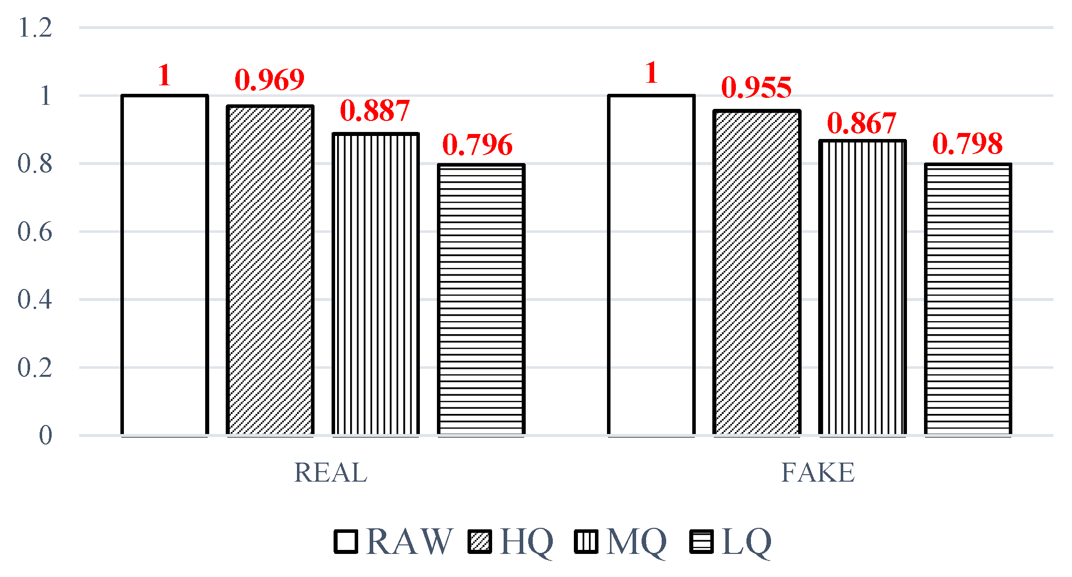
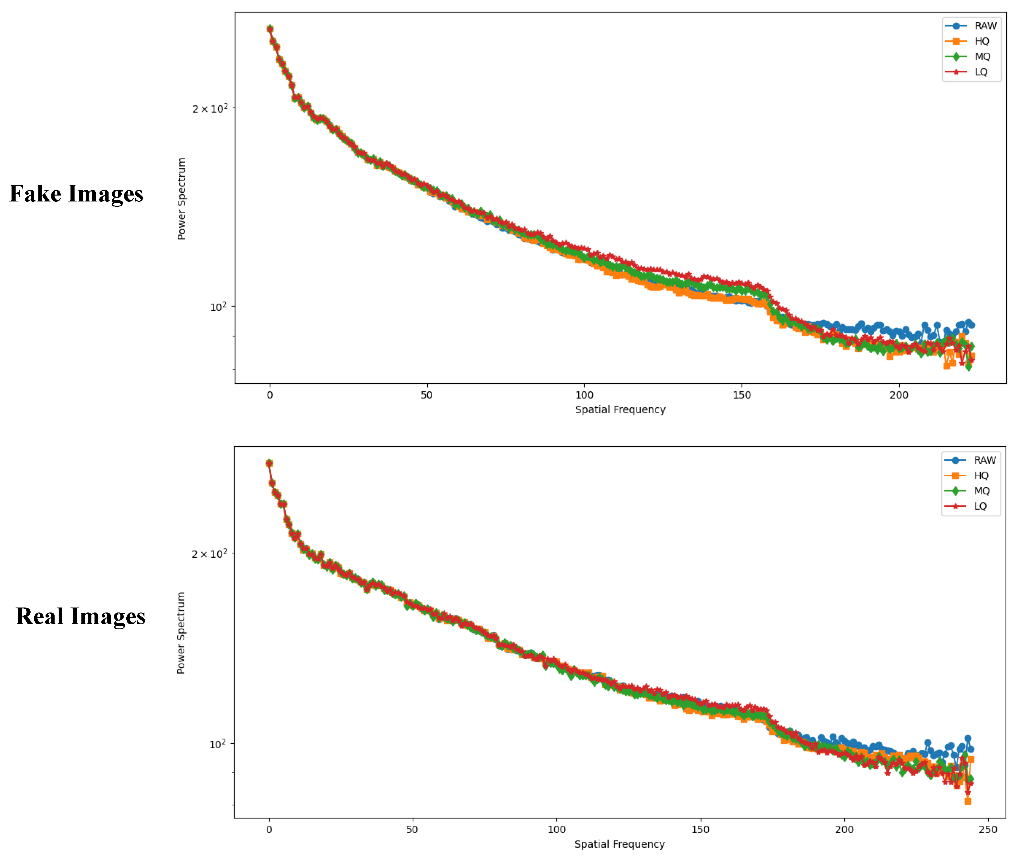
4.2.1. Impact of Compression Factor

As previously analyzed, the core of the TCNSC method lies in the success of extracting general characteristics of deepfake images that are not affected by image lossy compression. It is important to evaluate the effect of the compression factors on performance. To analyze the impact of the compression factors, we implement the cross-image lossy compression experiments and show the results in

Table 1. The comparisons of the cross-image lossy compression detection accuracy (%). (RAW, LQ) indicates that the training dataset consists of the raw images and their LQ compressed images. The bold results are the best.

Training Dataset	Test Dataset
	RAW	HQ	MQ	LQ	WEBP
(RAW, HQ)	96.8	94.5	92.6	90.4	89.2
(RAW, MQ)	96.4	94.3	92.1	90.2	89.3
(RAW, LQ)	97.6	95.3	93.4	91.8	92.7
(LQ, MQ)	93.2	92.1	91.4	91.1	89.1

. We trained several models with different symmetric training datasets constructed from the raw images and their compressed images with three compression factors, and then we used these trained models to verify the authenticity of the multiple compressed images. From the test results, the detection accuracy of each model for images with a certain compression factor was roughly the same, and training with (RAW, LQ) was the best model, which performed slightly better than other models. Therefore, the detection result may not have much relationship with the compression factor of the image lossy compression, because similarity learning can obtain general characteristics of the image that are not affected by image lossy compression. In other words, the general features of an image can be obtained by itself, regardless of the specific compression factor, and the authenticity of this image can be identified.

4.2.2. Ablation Study

To show the effect of each branch separately, we compare the single branch with our proposed dual-branch method. First, we detect the images by using the similarity-learning branch individually, denoted as model A. The results of the single similarity-learning branch are shown in the first row of

Table 2. Comparison of detection accuracy (%) between single-branch and dual-branch ablation experiments. The bold results are the best.

Model	Test Dataset
	RAW	HQ	MQ	LQ	WEBP
model A	51.8	51.7	51.7	51.7	51.7
model B	98.8	96.2	83.7	71.3	82.6
dual-branch model	97.6	95.3	93.4	91.8	92.7

, and the detection accuracy is lower than our proposed dual-branch method. Second, we only implement the binary-classification branch to detect images, denoted as model B. As shown in the second row of Table 2, although the detection results are good when the compressiong factor is small, the detection accuracy rate has been decreasing as the compression factor increases. In the third row of Table 2, we can see that combining the two branches obtains the best result, especially in the case of a high compression factor. The fusion of two branches could reveal both tampering artifacts and similarity features, contributing to better performance than a single branch network. Therefore, the merging of the two branches can improve the performance of compressed deepfake image detection.

4.2.3. Comparisons with Other Deepfake Detection Methods

In this subsection, the detection accuracy of our proposed method is compared with other deepfake detection methods, including Xception [10], MesoNet [16], Capsule network [14], and DSP-FWA [11]. First, when the test dataset is in raw images, the detection accuracies of the different methods are shown in the second column in

Table 3. Detection accuracies (%) of different methods against compressed images with various compression factors. The bold results are the best.

Methods	RAW	HQ	MQ	LQ	WEBP
Xception-RAW Xception-C23 Xception-C40 [10]	99.7 99.3 81.3	91.2 90.6 86.0	83.3 86.7 87.9	74.9 82.1 88.3	82.6 85.2 86.5
MesoInception Meso4 [16]	91.7 89.1	57.4 51.3	57.4 50.8	57.2 50.4	57.2 51.4
Capsule [14]	94.47	89.2	81.3	64.8	78.5
FWA [3]	81.6	76.8	67.2	58.1	68.4
DSP-FWA [11]	93.4	87.6	83.1	75.6	82.8
Ours	97.6	95.3	93.4	91.8	92.7

. It can be observed that most methods perform well with accuracies higher than 90% in free of image compression, and the accuracy of our method reached 97.6%, which is slightly lower than the Xception method and higher than other methods. Then, when the test dataset is compressed with three compression factors, the detection accuracies of the different methods are shown in the remaining columns in Table 3. Due to the introduction of similarity learning, we obtain the general characteristics of the image that are not affected by image lossy compression, so even if the image is compressed, our method can still effectively detect the authenticity, and experimental results confirm it. As shown in Table 3, the detection accuracy of our method only decreased by about 5.94% with LQ setting, while the Xception-RAW method decreased by about 24.87%, the Xception-C23 method decreased by about 17.32%, and the other remaining methods decreased by more than 20%. To illustrate the reasons for the performance degradation, we randomly selected 1000 real images and 1000 fake images from the test dataset as the input of the Xception network and our method, and visualized them using the T-SNE [32] algorithm. In Figure 3, we see that raw real and fake images are separated with a margin, but as the compression factor increases, this margin becomes smaller and smaller, and even large area overlaps have appeared, which is also one of the reasons for the performance degradation.

To more intuitively understand why the TCNSC method works, we visualize the feature map in Figure 4. Following the method used in [33], we generated Gradient-weighted Class Activation Mapping (Grad-CAM) of our method. Grad-CAM helps us successfully distinguish between important nodes and non-important nodes in the image. Thus, we can observe the activation of the original weighted neuron on the image to display the image with a high probability. It can be seen that although the test images are compressed, the main areas of concern of TCNSC are basically symmetrical. The results show that the method has strong robustness under different compression factors.

4.3. Discussion

As every one knows, the purpose of image lossy compression is to represent images with less data to save storage costs or transmission time. After using lossy compression algorithms, the original image cannot be restored completely. Lossy compression is usually based on techniques by removing details that the human eye typically does not notice. In other words, lossy compression does not affect the human eye’s perception of image content, so images before and after compression have similar characteristics. We use SSIM (Structural Similarity Metric) [34] to measure the similarity of images before and after compression. Figure 5 shows the SSIMs between compressed images and the original image. The higher the SSIM value (scale 0.0–1.0), the higher the similarity of the images, and a value of 1 represents exactly the same. We can observe that when HQ, the SSIM values of the real image, and the fake image are close to 1, indicating that the difference between the HQ image and the original image is small. Compared with the raw image, when MQ, the SSIM of the real image and the fake image decrease by 11.3% and 13.3%, respectively, and when LQ, the SSIM of the real image and the fake image drop by 20.4% and 20.2% respectively. Although compressed images have varying degrees of distortion, there are still similarities between them.

Furthermore, in the frequency domain of an image, the Azimuthal Average is applied to compute a 1D representation of the Fast Fourier Transform power spectrum [35]. Figure 6 displays the power spectrum of the raw images and several compressed images. The power spectrum in the low-frequency region is roughly unchanged, while the high-frequency region has a few fluctuations. Therefore, the lossy compression of the image has a relatively large impact on the high-frequency information, and has a small impact on the middle and low frequencies. Based on the above analysis, the general features extracted by similarity-learning are very likely to be distributed in the mid-low frequency region.

However, there is another key factor that hinders the successful application of similarity learning. Experiments in the paper [36] show that deepfake detection exploits the difference between high-frequency regions in real images and fake images. Generally, the low-frequency region is related to the content of an image, while the high-frequency region is related to the edges and texture information of an image. Compared to true maps, false maps show more energy in high-frequency regions. Compared to the real image, the fake image shows more energy in the high frequency region. For this reason, we believe that it is usually not easy to design a convolutional neural network based solely on similarity learning to extract ground-truth features from compressed images. Hence, similarity learning, although very effective in learning the general features of an image by teaching the model which data points are similar or different, without human participation, it has limited usage in handling the compressed deepfake detection task at hand. The results of the ablation experiment in Section 4.2.2 show that applying the similarity-learning branch alone to detect deepfake is not efficient. That is why in this work, we adopt an approach with a dual-branch convolutional neural network to perform the compressed deepfake detection by training the similarity-learning and binary-classification simultaneously.

5. Conclusions and Future work

In this paper, a novel similarity-learning convolutional network is proposed for compressed deepfake images detection under various compression factors. The proposed method uses the raw images and their arbitrary compression factor images as a training set for training the common characteristics without being affected by image compression, and can also identify the authenticity of the image. Specifically, a joint learning strategy, including similarity-learning and binary-classification learning, is developed for robust authentic feature learning. Common features of images are extracted using the similarity-learning branch and can be used to judge the authenticity of images. Extensive experiments indicate that the proposed framework achieves superior performance over other reference methods on the FaceForensics++ dataset, especially for challenging low and unknown compression quality scenes. Certainly, the authenticity of compressed fake videos is also very important. Therefore, a robust method with temporal information is the goal of our future work.

References

1. Goodfellow, I.; Pouget-Abadie, J.; Mirza, M.; Xu, B.; Warde-Farley, D.; Ozair, S.; Courville, A.; Bengio, Y. Generative adversarial nets. Adv. Neural Inf. Process. Syst. 2014, 27, 2672–2680. [Google Scholar]
2. Kingma, D.P.; Welling, M. Auto-encoding variational bayes. arXiv 2013, arXiv:1312.6114. [Google Scholar]
3. Li, Y.; Lyu, S. Exposing deepfake videos by detecting face warping artifacts. arXiv 2018, arXiv:1811.00656. [Google Scholar]
4. Li, L.; Bao, J.; Zhang, T.; Yang, H.; Chen, D.; Wen, F.; Guo, B. Face X-ray for more general face forgery detection. In Proceedings of the IEEE/CVF Conference on Computer Vision and Pattern Recognition, Seattle, WA, USA, 13–19 June 2020; pp. 5001–5010. [Google Scholar]
5. Chen, S.; Yao, T.; Chen, Y.; Ding, S.; Li, J.; Ji, R. Local relation learning for face forgery detection. In Proceedings of the AAAI Conference on Artificial Intelligence, Virtual, 2–9 February 2021; Volume 35, pp. 1081–1088. [Google Scholar]
6. Gu, Q.; Chen, S.; Yao, T.; Chen, Y.; Ding, S.; Yi, R. Exploiting fine-grained face forgery clues via progressive enhancement learning. In Proceedings of the AAAI Conference on Artificial Intelligence, Virtually, 22 February–1 March 2022; Volume 36, pp. 735–743. [Google Scholar]
7. Zhao, H.; Zhou, W.; Chen, D.; Wei, T.; Zhang, W.; Yu, N. Multi-attentional deepfake detection. In Proceedings of the IEEE/CVF Conference on Computer Vision and Pattern Recognition, Nashville, TN, USA, 20–25 June 2021; pp. 2185–2194. [Google Scholar]
8. LIY, C.M.; InIctuOculi, L. ExposingAICreated FakeVideosbyDetectingEyeBlinking. In Proceedings of the 2018 IEEE International Workshop on Information Forensics and Security (WIFS), Hong Kong, China, 11–13 December 2018. [Google Scholar]
9. Yang, X.; Li, Y.; Lyu, S. Exposing deep fakes using inconsistent head poses. In Proceedings of the ICASSP 2019-2019 IEEE International Conference on Acoustics, Speech and Signal Processing (ICASSP), Brighton, UK, 12–17 May 2019; pp. 8261–8265. [Google Scholar]
10. Rossler, A.; Cozzolino, D.; Verdoliva, L.; Riess, C.; Thies, J.; Nießner, M. Faceforensics++: Learning to detect manipulated facial images. In Proceedings of the IEEE/CVF International Conference on Computer Vision, Seoul, Republic of Korea, 27–28 October 2019; pp. 1–11. [Google Scholar]
11. Li, Y.; Lyu, S. Exposing DeepFake Videos By Detecting Face Warping Artifacts. In Proceedings of the IEEE Conference on Computer Vision and Pattern Recognition Workshops (CVPRW), Long Beach, CA, USA, 16–17 June 2019. [Google Scholar]
12. He, K.; Zhang, X.; Ren, S.; Sun, J. Spatial pyramid pooling in deep convolutional networks for visual recognition. IEEE Trans. Pattern Anal. Mach. Intell. 2015, 37, 1904–1916. [Google Scholar] [CrossRef] [PubMed] [Green Version]
13. Chollet, F. Xception: Deep learning with depthwise separable convolutions. In Proceedings of the IEEE Conference on Computer Vision and Pattern Recognition, Honolulu, HI, USA, 21–26 July 2017; pp. 1251–1258. [Google Scholar]
14. Nguyen, H.H.; Yamagishi, J.; Echizen, I. Capsule-forensics: Using capsule networks to detect forged images and videos. In Proceedings of the ICASSP 2019-2019 IEEE International Conference on Acoustics, Speech and Signal Processing (ICASSP), Brighton, UK, 12–17 May 2019; pp. 2307–2311. [Google Scholar]
15. Simonyan, K.; Zisserman, A. Very deep convolutional networks for large-scale image recognition. arXiv 2014, arXiv:1409.1556. [Google Scholar]
16. Afchar, D.; Nozick, V.; Yamagishi, J.; Echizen, I. Mesonet: A compact facial video forgery detection network. In Proceedings of the 2018 IEEE International Workshop on Information Forensics and Security (WIFS), Hong Kong, China, 11–13 December 2018; pp. 1–7. [Google Scholar]
17. Sun, K.; Yao, T.; Chen, S.; Ding, S.; Li, J.; Ji, R. Dual contrastive learning for general face forgery detection. In Proceedings of the AAAI Conference on Artificial Intelligence, Virtually, 22 February–1 March 2022; Volume 36, pp. 2316–2324. [Google Scholar]
18. Frank, J.; Eisenhofer, T.; Schönherr, L.; Fischer, A.; Kolossa, D.; Holz, T. Leveraging frequency analysis for deep fake image recognition. In Proceedings of the International Conference on Machine Learning, Virtually, 13–18 July 2020; pp. 3247–3258. [Google Scholar]
19. Jung, T.; Kim, S.; Kim, K. Deepvision: Deepfakes detection using human eye blinking pattern. IEEE Access 2020, 8, 83144–83154. [Google Scholar] [CrossRef]
20. Gu, Z.; Chen, Y.; Yao, T.; Ding, S.; Li, J.; Ma, L. Delving into the local: Dynamic inconsistency learning for deepfake video detection. In Proceedings of the AAAI Conference on Artificial Intelligence, Virtually, 22 February–1 March 2022. [Google Scholar]
21. Hjelm, R.D.; Fedorov, A.; Lavoie-Marchildon, S.; Grewal, K.; Bachman, P.; Trischler, A.; Bengio, Y. Learning deep representations by mutual information estimation and maximization. arXiv 2018, arXiv:1808.06670. [Google Scholar]
22. He, K.; Fan, H.; Wu, Y.; Xie, S.; Girshick, R. Momentum contrast for unsupervised visual representation learning. In Proceedings of the IEEE/CVF Conference on Computer Vision and Pattern Recognition, Seattle, WA, USA, 13–19 June 2020; pp. 9729–9738. [Google Scholar]
23. Chen, T.; Kornblith, S.; Norouzi, M.; Hinton, G. A simple framework for contrastive learning of visual representations. In Proceedings of the International Conference on Machine Learning, Virtually, 13–18 July 2020; pp. 1597–1607. [Google Scholar]
24. He, K.; Zhang, X.; Ren, S.; Sun, J. Deep residual learning for image recognition. In Proceedings of the IEEE Conference on Computer Vision and Pattern Recognition, Las Vegas, NV, USA, 27–30 June 2016; pp. 770–778. [Google Scholar]
25. Agarap, A.F. Deep learning using rectified linear units (relu). arXiv 2018, arXiv:1803.08375. [Google Scholar]
26. Deepfakes. Available online: https://github.com/deepfakes/faceswap (accessed on 24 February 2022).
27. Thies, J.; Zollhofer, M.; Stamminger, M.; Theobalt, C.; Nießner, M. Face2face: Real-time face capture and reenactment of rgb videos. In Proceedings of the IEEE Conference on Computer Vision and Pattern Recognition, Las Vegas, NV, USA, 27–30 June 2016; pp. 2387–2395. [Google Scholar]
28. FaceSwap. Available online: https://github.com/MarekKowalski/FaceSwap (accessed on 24 February 2022).
29. Thies, J.; Zollhöfer, M.; Nießner, M. Deferred neural rendering: Image synthesis using neural textures. ACM Trans. Graph. (TOG) 2019, 38, 1–12. [Google Scholar] [CrossRef]
30. Yin, X.; Liu, X. Multi-task convolutional neural network for pose-invariant face recognition. IEEE Trans. Image Process. 2017, 27, 964–975. [Google Scholar] [CrossRef] [PubMed] [Green Version]
31. Ginesu, G.; Pintus, M.; Giusto, D.D. Objective assessment of the WebP image coding algorithm. Signal Process. Image Commun. 2012, 27, 867–874. [Google Scholar] [CrossRef]
32. Van der Maaten, L.; Hinton, G. Visualizing data using t-SNE. J. Mach. Learn. Res. 2008, 9, 2579–2605. [Google Scholar]
33. Selvaraju, R.R.; Cogswell, M.; Das, A.; Vedantam, R.; Parikh, D.; Batra, D. Grad-cam: Visual explanations from deep networks via gradient-based localization. In Proceedings of the IEEE International Conference on Computer Vision, Venice, Italy, 22–29 October 2017; pp. 618–626. [Google Scholar]
34. Wang, Z.; Simoncelli, E.P.; Bovik, A.C. Multiscale structural similarity for image quality assessment. In Proceedings of the Thrity-Seventh Asilomar Conference on Signals, Systems & Computers, Pacific Grove, CA, USA, 9–12 November 2003; Volume 2, pp. 1398–1402. [Google Scholar]
35. Durall, R.; Keuper, M.; Pfreundt, F.J.; Keuper, J. Unmasking deepfakes with simple features. arXiv 2019, arXiv:1911.00686. [Google Scholar]
36. Durall, R.; Keuper, M.; Keuper, J. Watch your up-convolution: Cnn based generative deep neural networks are failing to reproduce spectral distributions. In Proceedings of the IEEE/CVF Conference on Computer Vision and Pattern Recognition, Seattle, WA, USA, 14–19 June 2020; pp. 7890–7899. [Google Scholar]
Figure 1. Examples of several compressed real and fake images. The top row shows fake images, while the lower row shows real images. (a) The original (RAW) fake and real images are shown, with very obvious forged traces on the fake image. (b) The high-quality (HQ) fake and real images are shown, with more obvious forged traces on fake images, and the compressed blocking artifacts are not distinct. (c) The medium-quality (MQ) fake and real images are shown, with more obvious compressed blocking artifacts, and blurring of forged traces. (d) The low-quality (LQ) fake and real images are shown, with very obvious compressed blocking artifacts, and blurring of forged traces.
Symmetry 14 02691 g001
Figure 2. Overall network framework of our proposed method, and the whole framework consists of the similarity-learning branch and binary-classification branch. The similarity-learning branch consists of a data compression module, an encoder f(·), and a projection head g(·). The binary-classification branch is made up of the encoder f(·) and a binary classifier c(·). In the training phase, paired raw images and their compressed images are separately fed into the bottom and top networks of the similarity-learning branch, and the raw images are also fed into the binary-classification branch. The binary-classification branch for various compression images is used in the test phase.
Symmetry 14 02691 g002
Figure 3. The visualization of features using T-SNE. The first row shows the T-SNE visualization of the features obtained by our proposed method (TCNSC). The second row shows the T-SNE visualization of the features obtained by the Xception network [10]. (a) T-SNE visualization of RAW images. (b) T-SNE visualization of medium-quality (MQ) images. (c) T-SNE visualization of low-quality (LQ) images.
Symmetry 14 02691 g003
Figure 4. The heatmap visualization of the TCNSC method. The first row shows the Grad-CAM of the fake image, and the second row shows the Grad-CAM of the real image. (a) Grad-CAM heatmap of RAW images. (b) Grad-CAM heatmap of high-quality (HQ) images. (c) Grad-CAM heatmap of medium-quality (MQ) images. (d) Grad-CAM heatmap of low-quality (LQ) images.
Symmetry 14 02691 g004
Figure 5. SSIMs between the original image and the compressed images. Distortion is measured by calculating the similarity of images before and after compression. These images consist of 100 real images and 100 fake images, which are randomly selected from FF++ dataset [10].
Symmetry 14 02691 g005
Figure 6. The 1D Power Spectrum of the raw images and several compressed images. The top row is the spectrogram of the fake images and the bottom row is the spectrogram of the real images. In the lower right corner of each spectrogram, the high-frequency difference of each spectrogram is large, while the middle-frequency and low-frequency difference are small. The test images consist of 100 real images and 100 fake images, which are randomly selected from FF++ dataset [10].
Symmetry 14 02691 g006