Some New Time and Cost Efficient Quadrature Formulas to Compute Integrals Using Derivatives with Error Analysis

Abstract

In this research, some new and efficient quadrature rules are proposed involving the combination of function and its first derivative evaluations at equally spaced data points with the main focus on their computational efficiency in terms of cost and time usage. The methods are theoretically derived, and theorems on the order of accuracy, degree of precision and error terms are proved. The proposed methods are semi-open-type rules with derivatives. The order of accuracy and degree of precision of the proposed methods are higher than the classical rules for which a systematic and symmetrical ascendancy has been proved. Various numerical tests are performed to compare the performance of the proposed methods with the existing methods in terms of accuracy, precision, leading local and global truncation errors, numerical convergence rates and computational cost with average CPU usage. In addition to the classical semi-open rules, the proposed methods have also been compared with some Gauss–Legendre methods for performance evaluation on various integrals involving some oscillatory, periodic and integrals with derivative singularities. The analysis of the results proves that the devised techniques are more efficient than the classical semi-open Newton–Cotes rules from theoretical and numerical perspectives because of promisingly reduced functional cost and lesser execution times. The proposed methods compete well with the spectral Gauss–Legendre rules, and in some cases outperform. Symmetric error distributions have been observed in regular cases of integrands, whereas asymmetrical behavior is evidenced in oscillatory and highly nonlinear cases.

1. Introduction

Numerical analysis has a rich store of methods to find the answer by purely arithmetical operations. Many practical problems in applied sciences and mathematical physics are given in the form of integrals. Different analytical techniques are available to compute such integrals; several numerical techniques have been developed to obtain approximate solutions for various classes of integrals. The methods of numerical integration are sometimes referred to as quadrature rules because these are used to approximate the integrals of the functions of one variable. As quadrature rules provide a very close estimate of the actual integration in most critical problems, the numerical evaluation of integrals through these techniques has been a key topic in mathematical research. These formulas are used for calculating the area under the region defined by the integrand within a range, finite or infinite, and when the integrand either cannot be integrated analytically or values are given in a tabular form only without its explicit mathematical description then numerical integration is the only option [1,2]. The worst cases consist of a definite integral whose analytical evaluation is not possible especially when these are associated with singularities and nonlinearities in solving differential and integral equations [2,3], for example:

$${{\displaystyle \int }}_0^1\frac{e^{-x}}{x^{\frac{2}{3}}}dx,{{\displaystyle \int }}_0^1\frac{e^{x^{-2}}}{\sqrt{1-x^2}}dx,{{\displaystyle \int }}_{-\infty }^1\sin x^{2}dx, \mathrm{and} {{\displaystyle \int }}_0^1\frac{\sin x}{x}dx$$

(1)

The efficiency of quadrature rules is usually categorized in terms of the degree of precision and order of accuracy. Therefore, obtaining higher precision and accuracy in numerical integration formulas becomes one of the challenges in the field of numerical analysis. A numerical integration formula is generally given as:

$${{\displaystyle \int }}_a^{b}f\left(x\right)dx\approx {\displaystyle \sum }_{i=0}^n{c}_{i}f\left(x_i\right)$$

(2)

where the constant $c_i$ are the weights and $x_0, x_1, \dots , x_n$ are $n+1$ equidistant nodes in the interval $\left[a, b\right]$. The Formula (2) represents Newton–Cotes quadrature rules, in general, form. In the semi-open Newton–Cotes formulae, the function evaluation at one of the endpoints of the interval is excluded. In this paper, we excluded the endpoint, which is on the right side of the interval, i.e., nodes at equally spaced points of $\left[a,b\right)$ are considered. We can rewrite (2) as:

$${{\displaystyle \int }}_a^{b}f\left(x\right)dx\approx {{\displaystyle \int }}_{x_0}^{x_n}f\left(x\right)dx\approx {\displaystyle \sum }_{i=0}^{n-1}{c}_{i}f\left(x_i\right)$$

(3)

where $x_0, x_1, \dots , x_{n-1}$ are distinct 𝑛 integration points and $c_i$ are 𝑛 weights within the interval $\left[a, b\right)$ with $x_i=a ih$, $i=0, 1, 2, \dots , n-1$, and $h=\left(b-a\right)/ \left(n+1\right)$.

The starting semi-open Newton–Cotes quadrature rule in basic form along with the local error term is defined as:

$${{\displaystyle \mathbf{\int }}}_{\mathit{a}}^{\mathit{b}}\mathit{f}\left(\mathit{x}\right)\mathit{d}\mathit{x}=\left(\mathit{b}-\mathit{a}\right)\mathit{f}\left(\mathit{a}\right)+\frac{{\left(\mathit{b}-\mathit{a}\right)}^{\mathbf{2}}}{\mathbf{2}}{\mathit{f}}^{\prime }\left(\mathit{\xi }\right)$$

(4)

where $\xi \in \left(a,b\right)$ and is known as the one-point semi-open Newton–Cotes rule. The composite form of this method with the global error term is defined as:

$${{\displaystyle \int }}_{x_0}^{x_n}f\left(x\right)dx=h\left[{\displaystyle \sum }_{i=0}^{n-1}f\left(x_i\right)\right]+\frac{h}{2}\left(b-a\right)f^{\prime }\left(\eta \right)$$

(5)

where $\eta \in \left(a,b\right)$, $h=\frac{b-a}{n+1}$, $x_i=a+ih$ and $i=0,1,2,\dots ,n-1$.

The Newton–Cotes quadrature rules are interpolatory in nature. This means that the rules are formed by assuming that the integrand is an interpolatory polynomial of a suitable degree, and thus can be expressed exactly as a regular Taylor’s series approximation. The formulation of Newton–Cotes rules are frequently based upon interpolating polynomials due to Lagrange. Similarly, Hermite-type polynomials can also be focused as are based on the exactness of the integrand as well as its first-order derivative. This new formation of integration formulas is referred to as corrected Newton–Cotes quadrature rules. These formulas are more accurate than the conventional rules since they have a higher order of precision and accuracy [4]. Several new quadrature rules were discovered that were termed to be optimal for different families of integrands [4], which have proven to be much more significant. Various numerical techniques have been proposed as an improvement of classical Newton–Cotes rules. A unified approach to solving systems of linear equations with coefficient matrices of the Vandermonde type for closed and open Newton–Cotes rules was given by El-Mikkawy in [5,6]. An improvement in Newton–Cotes formulas with usual nodes along with nodes at both, none, and only one endpoint of the interval of integration to raise the degree of precision and accuracy of the methods by changing the endpoints from constants to variables [7,8,9]. The key idea of this research was to extend the monomials of space that increase the number of equations and unknowns. Additionally, the developments of first and second-kind Chebyshev quadrature rules of Newton–Cotes type were devised for open and semi-open rules in [10,11]. Burg proposed enhanced classes of Newton–Cotes rules with both endpoints by using first-order derivatives [12] and also using the derivatives at the midpoint [13] of the interval using the concept of precision degree. In [14], a class of methods for closed Newton–Cotes formulas was proposed using the midpoint derivative value and are proved to obtain an increase of two precision orders over the classic closed Newton–Cotes formula. These authors in [15] presented a derivative-based trapezoid rule for the Riemann–Stieltjes integral. In [3], a comparison was made between the polynomial collocation and quadrature methods that are uniformly spaced for the Fredholm integral equation of the second kind. Memon et al. [16] proposed derivative-based schemes for Riemann–Stieltjes integration, the same authors [17], devised a new technique for four-point Riemann–Stieltjes integrals. An error analysis of Newton–Cotes cubature rules was focused on in detail by Malik et al. in [18].

Integration has wide applications in the many fields of science and engineering, for instance in the field of probability theory [19,20], stochastic processes and oscillators [21,22,23], and functional analysis [24], particularly in the spectral theorem for self-adjoint operators in Hilbert space [25]. Some special types of integrals based on the oscillatory, periodic, or singular nature of integrands were also highlighted in detail in the literature and the consequent approximations using quadrature rules were encouraged [26,27,28,29,30]. In the recent past, numerous new approaches have been devised to find the approximation of definite integrals in which the derivatives of the function at different statistical means were used. In [31] a Newton–Cotes rule was proposed using the derivative at the mid-point of the interval for algebraic functions. Likewise, this work was extended where the derivatives of the functions were assessed by geometric mean and harmonic mean at the endpoints of the interval in [32]. On the other hand, the comparison between the three techniques using the arithmetic mean, geometric mean, and harmonic mean was made in [33]. Additionally, several other approaches for closed and open Newton–Cotes rules were invented where the derivatives of the integrand were employed utilizing the centroidal Mean [34], contra-harmonic mean [35], and heronian mean [36]. Two efficient derivative-based schemes were introduced by Rike and Imran in [37] where the arithmetic mean was used in the mid-point rule. These new derivative-based schemes were proved to be more effective than the original Newton–Cotes formulas, in terms of error terms and approximate integral values. The literature tailors to the fact that semi-open Newton–Cotes has been less focused on the perspectives of derivative-based end-point corrections to improve the accuracy and precision of the conventional rules. Such improvements can prove to be more efficient in dealing with integrals having an end-point singularity instantly than other closed methods. Consequently, the derivative-based refinements in basic semi-open Newton–Cotes will give rise to more studies on their application for the numerical approximation of higher dimensional integrals, Riemann–Stieltjes integrals, and complex line integrals on one hand. On the other hand, more appropriate numerical techniques can be devised for numerical solutions of differential equations in one or more independent variables, and one-dimensional and boundary integral equations [15,16,17,18].

In this research, some new quadrature formulas which are utilized derivatives to compute integrals are proposed and are proven to be time-efficient and cost-effective. This is conducted by attempting to modify the classical semi-open Newton–Cotes rule, i.e., $SONC$ by introducing first-order derivatives at all nodes, excluding the upper endpoint of the interval $\left[a,b\right]$. The proposed methods are proved to be more efficient in terms of order of accuracy and degree of precision than the classical SONC rules. However, to increase the accuracy of the new methods, the weights of the first-order derivatives of the function are used, which work as additional parameters and are computed by using the concept of precision through associated systems of linear equations. The theoretical development of the new methods, error analysis and exhaustive numerical experiments are used to demonstrate the performance of proposed rules against the conventional Newton–Cotes rules of semi-open type. In parallel, the proposed modifications are also tested against the Gauss–Legendre (GL) rules [29] of similar orders of accuracy on varying nature integrands including periodic, oscillatory and derivative singularities. The proposed formulas guarantee a substantial reduction in computational cost and execution time for a fixed predefined error tolerance against SONC without derivatives and compete well with the GL methods.

2. Derivation of Proposed Quadrature Formulas Using Derivatives

Let $f\in C^{2n+1}\left[a,b\right]$ be a real-valued function. Let the interval $\left[a,b\right]$ be subdivided into $n$ sub-intervals with $x_0,x_1,\dots ,x_n$ with $n+1$ nodes.

The proposed formulas are based on the conventional semi-open Newton–Cotes rule but with additional derivatives as perturbation terms to reduce the truncation errors without compromising the efficiency of the existing formulas. In fact, the new formulas add up to the order of accuracies and degrees of precision with promising reductions in execution time and computational overhead. The modifications are conducted in four ways, as explained now with adopted notations.

2.1. Modified Semi-Open Newton–Cotes Rule-1 with Derivatives (MSONC1)

MSONC1 uses function values and first derivatives at all interior points of $\left[a,b\right]$ including the left endpoint. The derivation of MSONC1 is discussed first, and then its degree of precision is proved in Theorem 1. We attempt to propose a rule with greater precision than the classical semi-open Newton–Cotes rule by using the first-order derivative of the integrand at all points, excluding the one endpoint of the interval $\left[a,b\right]$, within the quadrature rule, whilst maintaining the enhancement of the order of accuracy. The basic form of the first proposed method (MSONC1) is:

$${{\displaystyle \int }}_a^{b}f\left(x\right)dx\approx MSONC1=\left(b-a\right)f\left(a\right)+{\frac{\left(b-a\right)}{2}}^2{f}^{\prime }\left(a\right)$$

(6)

As the number of function evaluations in (6) is two, which is an even number; therefore, the precision of (6) is at most 1, i.e., the precision is at most $n-1$ when $n$ is even and is $n$ for odd $n$. This leads to the condition on (6) that for all the monomials 𝑥^𝑘 of degree 𝑘 = 0,1 it will be exact. Therefore, a system of 2 by 2 equations is formed using first-order polynomials,

$$f\left(x\right)=a_0+a_{1}x$$

(7)

The general form of this scheme is:

$${{\displaystyle \int }}_a^{b}f\left(x\right)dx\approx MSONC1=c_{0}f\left(a\right)+c_1{f}^{\prime }\left(a\right)$$

(8)

The two equations formed by this approach are:

$$\left\{\begin{array}{l}\mathrm{For} f\left(x\right)=1;{{\displaystyle \int }}_a^{b}dx=\left(b-a\right)=c_0\\ \mathrm{For} f\left(x\right)=x; {{\displaystyle \int }}_a^{b}xdx=\frac{b^2-a^2}{2}=c_{0}a+c_1\end{array}\right\}$$

(9)

We determined the weight coefficients by solving the system (9) simultaneously, we obtain, $c_0=\left(b-a\right)$ and $c_1={\frac{\left(b-a\right)}{2}}^2$. Hence the following quadrature rule is obtained:

$${{\displaystyle \int }}_a^{b}f\left(x\right)dx\approx MSONC1=\left(b-a\right)f\left(a\right)+{\frac{\left(b-a\right)}{2}}^2{f}^{\prime }\left(a\right)$$

(10)

Theorem 1. 

The degree of precision of one-point MSONC1 is one.

Proof. 

To prove this theorem, we verify that the new method (8) is exact for $f\left(x\right)=1,x$. The exact values are:

$${{\displaystyle \int }}_a^{b}1dx=\left(b-a\right) \mathrm{and} {{\displaystyle \int }}_a^{b}xdx=\frac{b^2-a^2}{2}$$

Moreover, the approximate results using MSONC1 are:

$$\mathrm{For} f\left(x\right)=1,MSONC1=\left(b-a\right) \mathrm{and} \mathrm{for} f\left(x\right)=x,MSONC1=\frac{b^2-a^2}{2}$$

However, the approximate value using MSONC1 for $f\left(x\right)=x^2$ is not exact, i.e.,

$${{\displaystyle \int }}_a^b{x}^{2}dx\approx MSONC1=\frac{ab\left(b-a\right)}{2}$$

(11)

$${{\displaystyle \int }}_a^b{x}^{2}dx=\left(\frac{b^3-a^3}{3}\right)\ne MSONC1$$

(12)

which shows that the degree of precision of the proposed method MSONC1 is one. □

2.2. Modified Semi-Open Newton–Cotes Rule-2 with Derivatives (MSONC2)

MSONC2 uses function values along with derivatives at each point $x_i\in \left[a,b\right)$. MSONC2 is a new rule with greater precision than the classical semi-open Newton–Cotes rule, and it is proposed by using the first-order derivatives only at interior points of the interval $\left[a,b\right]$, within the quadrature rule, whilst maintaining the enhancement of order of accuracy. The basic form of the proposed method MSONC2 is:

$${{\displaystyle \int }}_a^{b}f\left(x\right)dx\approx MSONC2=\left(b-a\right)f\left(a\right)+\frac{{\left(b-a\right)}^2}{2}{f}^{\prime }\left(\frac{a+b}{2}\right)$$

(13)

As the number of function evaluations in (13) is two, which is an even number; the precision of (13) is at most 1. This leads to the condition in (13) that for all the monomials 𝑥^𝑘 of degree $k=0,1$ it will be exact. Therefore, a system of 2 by 2 equations is formed using first-order polynomials,

$$f\left(x\right)=a_0+a_{1}x$$

(14)

The general form of this scheme is:

$${{\displaystyle \int }}_a^{b}f\left(x\right)dx\approx MSONC2=c_{0}f\left(a\right)+c_1{f}^{\prime }\left(\frac{a+b}{2}\right)$$

(15)

The two equations formed by this approach are:

$$\left\{\begin{array}{l}\mathrm{For} f\left(x\right)=1; {{\displaystyle \int }}_a^{b}dx=\left(b-a\right){=c}_0\\ \mathrm{For} f\left(x\right)=1; {{\displaystyle \int }}_a^{b}xdx=\frac{b^2-a^2}{2}=c_{0}a+c_1 \end{array}\right\}$$

(16)

We determined the weight coefficients by solving Equation (16) simultaneously, we obtain,

$$c_0=\left(b-a\right), c_1={\frac{\left(b-a\right)}{2}}^2$$

Hence, the following quadrature rule MSONC2 is obtained:

$${{\displaystyle \int }}_a^{b}f\left(x\right)dx\approx MSONC2=\left(b-a\right)f\left(a\right)+{\frac{\left(b-a\right)}{2}}^2\left[f^{\prime }\left(\frac{a+b}{2}\right)\right]$$

(17)

Theorem 2 discusses the degree of precision of MSONC2.

Theorem 2. 

The degree of precision one-point MSONC2 is one.

Proof. 

To prove this theorem, we verify that the new method MSONC2 is exact for $f\left(x\right)=1,x$. The exact values are:

$${{\displaystyle \int }}_a^{b}1dx=\left(b-a\right) \mathrm{and} {{\displaystyle \int }}_a^{b}xdx=\frac{b^2-a^2}{2}$$

Moreover, the approximate results using MSONC2 are:

$$\mathrm{For} f\left(x\right)=1,MSONC2=\left(b-a\right) \mathrm{and} \mathrm{for} f\left(x\right)=x,MSONC2=\frac{b^2-a^2}{2}$$

However, the approximate value using MSONC2 for $f\left(x\right)=x^2$ is not exact, i.e.,

$$MSONC2\left(x^2;a,b\right)=\frac{\left(b-a\right)\left(b^2+a^2\right)}{2}$$

(18)

$${{\displaystyle \int }}_a^b{x}^{2}dx=\left(\frac{b^3-a^3}{3}\right)\ne MSONC2\left(x^2;a,b\right)$$

(19)

which shows that the degree of precision of the proposed method MSONC2 is one. □

2.3. Modified Semi-Open Newton–Cotes Rule-3 with Derivatives (MSONC3)

MSONC3 uses function values over $\left[a,b\right)$ and the first derivatives at the endpoints of the interval $\left[a,b\right]$ only. The theoretical development of MSONC3 is detailed here, and results on the degree of precision are proved in Theorem 3.

MSONC3 is a new rule with greater precision than the classical semi-open Newton–Cotes rule. In this method, the evaluation of first-order derivatives is restricted to the endpoints of the interval $\left[a,b\right]$ only, whilst maintaining the enhancement of order of accuracy. The basic form of the proposed method MSONC3 is

$${{\displaystyle \int }}_a^{b}f\left(x\right)dx\approx MSONC3=\left(b-a\right)f\left(a\right)+\frac{{\left(b-a\right)}^2}{6}\left[2f^{\prime }\left(a\right)+f^{\prime }\left(b\right)\right]$$

(20)

As we know that the number of function evaluations in (20) is three, which is an odd number; therefore, the precision of (20) is at most 2. This leads to the exactness condition on (20) for all the monomials 𝑥^𝑘 of degree 𝑘 = 0,1,2. Therefore, a system of 3 by 3 equations is formed using second-order polynomials,

$$f\left(x\right)=a_0+a_{1}x+a_2{x}^2$$

(21)

The general form of this scheme is:

$${{\displaystyle \int }}_a^{b}f\left(x\right)dx\approx MSONC3=c_{0}f\left(a\right)+c_1{f}^{\prime }\left(a\right)+c_2{f}^{\prime }\left(b\right)$$

(22)

The three equations formed by this approach are:

$$\left\{\begin{array}{l}\mathrm{For} f\left(x\right)=1,{{\displaystyle \int }}_a^{b}dx=b-a=c_0\hfill \\ \mathrm{For} f\left(x\right)=x,{{\displaystyle \int }}_a^{b}xdx=\frac{b^2-a^2}{2}=c_{0}a+c_1+c_2\hfill \\ \mathrm{For} f\left(x\right)=x^2,{{\displaystyle \int }}_a^b{x}^{2}dx=\frac{b^3-a^3}{3}=c_0{a}^2+2a{c}_1+2b{c}_2\hfill \end{array}\right\}$$

(23)

We determined the weight coefficients by solving system (23) simultaneously, hence,

$$c_0=\left(b-a\right),c_1={\frac{\left(b-a\right)}{3}}^2 \mathrm{and} c_2={\frac{\left(b-a\right)}{6}}^2$$

The following quadrature rule MSONC3 is obtained:

$${{\displaystyle \int }}_a^{b}f\left(x\right)dx\approx MSONC3=\left(b-a\right)f\left(a\right)+\frac{{\left(b-a\right)}^2}{6}\left[2f^{\prime }\left(a\right)+f^{\prime }\left(b\right)\right]$$

(24)

Theorem 3. 

The degree of precision of one-point MSONC3 is two.

Proof. 

To prove this theorem, we verify that the new method (24) is exact for $f\left(x\right)=1,x$, x². The exact values are:

$${{\displaystyle \int }}_a^{b}1dx=\left(b-a\right),{{\displaystyle \int }}_a^{b}xdx=\frac{b^2-a^2}{2} \mathrm{and} {{\displaystyle \int }}_a^b{x}^{2}dx=\frac{b^3-a^3}{3}$$

Moreover, the approximate results using MSONC3 are:

$\mathrm{For} f\left(x\right)=1,MSONC3=\left(b-a\right)$, $\mathrm{for} f\left(x\right)=x,MSONC3=\frac{b^2-a^2}{2}$ and $\mathrm{for} f\left(x\right){=x}^2,$ $MSONC3=\frac{b^3-a^3}{3}$.

However, the approximate value using MSONC3 for $f\left(x\right)=x^3$ is not exact. i.e.,

$${{\displaystyle \int }}_a^b{x}^{3}dx\approx MSONC3=\frac{1}{2}\left[b^4+2b^2{a}^2-a^4\right]$$

(25)

$$\mathrm{Moreover} {{\displaystyle \int }}_a^b{x}^{3}dx=\frac{b^4-a^4}{4}\ne MSONC3$$

(26)

which shows that the degree of precision of the proposed method MSONC3 is two. □

2.4. Modified Semi-Open Newton–Cotes Rule-4 with Derivatives (MSONC4)

MSONC4 uses function values over $\left[a,b\right)$ and the first derivatives at all points of the interval $\left[a,b\right]$. The construction is explained first followed by the degree of precision of the proposed MSONC4 in Theorem 4.

A rule with greater precision than the classical semi-open Newton–Cotes rule is proposed by using the first-order derivative of the integrand at all interior points including the endpoints of the interval $\left[a,b\right]$, whilst maintaining the enhancement of order of accuracy. The basic form of the proposed method MSONC4 is

$${{\displaystyle \int }}_a^{b}f\left(x\right)dx\approx MSONC4=\left(b-a\right)f\left(a\right)+\frac{{\left(b-a\right)}^2}{6}\left[2f^{\prime }\left(a\right)+2f^{\prime }\left(\frac{a+b}{2}\right)+0\times f^{\prime }\left(b\right)\right]$$

(27)

As we know that the number of function evaluations in (27) is four, which is an even number; therefore, the precision of (27) is at most 3. This leads to the condition on (27) that for all monomials $x^k$ of degree $k=0,1,2,3$ it will be exact. Therefore, a system of 4 by 4 equations is formed using a third-order polynomial,

$$f\left(x\right)=a_0+a_{1}x+a_2{x}^2+a_3{x}^3$$

(28)

The general form of this scheme is:

$${{\displaystyle \int }}_a^{b}f\left(x\right)dx\approx MSONC4=c_{0}f\left(a\right)+c_1{f}^{\prime }\left(a\right)+c_2{f}^{\prime }\left(\frac{a+b}{2}\right)+c_3{f}^{\prime }\left(b\right)$$

(29)

The four equations formed by this approach are:

$$\left\{\begin{array}{l}\mathrm{For} f\left(x\right)=1;{{\displaystyle \int }}_a^{b}dx=b-a=c_0 \hfill \\ \mathrm{For} f\left(x\right)=x;{{\displaystyle \int }}_a^{b}xdx=\frac{b^2-a^2}{2}=c_{0}a+c_1+c_2+c_3\hfill \\ \mathrm{For} f\left(x\right)=x^2;{{\displaystyle \int }}_a^b{x}^{2}dx=\frac{b^3-a^3}{3}=c_0{a}^2+2a{c}_1++2c_2\left(\frac{a+b}{2}\right)+2b{c}_3\hfill \\ \mathrm{For} f\left(x\right)=x^3;{{\displaystyle \int }}_a^b{x}^{3}dx=\frac{b^4-a^4}{4}=c_0{a}^3+3a^2{c}_1+3c_2{\left(\frac{a+b}{2}\right)}^2+3b^2{c}_3\hfill \end{array}\right\}$$

(30)

We determined the weight coefficients by solving the system (30) simultaneously, we obtain, $c_0=\left(b-a\right),c_1={\frac{\left(b-a\right)}{6}}^2, c_2={\frac{\left(b-a\right)}{3}}^2 \mathrm{and} c_3=0$.

Hence, the following numerical quadrature rule: MSONC4 is obtained:

$${{\displaystyle \int }}_a^{b}f\left(x\right)dx=\left(b-a\right)f\left(a\right)+\frac{{\left(b-a\right)}^2}{6}\left[f^{\prime }\left(a\right)+2f^{\prime }\left(\frac{a+b}{2}\right)+0\times f^{\prime }\left(b\right)\right]$$

(31)

Theorem 4. 

The degree of precision of one-point MSONC4 is three.

Proof. 

To prove this theorem, we will verify that the new method (31) is exact for $f\left(x\right)=1,x$, x², x³. The exact values are:

$${{\displaystyle \int }}_a^{b}1dx=\left(b-a\right) {{\displaystyle \int }}_a^{b}xdx=\frac{b^2-a^2}{2},{{\displaystyle \int }}_a^b{x}^{2}dx=\frac{b^3-a^3}{3} \mathrm{and}{{\displaystyle \int }}_a^b{x}^{3}dx=\frac{b^4-a^4}{4}$$

Moreover, the approximate results using MSONC4 are:

$\mathrm{For} f\left(x\right)=1,MSONC4=\left(b-a\right) \mathrm{for} f\left(x\right)=x,MSONC4=\frac{b^2-a^2}{2}$, $\mathrm{for} f\left(x\right){=x}^2,$ $MSONC4=\frac{b^3-a^3}{3}$, and $MSONC4\left(x^3;a,b\right)=\frac{b^4-a^4}{4}$.

However, the approximate value using MSONC4 for $f\left(x\right)=x^4$ is not exact, i.e.,

$$MSONC4\left(x^4;a,b\right)=8{\left(\frac{a+b}{2}\right)}^3+4a^3{\frac{\left(a-b\right)}{6}}^2-a^4\left(a-b\right)$$

(32)

Moreover,

$${\displaystyle {\int }_a^b{x}^{4}dx=\frac{b^5-a^5}{5}\ne MSONC4\left(x^4;a,b\right) }$$

(33)

which shows that the degree of precision of the proposed method MSONC4 is three. □

3. Error Analysis of Proposed Quadrature Formulas

In this section, we derive the local and global error terms of all the proposed methods using the remainder of the modified quadrature rule for the monomial $\frac{x^{p+1}}{\left(p+1\right)!}$ and the exact answer of $\frac{1}{\left(p+1\right)!}{{\displaystyle \int }}_a^b{x}^{p+1}dx$, where p is the precision of the method [12]. In the forthcoming theorems, the error terms have been derived and the order of accuracy of the proposed rules has also been established in basic forms. Theorems 5–8 discuss the errors and accuracy of MSONC1–4 in basic form.

Theorem 5. 

The local error term of MSONC1 is:

$$E_{MSONC1}={\frac{\left(b-a\right)}{6}}^3{f}^{″}\left(\xi \right)$$

(34)

where$\xi \in \left(a,b\right)$, and the local order of accuracy is three.

Proof. 

As the proposed method MSONC1 is exact for all the monomials of order 0 and 1, the second-order term of Taylor’s series of $f\left(x\right)$ about $x=x_0$ is:

$$f\left(x\right)=\frac{1}{2!}{\left(x-x_0\right)}^2{f}^{″}\left(x_0\right)$$

(35)

Using (35) the error term of MSONC1 can be represented as:

$$E_{MSONC1}=\left[Exact\left(\frac{x^2}{2!};a,b\right)-MSONC1\left(\frac{x^2}{2!};a,b\right)\right]f^{″}\left(\xi \right)$$

(36)

The exact integral value is:

$$\mathrm{Exact}\left(\frac{x^2}{2!};a,b\right)=\frac{b^3-a^3}{6}$$

(37)

And the approximate value of integral by MSONC1 is:

$$MSONC1\left(\frac{x^2}{2!};a,b\right)=\frac{ab\left(b-a\right)}{4}$$

(38)

Using exact and approximate evaluations in (36), we have,

$$E_{MSONC1}=-\frac{{\left(b-a\right)}^3}{6}{f}^{″}\left(\xi \right)$$

(39)

For $h=\left(b-a\right)$. Hence (39) will be:

$$E_{MSONC1}=-\frac{h^3}{6}{f}^{″}\left(\xi \right)$$

(40)

where $\xi \in \left(a,b\right)$, and the order of accuracy of this method is three. □

Theorem 6. 

The local error term of MSONC2 is:

$$E_{MSONC2}=-{\frac{\left(b-a\right)}{12}}^3{f}^{″}\left(\xi \right)$$

(41)

where$\xi \in \left(a,b\right)$, and order of accuracy is three.

Proof. 

As the proposed method MSONC2 is exact for the monomials of degrees 0 and 1, the second-order term of Taylor’s series of $f\left(x\right)$ about $x=x_0$ is:

$$f\left(x\right)=\frac{1}{2!}{\left(x-x_0\right)}^2{f}^{″}\left(x_0\right)$$

(42)

Using (42) the error term of MSONC2 can be represented as:

$$E_{ MSONC2 }=\left[Exact\left(\frac{x^2}{2!};a,b\right)-MSONC2 \left(\frac{x^2}{2!};a,b\right)\right]f^{″}\left(\xi \right)$$

(43)

The exact integral value is:

$$\mathrm{Exact}\left(\frac{x^2}{2!};a,b\right)=\frac{b^3-a^3}{6}$$

(44)

The approximate value of integral by MSONC2 is:

$$MSONC2 \left(\frac{x^2}{2!};a,b\right)=\frac{\left(b-a\right)\left(a^2+b^2\right)}{4}$$

(45)

Using exact and approximate evaluations in (43)

$$E_{ MSONC2 }=-\frac{{\left(b-a\right)}^3}{12}{f}^{″}\left(\xi \right)$$

(46)

For $\left(b-a\right)=h$, we have,

$$E_{ MSONC2 }=-\frac{h^3}{12}{f}^{″}\left(\xi \right)$$

(47)

where $\xi \in \left(a,b\right)$ and the order of accuracy of this method is three. □

Theorem 7. 

The local error term of MSONC3 is:

$$E_{MSONC3}=-\frac{1}{24}{\left(b-a\right)}^4{f}^{\left(3\right)}\left(\xi \right)$$

(48)

where$\xi \in \left(a,b\right)$, and order of accuracy for MSONC3 is four.

Proof. 

As the proposed method MSONC3 is exact for the monomials of degrees 0, 1 and 2, the third-order term of Taylor’s series of $f\left(x\right)$ about $x=x_0$ is:

$$f\left(x\right)=\frac{1}{3!}{\left(x-x_0\right)}^3{f}^{\left(3\right)}\left(x_0\right)$$

(49)

Using (49) the error term of MSONC3 can be represented as:

$$E_{MSONC3}=\left[Exact\left(\frac{x^3}{3!};a,b\right)-MSONC3\left(\frac{x^3}{3!};a,b\right)\right]f^{\left(3\right)}\left(\xi \right)$$

(50)

The exact integral value is:

$$\mathrm{Exact}\left(\frac{x^3}{3!};a,b\right)=\frac{1}{3!}\left(\frac{b^4-a^4}{4}\right)$$

(51)

The approximate value of integral by MSONC3 is:

$$MSONC3\left(\frac{x^3}{3!};a,b\right)=\frac{1}{3!}\left(-a^{3}b+\frac{3}{2}{a}^2{b}^2-a{b}^3+\frac{1}{2}{b}^4\right)$$

(52)

Using exact and approximate evaluations in (50)

$$E_{MSONC3}=-\frac{1}{24}{\left(b-a\right)}^4{f}^{\left(3\right)}\left(\xi \right)$$

(53)

For $h=\left(b-a\right)$, we have,

$$E_{MSONC3}=-\frac{1}{24}{h}^4{f}^{\left(3\right)}\left(\xi \right)$$

(54)

where $\xi \in \left(a,b\right)$, hence from (54), we conclude that the order of accuracy of MSONC3 is four. □

Theorem 8. 

The local error term of MSONC4 is:

$$E_{MSONC4}=\frac{1}{720}{\left(b-a\right)}^5{f}^{\left(4\right)}\left(\xi \right)$$

(55)

where$\xi \in \left(a,b\right)$, and the order of accuracy for MSONC4 is five.

Proof. 

As MSONC4 is exact for the monomials of degrees 0, 1, 2 and 3, the fourth order term of Taylor’s series of $f\left(x\right)$ about $x=x_0$ is:

$$f\left(x\right)=\frac{1}{4!}{\left(x-x_0\right)}^4{f}^4\left(x_0\right)$$

(56)

Using (56), the error term of MSONC4 can be represented as:

$$E_{MSONC4}=\left[Exact\left(\frac{x^4}{4!};a,b\right)-MSONC4\left(\frac{x^4}{4!};a,b\right)\right]f^4\left(\xi \right)$$

(57)

The exact integral value is:

$$\mathrm{Exact}\left(\frac{x^4}{4!};a,b\right)=\frac{1}{4!}\left(\frac{b^5-a^5}{5}\right)$$

(58)

The approximate value of integral by MSONC4 is:

$$MSONC4\left(\frac{x^4}{4!};a,b\right)=\frac{1}{4!}\left(8{\left(\frac{a+b}{2}\right)}^3+4a^3{\frac{\left(a-b\right)}{6}}^2-a^4\left(a-b\right)\right)$$

(59)

Using exact and approximate evaluations in (57)

$$E_{MSONC4}=\frac{1}{720}{\left(b-a\right)}^5{f}^{\left(4\right)}\left(\xi \right)$$

(60)

For $h=\left(b-a\right)$, we have,

$$E_{MSONC4}=\frac{1}{720}{h}^5{f}^{\left(4\right)}\left(\xi \right)$$

(61)

where $\xi \in \left(a,b\right)$, and the order of accuracy of this method is five. □

4. Results and Discussion

Here, various numerical tests have been conducted on proposed quadrature formulas MSONC1–4 with derivatives against the existing conventional rules SONC without derivatives as well as one-point and two-point Gauss–Legendre rules (GL1 and GL2), which confirm the validity of the theoretical results. While all the proposed methods are modifications of the one-point derivative free SONC rule only, we have also included the GL2 rule in comparison for analysis of improvement in the accuracy of the proposed rules. The GL methods have been programmed in composite form like the other methods, to compare the efficiency in similar situations.

Ten numerical problems have been solved for each scheme, as taken from [4,7] with motivations on special integrands [22,23,26,27,28,29,30,38], whose exact values were determined using MATLAB (R2014b) software in double precision arithmetic. All the results are noted in Intel (R) Core i5 Laptop with RAM of 8.00 GB and a processing speed of 1.8 GHz. Additionally, the computational order of accuracy (COC) and the absolute errors are computed for all the integrals. The following integrals are analyzed to prove our results. The exact integral values with 15 decimal places are shown against each example. Examples 1–5 represent regular integrands involving polynomial, rational, exponential, logarithmic and trigonometric integrands. Example 6 represents an integrand with derivative singularity, Examples 7 and 8 are periodic integrals defined in the range of periodic intervals, and Examples 9 and 10 are more challenging situations concerning the evaluations of complicated and highly oscillatory integrals. These ten examples have been added in the comparison to comment on the performance of proposed and existing methods exhaustively from viewpoint of computational efficiency in different situations.

Example 1. 

${{\displaystyle \int }}_0^{1}x{e}^{-x}dx=0.264241117657115$

Example 2. 

${{\displaystyle \int }}_0^{\frac{\pi }{4}}{\cos }^2\left(x\right)dx=0.642699081698724$

Example 3. 

${{\displaystyle \int }}_0^1\frac{1}{1+x}dx=0.693147180559945$

Example 4. 

${{\displaystyle \int }}_0^{\frac{\pi }{4}}{e}^{\cos \left(x\right)}dx=1.939734850623649$

Example 5. 

${{\displaystyle \int }}_0^1\frac{x\ln \left(1+x\right)}{1+x^2}dx=0.162865005917789$

Example 6. 

${{\displaystyle \int }}_0^1\sqrt{1-x^2}dx=0.785398153397448$

Example 7. 

${{\displaystyle \int }}_0^{2\pi }{e}^{\cos (x)}dx=7.954926521012844$

Example 8. 

${{\displaystyle \int }}_0^{2\pi }\left[\begin{array}{c}1.1+2.3\cos x+3.6\cos 2x-4.32\cos 3x\\ +1.6\sin x-2.35\sin 2x+8.6\sin 3x\end{array}\right]dx=6.91150387897544$

Example 9. 

${{\displaystyle \int }}_{-1}^1{e}^{(x+\sin (e^{(e^{(x+\frac{1}{3})})}))}dx=-1.281138806443303788097$

Example 10. 

${{\displaystyle \int }}_0^{2\pi }x\cos 20x\sin 50xdx=-0.149599650170943$

We compute and discuss the results of the comparative analysis of the methods in several ways here to show the distinct roles of the performance of the proposed methods. After the derivation and theoretical error analysis of the proposed approaches in the previous section, where we observed the rapidly decreasing error patterns and distributions of the methods, ascendance in precision degrees and orders of accuracy, here we begin with the computational order of accuracy (COC) being analyzed using the following formula, defined in [4].

$$\mathrm{COC}=\frac{\ln \left(\left|N\left(2h\right)-N\left(0\right)\right|/\left|N\left(h\right)-N\left(0\right)\right|\right)}{\ln 2}$$

(62)

whereas N(0) means the exact result, and N(h) and N(2h) are the numerical results of the definite integrals with step size h and 2h, respectively.

Table 1. Comparison of COC for example 1.

$\mathit{m}$	$\mathit{S}\mathit{O}\mathit{N}\mathit{C}$	$\mathit{M}\mathit{S}\mathit{O}\mathit{N}\mathit{C}\mathbf{1}$	$\mathit{M}\mathit{S}\mathit{O}\mathit{N}\mathit{C}\mathbf{2}$	$\mathit{M}\mathit{S}\mathit{O}\mathit{N}\mathit{C}\mathbf{3}$	$\mathit{M}\mathit{S}\mathit{O}\mathit{N}\mathit{C}\mathbf{4}$	$\mathit{G}\mathit{L}-\mathbf{1}$	$\mathit{G}\mathit{L}-\mathbf{2}$
1	NA	NA	NA	NA	NA	NA	NA
2	1.1376	2.1302	2.1168	3.0083	4.0442	1.9821	3.9866
4	1.0750	2.0692	2.0657	3.0062	4.0254	1.9955	3.9966
8	1.0391	2.0357	2.0347	3.0036	4.0135	1.9988	3.9991
16	1.0199	2.0181	2.0178	3.0019	4.0069	1.9997	3.9997
32	1.0101	2.0091	2.0090	3.0010	4.0035	1.9999	3.9999
64	1.0050	2.0045	2.0045	3.0005	4.0017	1.9999	4.0000

,

Table 2. Comparison of COC for example 2.

$\mathit{m}$	$\mathit{S}\mathit{O}\mathit{N}\mathit{C}$	$\mathit{M}\mathit{S}\mathit{O}\mathit{N}\mathit{C}\mathbf{1}$	$\mathit{M}\mathit{S}\mathit{O}\mathit{N}\mathit{C}\mathbf{2}$	$\mathit{M}\mathit{S}\mathit{O}\mathit{N}\mathit{C}\mathbf{3}$	$\mathit{M}\mathit{S}\mathit{O}\mathit{N}\mathit{C}\mathbf{4}$	$\mathit{G}\mathit{L}-\mathbf{1}$	$\mathit{G}\mathit{L}-\mathbf{2}$
1	NA	NA	NA	NA	NA	NA	NA
2	0.8932	2.1210	2.1363	2.9918	4.0824	2.0196	4.0213
4	0.9501	2.0650	2.0689	2.9932	4.0381	2.0048	4.0053
8	0.9757	2.0338	2.0348	2.9959	4.0183	2.0012	4.0013
16	0.9880	2.0173	2.0175	2.9978	4.0090	2.0003	4.0003
32	0.9940	2.0087	2.0088	2.9988	4.0044	2.0000	4.0000
64	0.9970	2.0044	2.0044	2.9994	4.0022	2.0000	3.9994

,

Table 3. Comparison of COC for example 3.

$\mathit{m}$	$\mathit{S}\mathit{O}\mathit{N}\mathit{C}$	$\mathit{M}\mathit{S}\mathit{O}\mathit{N}\mathit{C}\mathbf{1}$	$\mathit{M}\mathit{S}\mathit{O}\mathit{N}\mathit{C}\mathbf{2}$	$\mathit{M}\mathit{S}\mathit{O}\mathit{N}\mathit{C}\mathbf{3}$	$\mathit{M}\mathit{S}\mathit{O}\mathit{N}\mathit{C}\mathbf{4}$	$\mathit{G}\mathit{L}-\mathbf{1}$	$\mathit{G}\mathit{L}-\mathbf{2}$
1	NA	NA	NA	NA	NA	NA	NA
2	1.0785	2.1706	2.1274	2.9824	4.0256	1.9473	3.8512
4	1.0425	2.0962	2.0842	3.0041	4.0496	1.9856	3.9574
8	1.0219	2.0505	2.0474	3.0058	4.0356	1.9963	3.9888
16	1.0111	2.0258	2.0250	3.0038	4.0205	1.9990	3.9971
32	1.0056	2.0130	2.0128	3.0022	4.0109	1.9997	3.9992
64	1.0028	2.0065	2.0064	3.0011	4.0056	1.9999	3.9998

,

Table 4. Comparison of COC for example 4.

$\mathit{m}$	$\mathit{S}\mathit{O}\mathit{N}\mathit{C}$	$\mathit{M}\mathit{S}\mathit{O}\mathit{N}\mathit{C}\mathbf{1}$	$\mathit{M}\mathit{S}\mathit{O}\mathit{N}\mathit{C}\mathbf{2}$	$\mathit{M}\mathit{S}\mathit{O}\mathit{N}\mathit{C}\mathbf{3}$	$\mathit{M}\mathit{S}\mathit{O}\mathit{N}\mathit{C}\mathbf{4}$	$\mathit{G}\mathit{L}-\mathbf{1}$	$\mathit{G}\mathit{L}-\mathbf{2}$
1	NA	NA	NA	NA	NA	NA	NA
2	0.8893	2.1012	2.1127	3.0021	4.1402	2.0129	4.0219
4	0. 9481	2.0531	2.0559	2.9965	4.0676	2.0032	4.0054
8	0.97481	2.0273	2.0280	2.9972	4.0335	2.0007	4.0013
16	0. 9875	2.0139	2.0141	2.9983	4.0167	2.0001	4.0003
32	0. 9938	2.0070	2.0070	2.9991	4.0083	2.0000	4.0000
64	0. 9969	2.0035	2.0035	2.9995	4.0042	2.0000	3.9987

,

Table 5. Comparison of COC for example 5.

$\mathit{m}$	$\mathit{S}\mathit{O}\mathit{N}\mathit{C}$	$\mathit{M}\mathit{S}\mathit{O}\mathit{N}\mathit{C}\mathbf{1}$	$\mathit{M}\mathit{S}\mathit{O}\mathit{N}\mathit{C}\mathbf{2}$	$\mathit{M}\mathit{S}\mathit{O}\mathit{N}\mathit{C}\mathbf{3}$	$\mathit{M}\mathit{S}\mathit{O}\mathit{N}\mathit{C}\mathbf{4}$	$\mathit{G}\mathit{L}-\mathbf{1}$	$\mathit{G}\mathit{L}-\mathbf{2}$
1	NA	NA	NA	NA	NA	NA	NA
2	0.9598	2.5059	2.4841	3.0613	3.7301	1.8611	4.2112
4	0.9783	2.3138	2.3031	3.0168	3.8789	1.9718	4.0288
8	0.9891	2.1831	2.1792	3.0061	3.9424	1.9931	4.0067
16	0.9945	2.1003	2.0992	3.0025	3.9713	1.9983	4.0016
32	0.9972	2.0527	2.0524	3.0011	3.9856	1.9995	4.0004
64	0.9986	2.0271	2.0270	3.0005	3.9928	1.9998	4.0000

,

Table 6. Comparison of COC for example 6.

$\mathit{m}$	$\mathit{S}\mathit{O}\mathit{N}\mathit{C}$	$\mathit{M}\mathit{S}\mathit{O}\mathit{N}\mathit{C}\mathbf{1}$	$\mathit{M}\mathit{S}\mathit{O}\mathit{N}\mathit{C}\mathbf{2}$	$\mathit{M}\mathit{S}\mathit{O}\mathit{N}\mathit{C}\mathbf{4}$	$\mathit{G}\mathit{L}-\mathbf{1}$	$\mathit{G}\mathit{L}-\mathbf{2}$
1	NA	NA	NA	NA	NA	NA
2	0.7376	1.4833	1.4667	1.5227	1.4760	1.5144
4	0.8370	1.4834	1.4720	1.5114	1.4879	1.2175
8	0.8941	1.4887	1.4818	1.5058	1.4939	1.7940
16	0.9292	1.4932	1.4894	1.5029	1.4969	1.5019
32	0.9519	1.4962	1.4942	1.5015	1.4984	1.5010
64	0.9668	1.4979	1.4969	1.5007	1.4992	1.5005

,

Table 7. Comparison of COC for example 7.

$\mathit{m}$	$\mathit{S}\mathit{O}\mathit{N}\mathit{C}$	$\mathit{M}\mathit{S}\mathit{O}\mathit{N}\mathit{C}\mathbf{1}$	$\mathit{M}\mathit{S}\mathit{O}\mathit{N}\mathit{C}\mathbf{2}$	$\mathit{M}\mathit{S}\mathit{O}\mathit{N}\mathit{C}\mathbf{3}$	$\mathit{M}\mathit{S}\mathit{O}\mathit{N}\mathit{C}\mathbf{4}$	$\mathit{G}\mathit{L}-\mathbf{1}$	$\mathit{G}\mathit{L}-\mathbf{2}$
1	NA	NA	NA	NA	NA	NA	NA
2	5.6611	5.6611	5.66110	5.66110	5.6611	5.6030	5.5205
4	14.7461	14.7461	14.7461	14.7461	14.7461	14.7460	14.7458
8	29.3923	Exact	Exact	Exact	Exact	25.9918	26.7521
16	Exact	Exact	Exact	Exact	Exact	29.1521	Exact
32	Exact	Exact	Exact	Exact	Exact	Exact	Exact
64	Exact	Exact	Exact	Exact	Exact	Exact	Exact

,

Table 8. Comparison of COC for example 8.

$\mathit{m}$	$\mathit{S}\mathit{O}\mathit{N}\mathit{C}$	$\mathit{M}\mathit{S}\mathit{O}\mathit{N}\mathit{C}\mathbf{1}$	$\mathit{M}\mathit{S}\mathit{O}\mathit{N}\mathit{C}\mathbf{2}$	$\mathit{M}\mathit{S}\mathit{O}\mathit{N}\mathit{C}\mathbf{3}$	$\mathit{M}\mathit{S}\mathit{O}\mathit{N}\mathit{C}\mathbf{4}$	$\mathit{G}\mathit{L}-\mathbf{1}$	$\mathit{G}\mathit{L}-\mathbf{2}$
1	NA	NA	NA	NA	NA	NA	NA
2	8.79849	8.8762	10.4098	8.8762	9.5513	2.2230	1.0256
4	Exact	Exact	Exact	Exact	Exact	1.3561	2.5331
8	Exact	Exact	Exact	Exact	Exact	Exact	1.4084
16	Exact	Exact	Exact	Exact	Exact	Exact	Exact
32	Exact	Exact	Exact	Exact	Exact	Exact	Exact
64	Exact	Exact	Exact	Exact	Exact	Exact	Exact

,

Table 9. Comparison of COC for example 9.

$\mathit{m}$	$\mathit{S}\mathit{O}\mathit{N}\mathit{C}$	$\mathit{M}\mathit{S}\mathit{O}\mathit{N}\mathit{C}\mathbf{1}$	$\mathit{M}\mathit{S}\mathit{O}\mathit{N}\mathit{C}\mathbf{2}$	$\mathit{M}\mathit{S}\mathit{O}\mathit{N}\mathit{C}\mathbf{3}$	$\mathit{M}\mathit{S}\mathit{O}\mathit{N}\mathit{C}\mathbf{4}$	$\mathit{G}\mathit{L}-\mathbf{1}$	$\mathit{G}\mathit{L}-\mathbf{2}$
1	NA	NA	NA	NA	NA	NA	NA
2	0.4242	1.0814	0.9198	2.1786	0.6852	3.3588	0.7325
4	1.0956	0.2941	2.6744	1.0871	4.1346	3.3569	3.2343
8	2.3054	2.7365	1.1266	2.24420	0.1062	0.2746	0.7258
16	1.2447	0.3174	5.4726	4.59556	2.3525	0.3515	1.8474
32	1.15493	2.08493	0.6634	1.2380	1.4605	2.2956	2.6009
64	0.1039	0.51701	2.7859	1.0265	1.1917	0.0181	0.1329

and

Table 10. Comparison of COC for example 10.

$\mathit{m}$	$\mathit{S}\mathit{O}\mathit{N}\mathit{C}$	$\mathit{M}\mathit{S}\mathit{O}\mathit{N}\mathit{C}\mathbf{1}$	$\mathit{M}\mathit{S}\mathit{O}\mathit{N}\mathit{C}\mathbf{2}$	$\mathit{M}\mathit{S}\mathit{O}\mathit{N}\mathit{C}\mathbf{3}$	$\mathit{M}\mathit{S}\mathit{O}\mathit{N}\mathit{C}\mathbf{4}$	$\mathit{G}\mathit{L}-\mathbf{1}$	$\mathit{G}\mathit{L}-\mathbf{2}$
1	NA	NA	NA	NA	NA	NA	NA
2	$8.4\times {10}^{-14}$	2.0140	11.0010	4.3575	3.6161	2.0991	0.9050
4	1.4022	2.1120	1.4022	2.3730	2.3730	2.0999	0.1044
8	0.5370	2.2459	0.5370	3.2258	3.2258	0.7037	1.1193
16	$7.8\times {10}^{-2}$	4.4224	0.0784	0.2806	0.2806	1.9470	1.0007
32	1.4051	0.9833	1.40518	1.1234	1.12346	1.5658	0.8118
64	0.5459	2.4857	0.5459	0.9111	0.9111	0.5207	0.1913

show the computational order of accuracy COC of all the methods for examples 1–10, respectively, against the number of strips ($m$), which also confirms the theoretical order of accuracy of the proposed methods. The columns below each heading of SONC signify the computational order of accuracy of classical SONC quadrature rules, while the columns below the heading of MSONC1, MSONC2, MSONC3 and MSONC4 represent the computational order of accuracy of proposed derivative-based semi-open Newton–Cotes rules. The COC indices for the GL1 and GL2 rules are also worked out in these tables. In the case of Examples 1–5, the order of accuracy of the modified derivative-based schemes MSONC1, MSONC2, MSONC3 and MSONC4 are observed as 2, 2, 3 and 4, respectively; the order of accuracy of the classical method SONC is 1 and of the GL1 and GL2 rules is 2 and 4, which shows that the proposed methods MSONC-1,2 are efficient in comparison to the conventional SONC and compete well the GL1 rule, whereas MSONC-3 is higher-order accurate than SONC and GL1 rules; MSONC4 shows enhanced accuracy than all others and competes well with the GL2 rule. While the proposed rules are one-point methods, the obvious enhancement in the approximation is observed due to the fact that derivatives have been used as additional information. For Example 6, where the integrand has a derivative singularity, not only for the proposed derivative-based rules but also the derivative-free SONC, GL1 and GL2 rules, they could not meet with the expected order of accuracy, which is seen as 1 for SONC and 1.5 by all others instead of 2, 3 or 4. This is because even the derivative-free methods contain the derivatives passively in the error terms; thus, singularities have an effect on the convergence of the methods. Example 6 highlights the fact that the derivative-based methods can behave similarly to the derivative-free methods in such situations, whereas for cases without singularities, the former show accelerated convergence. Examples 7 and 8 represent the periodic integrals defined in their periodic interval length. It can be seen that the proposed derivative-based MSONC1–4 and conventional derivative-free SONC methods show much-accelerated convergence than the usual theoretical ones, whereas the GL1-2 methods in comparison take a bit more effort to achieve accuracy. Finally, in the case of highly nonlinear and oscillatory integrands in Examples 9 and 10, all methods show oscillatory error distributions. This is because the integrand is subject to many oscillations throughout the interval of integration, thus adding more strips, or equivalently, increasing the number of sub-intervals in the composite forms the consequent errors are moderated due to oscillations. In these examples, the proposed methods do show enhanced convergence alternatively and more frequently for increased strips as compared to the GL1 and GL2 rules.

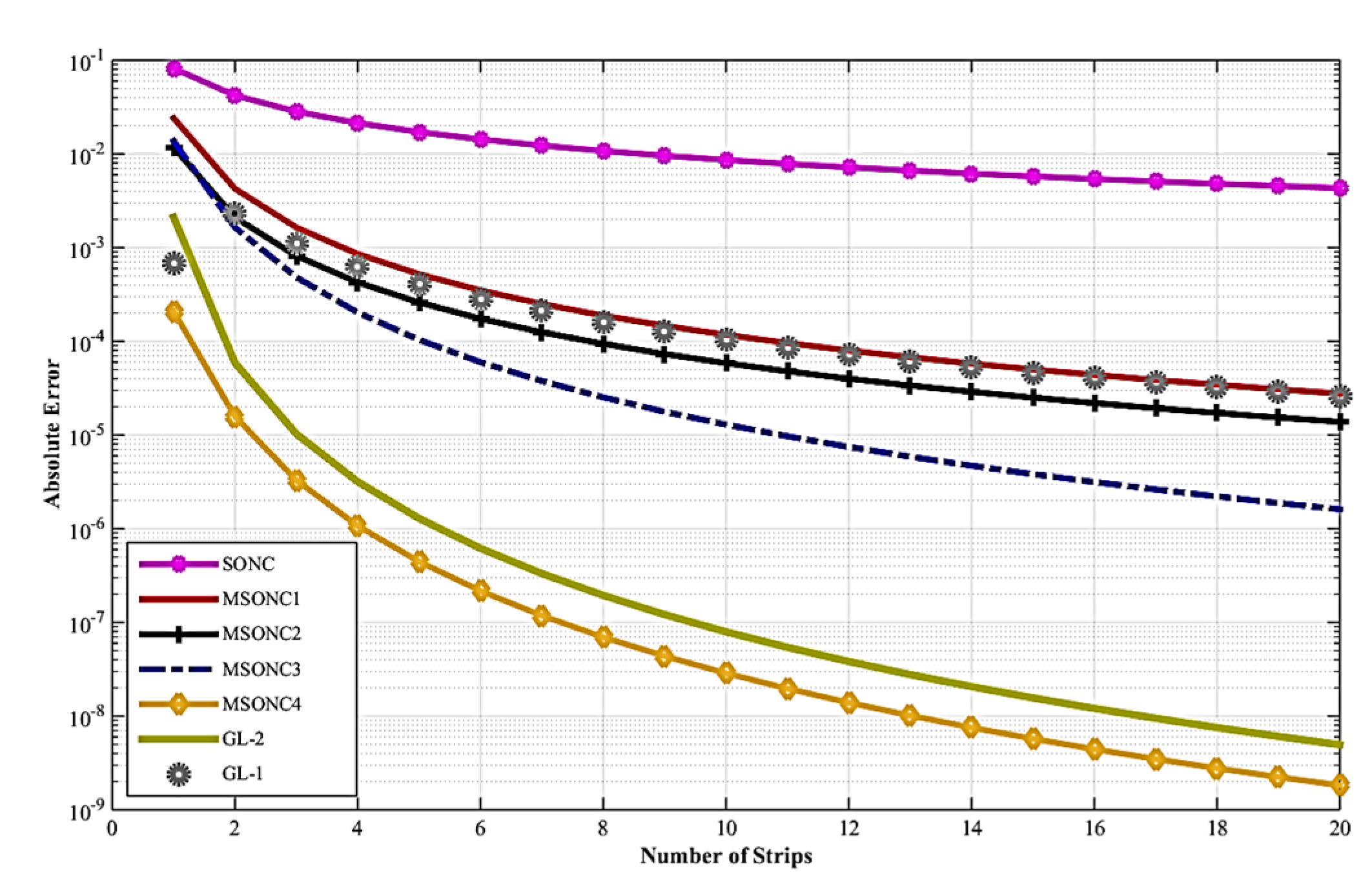
We compare the absolute error distributions versus the number of strips between the new and conventional approaches. The following formula is used to examine the absolute errors [1].

$$\mathrm{Absolute} \mathrm{Error}=\left|f^{*}\left(x\right)-f\left(x\right)\right|$$

(63)

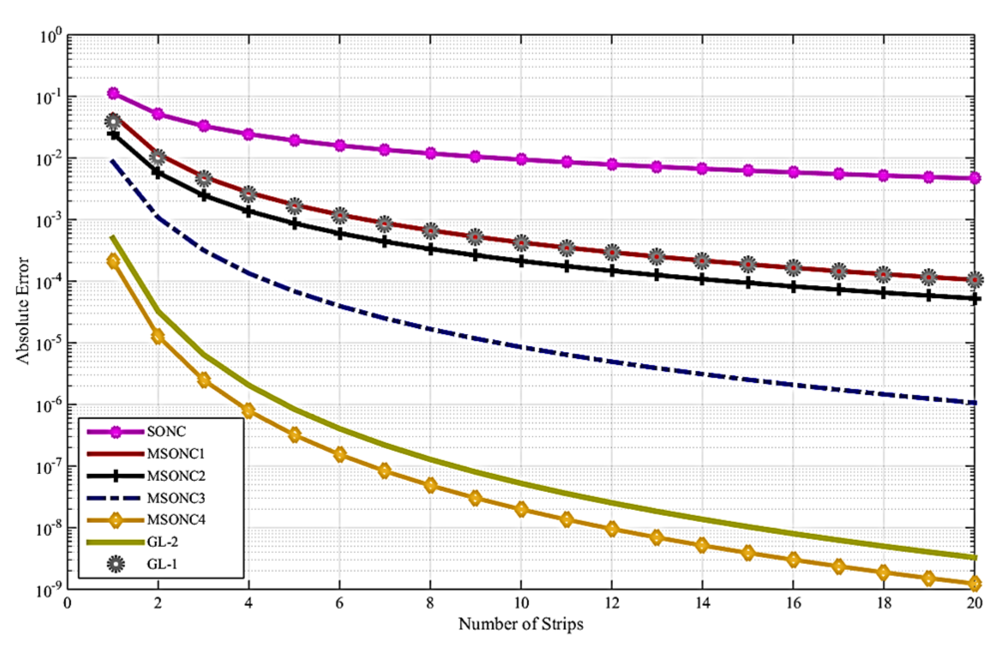
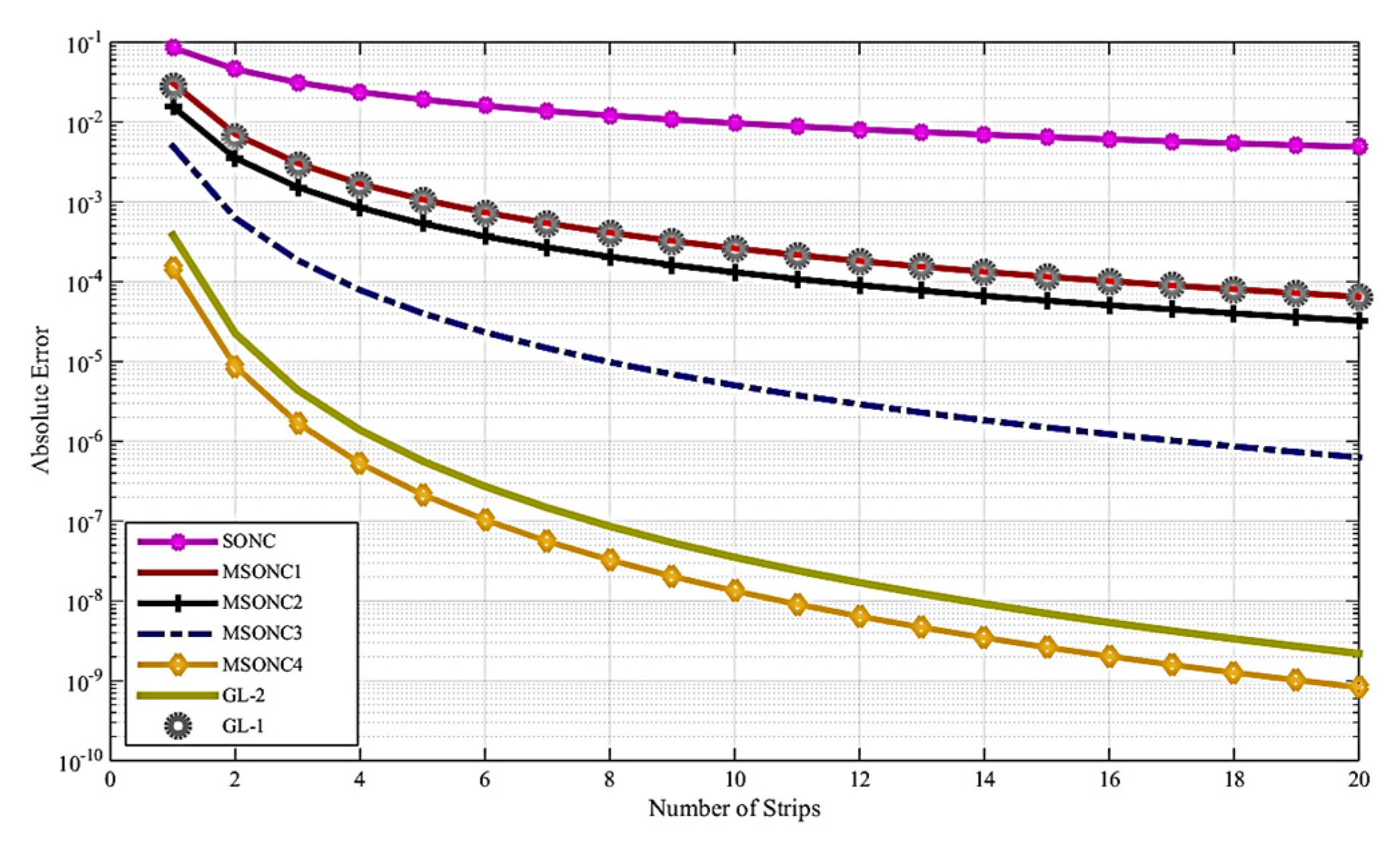
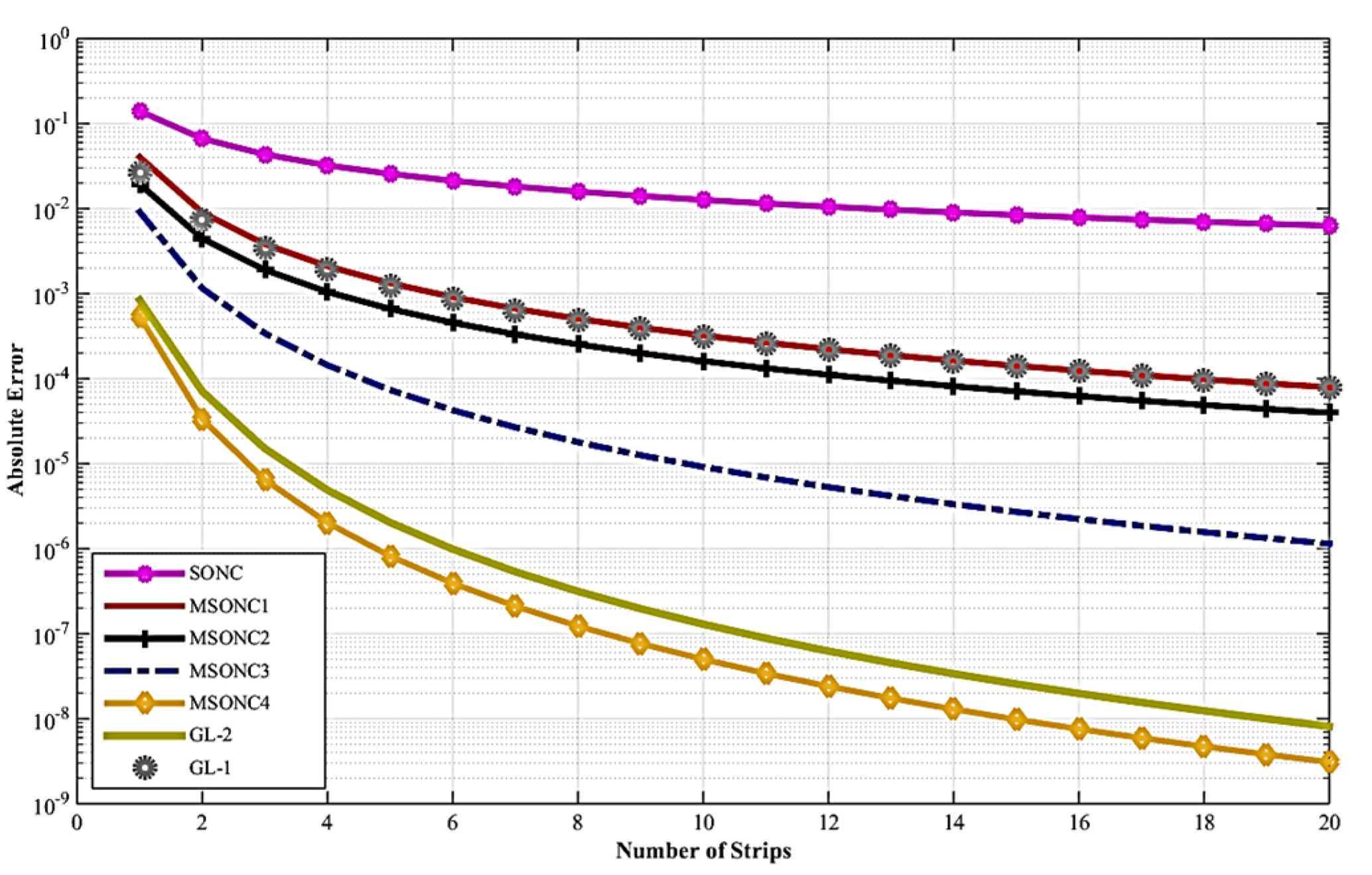
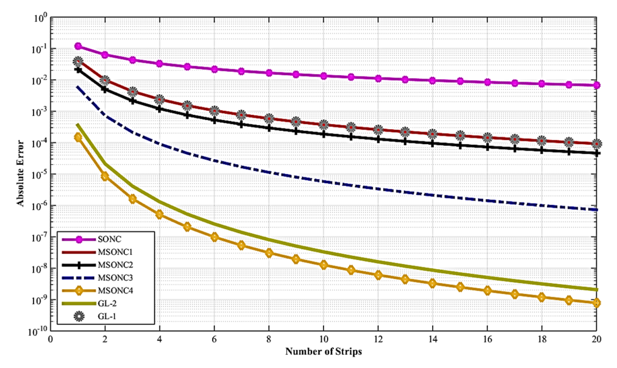
where, $f^{*}\left(x\right)$ and $f\left(x\right)$ represents the exact and approximate values (obtained by proposed methods) of the integrand. Figure 1, Figure 2, Figure 3, Figure 4 and Figure 5 represent the absolute errors that are calculated to examine and compare the results of the classical SONC, GL1, GL2, and modified derivative-based SONC methods and MSONC1–4 versus the number of strips for the first five integrals mentioned above. Hence, these figures show the decreasing absolute error distributions for all the integrals and the trends depict the faster convergence of the proposed methods, and the order of accuracy is consistent with the derived error terms. The outcomes generated by the new methods confirm that these possess lower errors than the original ones. Particularly, the MSONC4 behaves best of all, even the accompanying GL2 rule with similar order of accuracy (4). 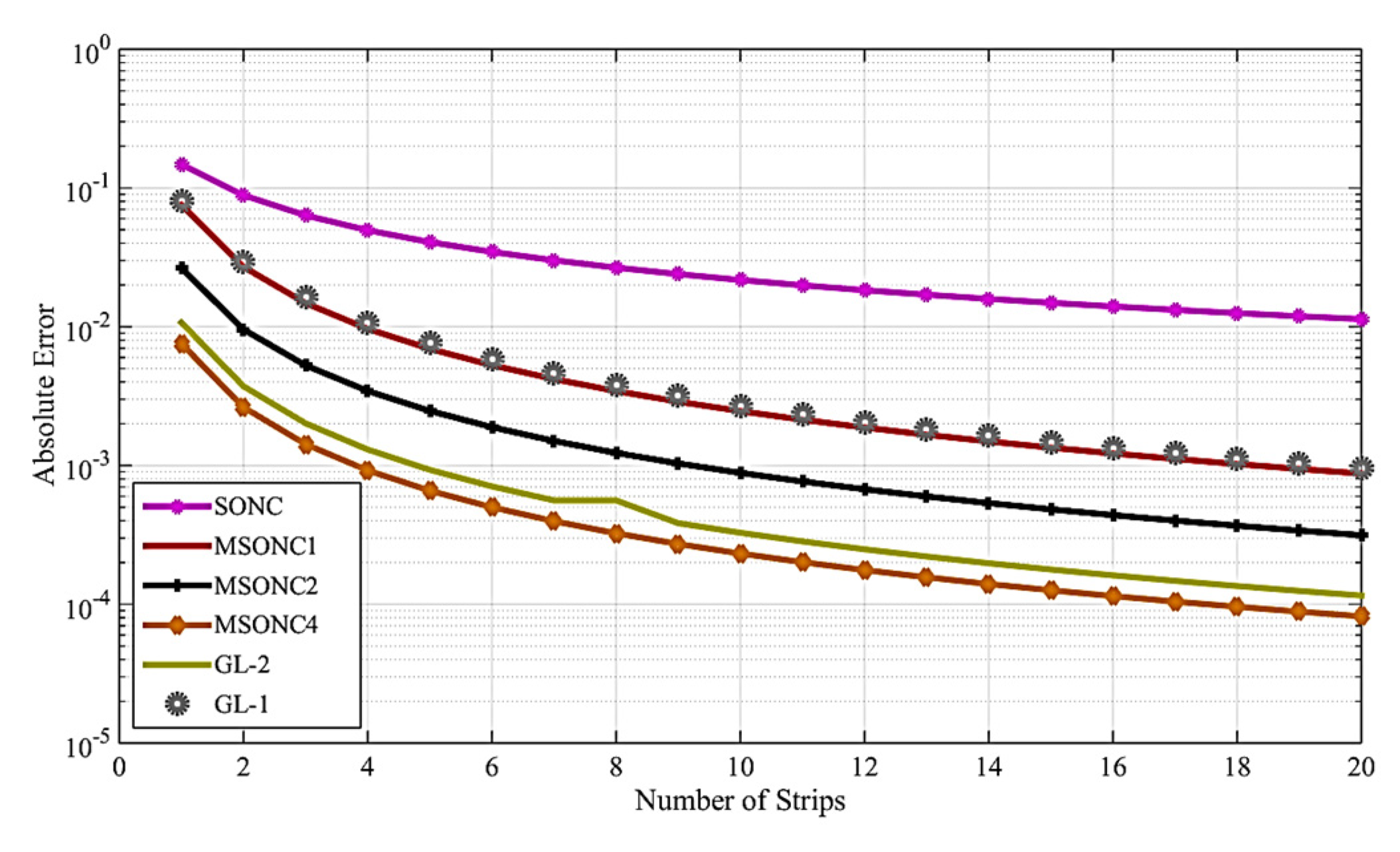Whereas the MSONC2 and 3 are better than SONC and GL1 rules. 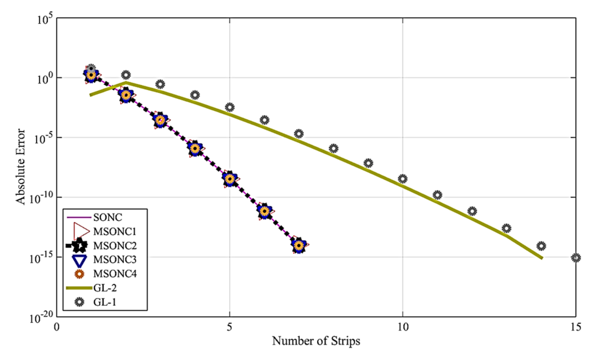For Example 6 through Figure 6, which is with a derivative singularity of the integrand, all applicable proposed methods continue the similar improvement and exhibit lower absolute errors as strips increase against respective derivative-free SONC, GL1 and GL2 rules. For the periodic integrals of Examples 7 and 8, the error drops from Figure 7 and Figure 8 confirm that the proposed MSONC1–4 and the conventional SONC rules show much-accelerated convergence than what is theoretically expected and achieve double precision accuracy quickly in fewer strips as compared to the GL1 and GL2 rules. This is due to the fact that Newton–Cotes rules and consequent improvements are more suitable for the periodic integrals than other methods utilizing zeros of orthogonal polynomials as nodes. 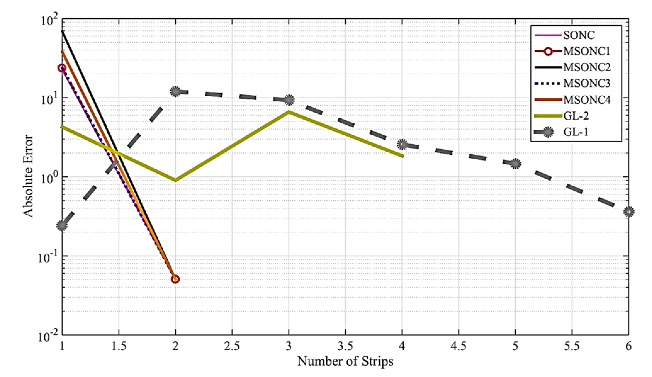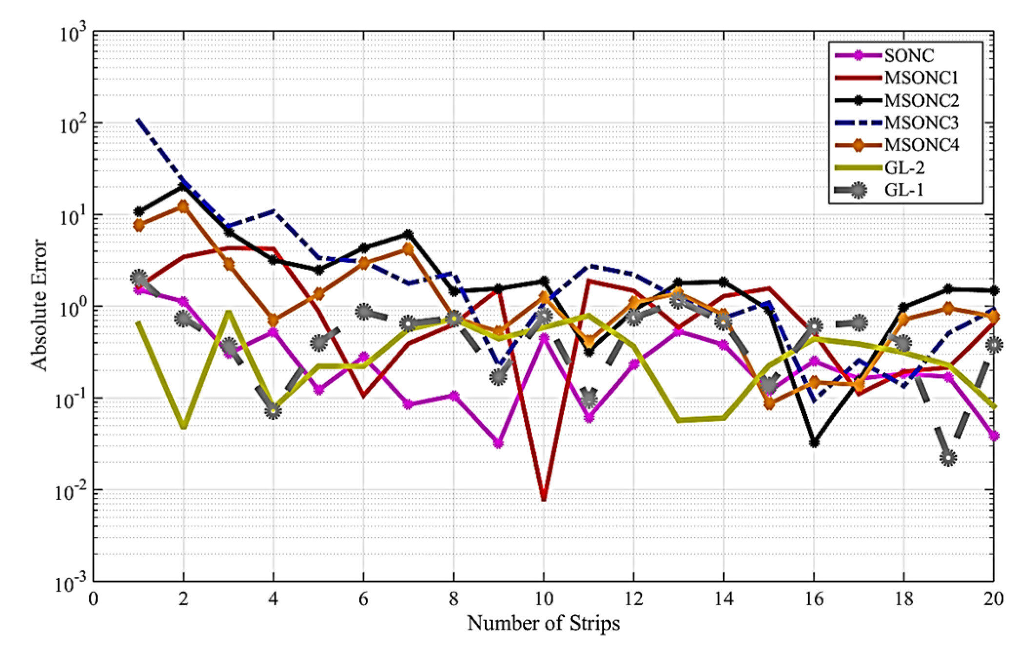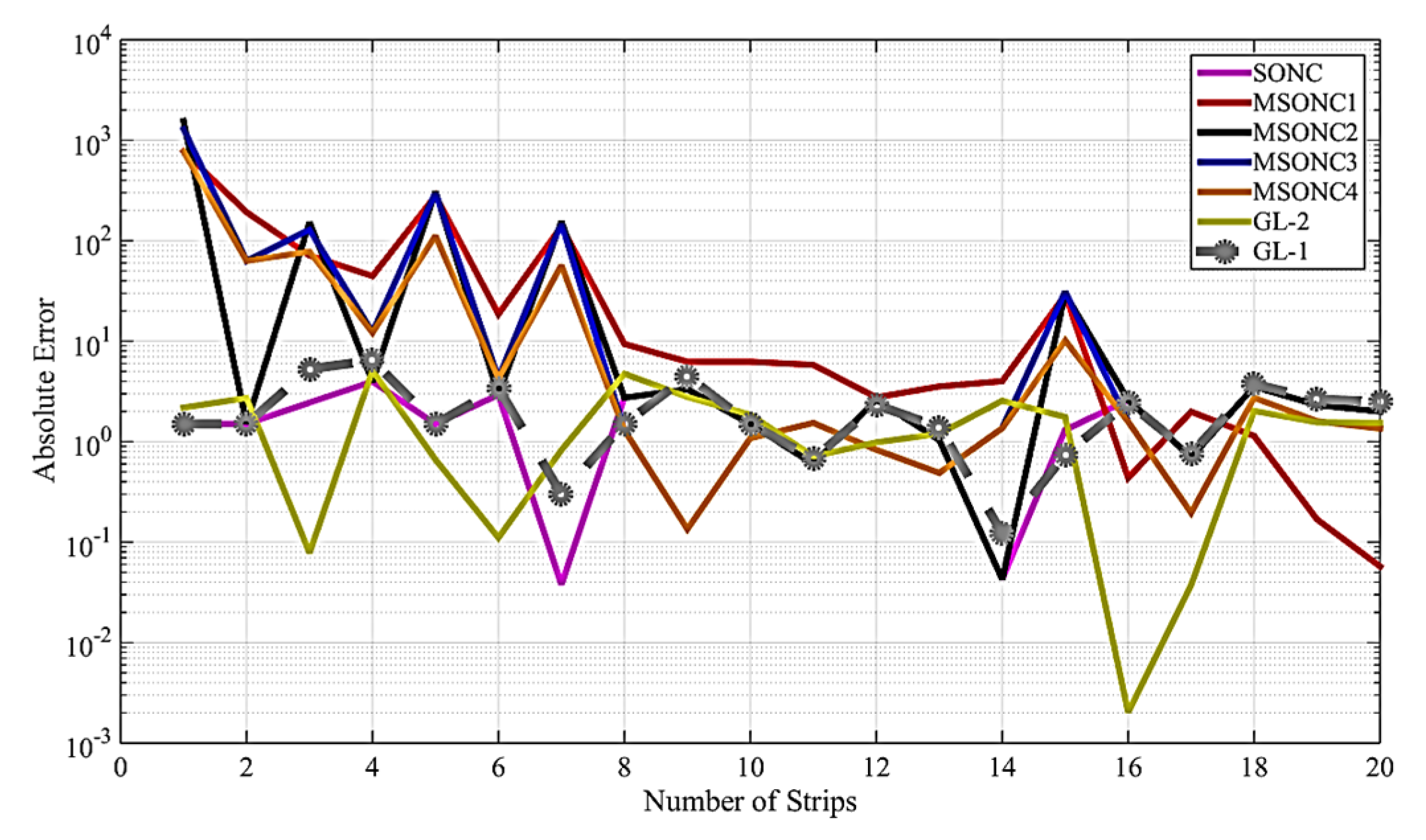Figure 9 and Figure 10 show an oscillatory pattern of error drops for approximating integrals in Examples 9 and 10 by all methods as expected. However, the higher order methods, without any specification that they use derivatives or not, try to hit lower errors alternatively. The MSONC4 and GL2 behave in this way better than other methods in Examples 9 and 10, respectively. These last two examples highlight the fact that when integrands are highly nonlinear and oscillatory, the decreasing error patterns are not that smooth and stable; however, all interpolatory quadrature methods have to compromise on accuracy regardless of the use of derivatives.

Finally, the total computational cost per integration step is observed to achieve the pre-specified error tolerance, i.e., $1\times {10}^{-7}$ mostly in regular examples, whereas bit lower in complicated integrals, and the average C.P.U time (in seconds) is also computed. Due to the higher number of function evaluations at each integration step, a quadrature rule might provide reasonable accuracy in fewer steps but could also be computationally more expensive and less effective than other approaches. First, the computational costs are determined for the methods generally in

Table 11. Computational costs for $m-\mathrm{strips}$ of all methods.

$\mathbf{M}\mathbf{e}\mathbf{t}\mathbf{h}\mathbf{o}\mathbf{d}\mathbf{s}$	$\mathbf{T}\mathbf{o}\mathbf{t}\mathbf{a}\mathbf{l}$
$SONC$	$m$
$MSONC1$	$2m$
$MSONC2$	$2m$
$MSONC3$	$2m+1$
$MSONC4$	$3m$
GL-1	$m$
GL-2	$2m$

as the total evaluations required per strip summarized for the modified and existing methods, by which we found the computational costs of each test problem. In

Table 12. Computational costs comparison to achieve $1\times {10}^{-7}$ absolute error for Examples 1–6.

$\mathbf{M}\mathbf{e}\mathbf{t}\mathbf{h}\mathbf{o}\mathbf{d}\mathbf{s}$	$\mathbf{E}\mathbf{x}\mathbf{a}\mathbf{m}\mathbf{p}\mathbf{l}\mathbf{e} \mathbf{1}$	$\mathbf{E}\mathbf{x}\mathbf{a}\mathbf{m}\mathbf{p}\mathbf{l}\mathbf{e} \mathbf{2}$	$\mathbf{E}\mathbf{x}\mathbf{a}\mathbf{m}\mathbf{p}\mathbf{l}\mathbf{e} \mathbf{3}$	$\mathbf{E}\mathbf{x}\mathbf{a}\mathbf{m}\mathbf{p}\mathbf{l}\mathbf{e} \mathbf{4}$	$\mathbf{E}\mathbf{x}\mathbf{a}\mathbf{m}\mathbf{p}\mathbf{l}\mathbf{e} \mathbf{5}$	$\mathbf{E}\mathbf{x}\mathbf{a}\mathbf{m}\mathbf{p}\mathbf{l}\mathbf{e} \mathbf{6}$
$SONC$	919,698	981,747	1,250,000	1,360,000	3,465,800	500,000
$MSONC1$	1290	1014	1118	1214	646	8516
$MSONC2$	912	718	792	860	456	4313
$MSONC3$	87	75	93	79	101	NA
$MSONC4$	18	21	27	18	21	1748
GL-1	1292	1016	1120	1216	648	18,104
GL-2	16	14	20	14	18	4380

and

Table 13. Computational costs comparison to achieve $1\times {10}^{-15}$ (Examples 7 and 8) and $1\times {10}^{-1}$ (Examples 9 and 10).

$\mathbf{M}\mathbf{e}\mathbf{t}\mathbf{h}\mathbf{o}\mathbf{d}\mathbf{s}$	$\mathbf{E}\mathbf{x}\mathbf{a}\mathbf{m}\mathbf{p}\mathbf{l}\mathbf{e} \mathbf{7}$	$\mathbf{E}\mathbf{x}\mathbf{a}\mathbf{m}\mathbf{p}\mathbf{l}\mathbf{e} \mathbf{8}$	$\mathbf{E}\mathbf{x}\mathbf{a}\mathbf{m}\mathbf{p}\mathbf{l}\mathbf{e} \mathbf{9}$	$\mathbf{E}\mathbf{x}\mathbf{a}\mathbf{m}\mathbf{p}\mathbf{l}\mathbf{e} \mathbf{10}$
SONC	7	3	7	7
$MSONC1$	7	3	8	16
MSONC2	7	3	10	11
$MSONC3$	7	3	9	9
$MSONC4$	7	3	4	9
GL-1	15	6	4	14
GL-2	14	18	4	4

, we list the total computational cost for the integrals mentioned in Examples 1–6 and Examples 7–10, respectively. It is analyzed from the numerical results that the computational cost of the proposed MSONC1–4 methods is lesser than the conventional SONC and GL-1 methods for examples 1–5, whereas the MSONC-4 and GL-2 methods are computationally closer in performance with GL-2 taking a slight edge over the MSONC4. It should be noted that the error drops of the MSONC4 over shown to be smaller than those of GL-2 in similar examples through Figure 1, Figure 2, Figure 3, Figure 4 and Figure 5. Thus, the proposed methods are cost-effective as compared to the conventional ones and MSONC4 competes well with the GL-2 rule which is a two-point method and the MSONC4 is a one-point method. For Example 6, the MSONC1,2,4 exhibit cost-efficient behavior from Table 12 against all derivative-free methods SONC and GL-1,2. Here, MSONC4 is best of all computationally for the integral with derivative singularity. All the SONC versions, existing derivative-free as well as the proposed derivative-based MSONC1–4 out-perform in comparison to the GL-1,2 rules for periodic integrals in Examples 7 and 8 from the viewpoint of achieving the double precision accuracy in lesser cost as shown in Table 13. For the oscillatory integrals of Examples 9 and 10 through Table 13, one can see that the SONC, GL-2 and the MSONC1–4 show similar performance with the GL-2 and MSONC4 taking the edge over others to achieve one decimal place accuracy. However, for higher accuracy, all methods continue showing oscillatory error drops as shown in Figure 9 and Figure 10 already.

After computational ascendance in terms of computational costs to achieve a preset error of at most $1\times {10}^{-7}$ in regular examples and slightly lower in some, we now explore the execution times as CPU times (in seconds), which are used to determine the runtime of the processor in MATLAB software for each code of the method separately to meet up the preset accuracy level. The execution times account for all evaluations: derivative as well as functional ones to finally determine the time efficiency of the methods. A salient feature to examine the execution times is to explore the concern of whether the proposed rules with derivatives add much more burden on the processor based on the fact that derivatives may sometimes be more complex in computation than the functions alone. We noted already that the proposed quadrature formulas use a lower total number of evaluations (functional as well as derivative) compared to the SONC and some other conventional rules without derivatives in form of computational costs. The execution time helps us in proving that the amount of processing power required for functional, as well as some derivative evaluations in the proposed quadrature formulas, is not a big compromise as that required by the conventional rules with only a lot of functional evaluations.

Table 14. Average CPU time (in seconds) comparison to achieve $1\times {10}^{-7}$ absolute error for Examples 1–6.

$\mathbf{M}\mathbf{e}\mathbf{t}\mathbf{h}\mathbf{o}\mathbf{d}\mathbf{s}$	$\mathbf{E}\mathbf{x}\mathbf{a}\mathbf{m}\mathbf{p}\mathbf{l}\mathbf{e} \mathbf{1}$	$\mathbf{E}\mathbf{x}\mathbf{a}\mathbf{m}\mathbf{p}\mathbf{l}\mathbf{e} \mathbf{2}$	$\mathbf{E}\mathbf{x}\mathbf{a}\mathbf{m}\mathbf{p}\mathbf{l}\mathbf{e} \mathbf{3}$	$\mathbf{E}\mathbf{x}\mathbf{a}\mathbf{m}\mathbf{p}\mathbf{l}\mathbf{e} \mathbf{4}$	$\mathbf{E}\mathbf{x}\mathbf{a}\mathbf{m}\mathbf{p}\mathbf{l}\mathbf{e} \mathbf{5}$	$\mathbf{E}\mathbf{x}\mathbf{a}\mathbf{m}\mathbf{p}\mathbf{l}\mathbf{e} \mathbf{6}$
$SONC$	1.0190	1.0238	0.8856	1.0461	20.5804	140.08610
$MSONC1$	0.1623	0.1619	0.1074	0.1561	0.2571	3.07367
$MSONC2$	0.4316	0.4432	0.2968	0.4175	0.5388	1.8850
$MSONC3$	0.4229	0.4184	0.2976	0.4215	0.5191	NA
$MSONC4$	0.4360	0.4371	0.3180	0.4162	0.5442	1.3438
GL-1	0.5945	0.5055	0.5897	0.5470	0.7102	1.7778
GL-2	0.4524	0.4299	0.4288	0.4176	0.5424	1.7599

and

Table 15. Average CPU time (in seconds) comparison to achieve $1\times {10}^{-2}$ absolute error for Examples 7–10.

$\mathbf{M}\mathbf{e}\mathbf{t}\mathbf{h}\mathbf{o}\mathbf{d}\mathbf{s}$	$\mathbf{E}\mathbf{x}\mathbf{a}\mathbf{m}\mathbf{p}\mathbf{l}\mathbf{e} \mathbf{7}$	$\mathbf{E}\mathbf{x}\mathbf{a}\mathbf{m}\mathbf{p}\mathbf{l}\mathbf{e} \mathbf{8}$	$\mathbf{E}\mathbf{x}\mathbf{a}\mathbf{m}\mathbf{p}\mathbf{l}\mathbf{e} \mathbf{9}$	$\mathbf{E}\mathbf{x}\mathbf{a}\mathbf{m}\mathbf{p}\mathbf{l}\mathbf{e} \mathbf{10}$
$SONC$	1.1232	2.4760	1.7046	1.9635
$MSONC1$	1.0804	2.5746	1.7105	1.5916
$MSONC2$	1.2569	2.5071	1.7613	1.9557
$MSONC3$	1.1261	2.4570	1.5616	1.8320
$MSONC4$	1.2377	2.4157	1.6502	1.8456
GL-1	1.2034	2.6656	1.8347	1.9282
GL-2	1.1181	2.0629	1.6647	1.8177

list the CPU times (in seconds) for all methods in the case of Examples 1–6 and 7–10, respectively. We observe that in this sense as well, the proposed formulas take ascendancy over the existing derivative-free one-point methods: SONC and GL-1. For the two-point GL-2 method, the results by the proposed MSONC1–4 compare well and are mostly lower in some instances. Additionally, the average CPU time achieved by the new techniques is smaller than the average CPU time of the original SONC method and comparable with the GL-1,2 rules, which utilize special nodes at the zeros of Legendre polynomials, to achieve the same error. Thus, the proposed methods are time efficient as well and the numerical evidence suggests that the execution times for the derivatives are not as high as for the usual nodes.

5. Conclusions

In this research, four efficient quadrature formulas using derivatives to compute integrals have been proposed, which were computationally efficient, cost-effective and time-efficient modifications of the conventional semi-open Newton–Cotes quadrature rule. The theoretical development of the methods along with theorems with proofs on the order of accuracy, degree of precision and error terms for all the proposed methods were discussed. An exhaustive comparison was carried out on several integrals from the literature involving regular, periodic and derivative-singular and oscillatory integrands. In addition to this, computational results in terms of computational cost, observed orders of accuracy, average C.P.U times (in seconds), as well as absolute error drops, were also determined for ten test integrals from literature to compare all proposed methods with derivatives MSONC1, MSONC2, MSONC3, and MSONC4 with classical derivative-free SONC and GL-1, GL-2 rules. The analysis of the results depicts the efficiency of the modified methods over the conventional methods. The main features have been the cost-effectiveness and time efficiency of the proposed methods with derivatives with enhanced theoretical properties over the existing derivative-free methods not only in regular integrals but also in the case of some special integrals.

References

1. Chapra, S.C. Applied Numerical Methods with MATLAB, 3rd ed.; Mc Graw Hill Education Private Ltd.: New Delhi, India, 2012; pp. 103–106. [Google Scholar]
2. Atkinson, K. An Introduction to Numerical Analysis. In Interpolation Theory, 2nd ed.; John Wiley & Sons: New York, NY, USA, 1988; p. 170. [Google Scholar]
3. Shaikh, M.M. Analysis of Polynomial Collocation and Uniformly Spaced Quadrature Methods for Second Kind Linear Fredholm Integral Equations—A Comparison. Turk. J. Anal. Number Theory 2019, 7, 91–97. [Google Scholar]
4. Zafar, F.; Saleem, S.; Burg, C.O.E. New Derivative Based Open Newton-Cotes Quadrature Rules. Abstr. Appl. Anal. 2014, 2014, 109138. [Google Scholar] [CrossRef]
5. El-Mikkawy, M. A unified approach to Newton–Cotes quadrature formulae. Appl. Math. Comput. 2003, 138, 403–413. [Google Scholar] [CrossRef]
6. El-Mikkawy, M.E.A. On the Error Analysis Associated with the Newton-Cotes Formulae. Int. J. Comput. Math. 2002, 79, 1043–1047. [Google Scholar] [CrossRef]
7. Dehghan, M.; Masjed-Jamei, M.; Eslahchi, M. On numerical improvement of closed Newton–Cotes quadrature rules. Appl. Math. Comput. 2004, 165, 251–260. [Google Scholar] [CrossRef]
8. Dehghan, M.; Masjed-Jamei, M.; Eslahchi, M. On numerical improvement of open Newton–Cotes quadrature rules. Appl. Math. Comput. 2006, 175, 618–627. [Google Scholar] [CrossRef]
9. Dehghan, M.; Masjed-Jamei, M.; Eslahchi, M. The semi-open Newton–Cotes quadrature rule and its numerical improvement. Appl. Math. Comput. 2005, 171, 1129–1140. [Google Scholar] [CrossRef]
10. Hashemiparast, S.; Eslahchi, M.; Dehghan, M.; Masjed-Jamei, M. The first kind Chebyshev–Newton–Cotes quadrature rules (semi-open type) and its numerical improvement. Appl. Math. Comput. 2006, 174, 1020–1032. [Google Scholar] [CrossRef]
11. Hashemiparast, S.M.; Masjed-Jamei, M.; Eslahchi, M.R.; Dehghan, M. The second kind Chebyshev-Newton-Cotes quadraturerule (open type) and its numerical improvement. Appl. Math. Comput. 2006, 180, 605–613. [Google Scholar] [CrossRef]
12. Clarence, O.E.; Burg, C.O. Derivative-based closed Newton–Cotes numerical quadrature. Appl. Math. Comput. 2012, 218, 7052–7065. [Google Scholar] [CrossRef]
13. Clarence, O.E.; Degny, E. Derivative-Based Midpoint Quadrature Rule. Appl. Math. 2013, 04, 228–234. [Google Scholar] [CrossRef]
14. Zhao, W.; Li, H. Midpoint Derivative-Based Closed Newton-Cotes Quadrature. Abstr. Appl. Anal. 2013, 2013, 492507. [Google Scholar] [CrossRef] [Green Version]
15. Zhao, W.; Zhang, Z. Derivative-Based Trapezoid Rule for the Riemann-Stieltjes Integral. Math. Probl. Eng. 2014, 2014, 874651. [Google Scholar] [CrossRef] [Green Version]
16. Memon, K.; Shaikh, M.; Chandio, M.; Shaikh, A. A Modified Derivative-Based Scheme for the Riemann-Stieltjes Integral. SINDH Univ. Res. J.-Sci. Ser. 2020, 52, 37–40. [Google Scholar] [CrossRef]
17. Memon, K.; Shaikh, M.M.; Chandio, M.S.; Shaikh, A.W. An Efficient Four-point Quadrature Rule for Reimann Stieljes Integral. J. Mech. Contin. Math. Sci. 2021, 16, 2454–7190. [Google Scholar] [CrossRef]
18. Malik, K.; Shaikh, M.M.; Chandio, M.S.; Shaikh, A.W. Error Analysis of Newton Cotes Cubature Rulesl. J. Mech. Contin. Math. Sci. 2020, 15, 2454–7190. [Google Scholar]
19. Billingsley, P. Probability and Measures; John Wiley and Sons, Inc.: New York, NY, USA, 1995. [Google Scholar]
20. Egghe, L. Construction of concentration measures for General Lorenz curves using Riemann-Stieltjes integrals. Math. Comput. Model. 2002, 35, 1149–1163. [Google Scholar] [CrossRef] [Green Version]
21. Rossberg, H.-J. Kopp, P.E., Martingales and Stochastic Integrals. Cambridge et al., Cambridge University Press 1984. XI, 202 S., £ 17.50 B H/c. US $ 29.95. ISBN 0-521-24758-6. J. Appl. Math. Mech./Z. Angew. Math. Mech. 1985, 65, 536. [Google Scholar] [CrossRef]
22. D’Ambrosio, R.; Scalone, C. Filon quadrature for stochastic oscillators driven by time-varying forces. Appl. Numer. Math. 2021, 169, 21–31. [Google Scholar] [CrossRef]
23. D’Ambrosio, R.; Scalone, C. Asymptotic Quadrature Based Numerical Integration of Stochastic Damped Oscillators. In Proceedings of the ICCSA 2021: Computational Science and Its Applications, Cagliari, Italy, 13–16 September 2021; 12950 LNCS. pp. 622–629. [Google Scholar]
24. Rudin, W. Functional Analysis; McGraw Hill Science: New York, NY, USA, 1991. [Google Scholar]
25. Kanwal, R.P. Linear Integral Equations; Academic Press, Inc.: California, CA, USA; Elsevier: Amsterdam, The Netherlands, 1971; pp. 167–193. [Google Scholar] [CrossRef]
26. Iserles, A.; Nørsett, S.P. Efficient quadrature of highly oscillatory integrals using derivatives. Proc. R. Soc. A Math. Phys. Eng. Sci. 2005, 461, 1383–1399. [Google Scholar] [CrossRef] [Green Version]
27. Iserles, A.; Nørsett, S.P. On Quadrature Methods for Highly Oscillatory Integrals and Their Implementation. BIT Numer. Math. 2004, 44, 755–772. [Google Scholar] [CrossRef]
28. Khanamiryan, M. Quadrature methods for highly oscillatory linear and nonlinear systems of ordinary differential equations: Part I. BIT Numer. Math. 2008, 48, 743–761. [Google Scholar] [CrossRef]
29. Dahlquist, G.; Björck, Å. Numerical Methods; Courier Corporation: Chelmsford, MA, USA, 2003. [Google Scholar]
30. Trefethen, L.N.; Weideman, J.A.C. The exponentially convergent Trapezoidal rule. SIAM Rev. 2014, 56, 385–458. [Google Scholar] [CrossRef] [Green Version]
31. Ramachandran, T.; Parimala, R. Open Newton cotes quadrature with midpoint derivative for integration of Algebraic functions. Int. J. Res. Eng. Technol. 2015, 4, 430–435. [Google Scholar] [CrossRef]
32. Ramachandran, T.; Udayakumar, D.; Parimala, R. Geometric mean derivative-based closed Newton cotes quadrature. Int. J. Pure Eng. Math. 2016, 4, 107–116. [Google Scholar]
33. Ramachandran, T.; Udayakumar, D.; Parimala, R. Comparison of Arithmetic Mean, Geometric Mean and Harmonic Mean Derivative-Based Closed Newton Cotes Quadrature. Prog. Nonlinear Dyn. Chaos 2016, 4, 35–43. [Google Scholar]
34. Ramachandran, T.; Parimala, R. Centroidal Mean Derivative-Based Closed Newton Cotes Quadrature. Int. J. Sci. Res. 2016, 5, 338–343. [Google Scholar]
35. Rana, K. Harmonic Mean and Contra-Harmonic Mean Derivative-Based Closed Newton-Cotes Quadrature. Integr. J. Res. Arts Humanit. 2022, 2, 55–61. [Google Scholar] [CrossRef]
36. Ramachandran, T.; Udayakumar, D.; Parimala, R. Heronian mean derivative-based closed newton cotes quadrature. Int. J. Math. Arch. 2016, 7, 53–58. [Google Scholar]
37. Marjulisa, R.; Imran, M. Syamsudhuha Arithmetic mean derivative based midpoint rule. Appl. Math. Sci. 2018, 12, 625–633. [Google Scholar] [CrossRef] [Green Version]
38. Ehrenmark, U.T. A three-point formula for numerical quadrature of oscillatory integrals with variable frequency. J. Comput. Appl. Math. 1988, 21, 87–99. [Google Scholar] [CrossRef]
Figure 1. Absolute error drops versus number of strips for Example 1.
Symmetry 14 02611 g001
Figure 2. Absolute error drops versus number of strips for Example 2.
Symmetry 14 02611 g002
Figure 3. Absolute error drops versus number of strips for Example 3.
Symmetry 14 02611 g003
Figure 4. Absolute error drops versus number of strips for Example 4.
Symmetry 14 02611 g004
Figure 5. Absolute error drops versus number of strips for Example 5.
Symmetry 14 02611 g005
Figure 6. Absolute error drops versus number of strips for Example 6.
Symmetry 14 02611 g006
Figure 7. Absolute error drops versus number of strips for Example 7.
Symmetry 14 02611 g007
Figure 8. Absolute error drops versus number of strips for Example 8.
Symmetry 14 02611 g008
Figure 9. Absolute error drops versus number of strips for Example 9.
Symmetry 14 02611 g009
Figure 10. Absolute error drops versus number of strips for Example 10.
Symmetry 14 02611 g010