Article

Measurement of the Central Galactic Black Hole by Extremely Large Mass-Ratio Inspirals

1
Shanghai Astronomical Observatory, Chinese Academy of Sciences, Shanghai 200030, China
2
School of Fundamental Physics and Mathematical Sciences, Hangzhou Institute for Advanced Study, UCAS, Hangzhou 310024, China
3
University of Chinese Academy of Sciences (UCAS), Beijing 100049, China
*
Author to whom correspondence should be addressed.
Symmetry 2022, 14(12), 2558; https://doi.org/10.3390/sym14122558
Submission received: 29 September 2022 / Revised: 14 November 2022 / Accepted: 30 November 2022 / Published: 3 December 2022
(This article belongs to the Special Issue Symmetry in Gravity Research)

Abstract

:
In the galaxy, extremely large mass-ratio inspirals (X-MRIs) composed of brown dwarfs and the massive black hole at the galactic center are expected to be promising gravitational wave sources for space-borne detectors. In this work, we simulate the gravitational wave signals from twenty X-MRI systems by an axisymmetric Konoplya–Rezzolla–Zhidenko metric with varied parameters. We find that the mass, spin, and deviation parameters of the Kerr black hole can be determined accurately (∼ 10 5 10 6 ) with only one X-MRI event with a high signal-to-noise ratio. The measurement of the above parameters could be improved with more X-MRI observations.

1. Introduction

The first observations of gravitational waves (GWs) from binary black hole mergers and binary neutron star inspirals ushered in a new era of GW physics and astronomy [1,2]. Since then, the ground-based detectors have detected 90 GW events [3,4,5]. The detectable frequency band of current ground-based GW detectors such as Advanced LIGO [6], Advanced Virgo [7], and KAGRA [8] ranges from 10 to 10,000 Hz, which makes ground-based GW detectors unable to detect any GWs with frequencies less than 10 Hz, while abundant sources are emitting GWs in the low-frequency band [9]. The space-borne GW detectors such as LISA [10], Taiji [11], and TianQin [12], which will be launched in the 2030s, will open GW windows from 0.1 mHz to 1 Hz and are expected to probe the nature of astrophysics, cosmology, and fundamental physics.
One of the most essential and promising GW sources for space-borne GW detectors is the extreme-mass ratio inspiral (EMRI), which is formed when a massive black hole (MBH) captures a small compact object [9,13]. The word “inspiral” here means the inspiralling process such that the relatively lighter object gradually spirals in toward the MBH due to the emission of GWs. The small object should be compact to keep it from being tidally disrupted by the MBH so that it is unlikely to be a main-sequence star. The possible candidate could be a stellar-mass black hole(BH), neutron star, white dwarf, or other compact object. The designed space-borne detectors will be sensitive to EMRIs that contain MBHs with the mass 10 4 10 7 M and small compact objects with stellar mass, and the fiducial mass ratio will be 10 3 10 6 [14].
Moreover, a special kind of EMRI, extremely large mass-ratio inspirals (X-MRIs) with a mass ratio of q 10 8 are also potential sources for space-borne GW detectors [15,16]. An X-MRI system is formed when an MBH captures a brown dwarf (BD) with a mass of ∼ 10 2 M . Brown dwarfs are substellar objects with insufficient mass to sustain nuclear fusion and become main-sequence stars [17]. Brown dwarfs are denser than main-sequence stars, and their Roche limit is closer to the horizon of MBH [15,18]. Therefore, brown dwarfs could survive very close to the MBH.
The mass of BD is relatively tiny, so space-borne GW detectors such as LISA could only observe X-MRIs nearby, especially X-MRIs at the galactic center(GC) [15,16]. The MBH of these X-MRIs, Sgr A*, is 8 kpc from the solar system, and its mass is about 4 × 10 6 M [19,20,21,22]. A typical X-MRI at the GC covers ∼ 10 8 cycles, which last millions of years in the LISA band [16]. Such an X-MRI could have a relatively high SNR (more than 1000), and dozens of X-MRIs might be observed during the LISA mission period [16]. Therefore, the X-MRIs at the GC offers a natural laboratory for studying the properties of BH and testing theories of gravity.
In this paper, we simulate the GW signals of X-MRIs at the GC to show how and to what extent the fine structure of Sgr A* could be figured. In general relativity (GR), according to the no-hair theorem, BHs are characterized by their masses, spins, and electric charges, and the Kerr metric is believed to be the metric that describes the space-time of BH. However, alternative theories of gravity predict hairy black holes [23] and other metrics that describe the space-time of BH [24]. The parameterized metrics are proposed to describe the space-time of non-Kerr black holes. In this paper, to describe the space-time of X-MRIs at the GC, we use a model-independent parameterization metric, the Konoplya–Rezzolla–Zhidenko metric (KRZ metric) [24], which can describe metrics that are generic stationary and axisymmetric.
This paper is organized as follows. In Section 2, we review the KRZ parametrization. In Section 3, we introduce the “kludge” waveforms used in our work and simulate the GW signals emitted by X-MRIs at GC. In Section 4, based on the simulated GW signals, we apply the Fisher matrix to these GWs and present the accuracy of parameter estimation of Sgr A* for future space-borne GW detectors. The conclusion and outlook are given in Section 5. Throughout this letter, we use natural units ( G = c = 1 ) . Greek letters ( μ , ν , σ , ) stand for space-time indices, and Einstein summation is assumed.

2. KRZ Prametrized Metric

GR is the most accurate and concise theory of gravity by far [25]. In practice, there are quite a few other theories of gravity, whose predictions resemble general relativity’s, to be tested. In the framework of GR, the Schwarzschild or Kerr metric describes the space-time of an uncharged BH. However, in modified and alternative theories of gravity, there are other possible solutions for the description of the space-time of BHs [26,27,28,29,30,31]. The predictions of different theories of gravity are different, so a universal and reasonable theory about the GWs of an X-MRI should be model-independent.
In order to deal with the numerous metrics of non-Kerr black holes, one may use the parameterized metric to describe the space-time of non-Kerr black holes. There are several model-independent frameworks, one of which parametrizes the most generic black hole geometry through a finite number of adjustable quantities and is known as Johannsen–Psaltis parametrization (J-P metric) [32]. The J-P metric expresses deviations from general relativity in terms of a Taylor expansion in powers of M / r , where M is the mass of BH and r is the radial coordinate. The J-P parametrization is widely adopted, but it is not a robust and generic parametrization for rotating black holes [24,33]. Notably, the parametric axisymmetric J-P metric obtained from the Janis–Newman algorithm [34] does not cover all deviations from Kerr space-time.
Another model-independent parameterization metric [24,35], the KRZ metric, is based on a double expansion in both the polar and radial directions of a generic stationary and axisymmetric metric. The KRZ metric is effective in reproducing the space-time of three commonly used rotating black holes (Kerr, rotating dilation [36], and Einstein-dilaton-Gauss-Bonnet black holes [37]) with finite parameters (see Ref. [24] for more details). According to KRZ parameterization, the space-time of any axisymmetric black hole with total mass M and rotation parameter a could be expressed in the following form [24]:
d s 2 = N 2 W 2 sin 2 θ K 2 d t 2 2 W r sin 2 θ d t d ϕ + K 2 r 2 sin 2 θ d ϕ 2 + S B 2 N 2 d r 2 + r 2 d θ 2 ,
where [38]
S = Σ r 2 = 1 + a 2 r 2 cos 2 θ ,
Σ = r 2 + a 2 cos 2 θ ,
N , B , W , and K are the functions of the radial and polar coordinates (expanded in the term cos θ ),
W = i = 0 W i ( r ) ( cos θ ) i S ,
B = 1 + i = 0 B i ( r ) ( cos θ ) i ,
N 2 = 1 r 0 r A 0 ( r ) + i = 1 A i ( r ) ( cos θ ) i ,
K 2 = 1 + a W r + a 2 r 2 + i = 1 K i ( r ) ( cos θ ) i S ,
with
B i = b i 0 r 0 r + B i ˜ r 0 2 r 2 ,
B i ˜ b i 1 1 + x b i 2 1 + x b i 3 1 + . . . ,
W i = b i 0 r 0 2 r 2 + B i ˜ r 0 3 r 3 ,
W i ˜ ω i 1 1 + x ω i 2 1 + x ω i 3 1 + ,
K i > 0 ( r ) = k i 0 r 0 2 r 2 + K i ˜ r 0 3 r 3 ,
K i ˜ k i 1 1 + x k i 2 1 + x k i 3 1 + ,
A 0 ( r ) = 1 ϵ 0 r 0 r + ( a 00 ϵ ) r 0 2 r 2 + a 2 r 2 + A 0 ˜ r 0 3 r 3 ,
A i > 0 = K i ( r ) + ϵ i r 0 2 r 2 + a i 0 r 0 3 r 3 + A i ˜ r 0 4 r 4 ,
A i ˜ a i 1 1 + x a i 2 1 + x a i 3 1 + ,
where x = 1 r 0 / r , and r 0 is the radius of the black hole horizon in the equatorial plane. The metric (1) is characterized by the order of expansion in radial and polar directions. The parameters a i j , b i j , ω i j , k i j (here i = 0 , 1 , 2 , 3 , j = 1 , 2 , 3 ) are effectively independent. This is because one of these functions, A i ( x ) , B i ( x ) , W i ( x ) and K i ( x ) , is fixed by coordinate choice [38].
In the following, we present the parameterized metric with first-order radial expansion and second-order polar direction, which describe the space-time of a deformed Kerr black hole [33,38]:
B = 1 + δ 4 r 0 2 r 2 + δ 5 r 0 2 r 2 cos 2 θ ,
W = 1 Σ ω 00 r 0 2 r 2 + δ 2 r 0 3 r 3 + δ 3 r 0 3 r 3 cos 2 θ ,
K 2 = 1 + a W r + 1 Σ k 00 r 0 2 r 2 + k 21 r 0 3 r 3 cos 2 θ ,
N 2 = 1 r 0 r 1 ϵ 0 r 0 r + ( k 00 ϵ 0 ) r 0 2 r 2 + δ 1 r 0 3 r 3 + ( k 21 + a 20 ) r 0 3 r 3 + a 21 r 0 4 r 4 cos 2 θ ,
The radius of the horizon and the Kerr parameter are
r 0 = M + M 2 a 2 , a = J / M ,
where J is the total angular momentum. For simplicity, here, M has one unit, i.e., M = 1 . One can obtain related variables and parameters from a dimensionless quantity by scale transformations [39,40,41,42,43,44]: t M t , r M r , etc. The coefficient r 0 , a 20 , a 21 , ϵ 0 , k 00 , k 21 and ω 00 in the KRZ metric can be expressed as follows [33,45]
r 0 = 1 + 1 a ˜ 2 ,
a 20 = 2 a ˜ 2 r 0 3 ,
a 21 = a ˜ 4 r 0 4 + δ 6 ,
ϵ 0 = 2 r 0 r 0 ,
ω 00 = 2 a ˜ r 0 2 ,
k 00 = a ˜ 2 r 0 2 ,
k 21 = a ˜ 4 / r 0 4 2 a ˜ 2 / r 0 3 δ 6 ,
k 22 = a ˜ 2 / r 0 2 + δ 7 ,
k 23 = a ˜ 2 / r 0 2 + δ 8 ,
where a ˜ = a / M stands for the spin parameter. The deformation parameters δ j ( j = 1 , 2 , , 8 ) represent the deviations from the Kerr metric. The physical meaning of these parameters could be summarized as follows: δ 1 is related to the deformation of g t t ; δ 2 , δ 3 are related to the rotational deformation of the metric; δ 4 , δ 5 are related to deformation of g r r , and δ 6 is related to the deformation of the event horizon (see Ref. [24] for more details). The KRZ metric is an appropriate tool to measure the potential deviations from the Kerr metric. As a first-order approximation, in this work, we mainly consider δ 1 and δ 2 .

3. Waveform Model for KRZ Black Holes

Several waveform models can simulate the signal of an EMRI [14,46,47,48,49,50]. Among these models, the kludge model can generate waveforms quickly and has a 95% accuracy compared with the Teukolsky-based waveforms [49]. The kludge waveforms may be essential in searching for EMRIs/X-MRIs for future space-borne GW detectors. We employ the kludge waveforms to simulate X-MRI waveforms [45]. Before presenting the results, we would like to review the structure and logic of the calculation. The calculation of waveforms can be summarized in the following steps:
  • First, we consider the brown dwarf of the X-MRI as a point particle.
  • Second, we use the given metric to calculate the particle’s trajectory by integrating the geodesic equations that contain the radiation flux.
  • Finally, we use the quadrupole expression to obtain the GWs emitted from the system of the X-MRI.
To obtain the trajectory of the particle, we start by calculating the geodesics using the following equations:
u ˙ μ = Γ ρ σ μ u ρ u σ ,
x ˙ μ = u μ ,
where x μ is the coordinate of the particle, u μ is the 4-velocity, which satisfiess.
| u | = g μ ν u μ u ν = 1 ,
and Γ ρ σ μ are the Christoffel symbols. For stable-bounded geodesics, the orbital eccentricity e and semi-latus rectum p can be defined by periastron r p and apastron r a , and the inclination angle ι is defined in the Keplerian convention by:
e = r a r p r a + r p , p = 2 r a r p r a + r p , ι = π 2 θ min .
where θ min is the minimum of θ along the geodesic. The geodesic may be specified by the parameters ( r a , r p , θ min ) , which fully describes the range of motion in the radial and polar coordinates. In this paper, we define ( e , p , ι ) from ( r a , r p , θ min ) by the numerically generated trajectory.
In the background of the Kerr metric, the geodesic can be described by the orbital energy E, the z component of the orbital angular momentum L z , and the Carter constant Q [45]. E and L z still exist in the KRZ background and take the form
E = u t = g t t u t g t ϕ u ϕ ,
L z = u ϕ = g t ϕ u t + g ϕ ϕ u ϕ .
Strictly speaking, unlike the Kerr metric, the Carter constant Q does not exist in the KRZ metric. When considering the situations that are close to the Kerr metric, we use an approximate “Carter constant” [51,52]
Q = L z 2 tan 2 ι ,
While the orbital constants ( E , L z , Q ) in the above geodesic setup do not vary with time, it is convenient to work with alternative parametrizations of ( E , L z , Q ) . The relationship between ( r a , r p , θ min ) and ( E , L z , Q ) is given by [14]
P 2 | r = r a , θ = π / 2 [ r 2 + ( L z 2 a E ) 2 + Q ] Δ | r = r a , θ = π / 2 = 0 ,
P 2 | r = r p , θ = π / 2 [ r 2 + ( L z 2 a E ) 2 + Q ] Δ | r = r p , θ = π / 2 = 0 ,
Q = cos 2 θ min a 2 ( 1 E 2 ) + L z sin θ 2 .
Because of the extreme mass ratio of X-MRI, the deviations from the geodesics due to the radiation reaction should be small. In this work, for accuracy, we consider the effect of the radiation reaction, which is included by replacing Equation (31) with the following one:
d u μ d τ = Γ ρ σ μ u ρ u σ + F μ
where the radiation force F μ is connected with the adiabatic radiation fluxes ( E ˙ , L z ˙ , Q ˙ ) as
E ˙ u t = g t t F t g t ϕ F ϕ , L z ˙ u t = g t ϕ F t + g ϕ ϕ F ϕ , Q ˙ u t = 2 g θ θ 2 u θ F θ + 2 cos 2 θ 2 a 2 E E ˙ + 2 cos 2 θ L z L z ˙ sin 2 θ , g μ ν u μ F ν = 0 .
Equation (42) can be deduced by taking derivatives with respect to proper time in Equations (35)–(37). Integrating the geodesic equations that contain the radiation flux is crucial for calculating the particle’s trajectory. In this paper, due to the short integration time, we use the Runge–Kutta method. There are also several geometric numerical integration methods for integrating the equations of geodesics, such as manifold correction schemes [53,54,55], extended phase space methods [56,57,58,59], explicit and implicit combined symplectic methods [60,61,62], and explicit symplectic integrators [39,40,41,42,43,44]. For situations such as the long-term evolution of Hamiltonian systems [55], geometric numerical integration methods can be helpful.
Finally, after generating the trajectory, we turn to the third step of calculating the gravitational waveforms. We start from transforming the Boyer–Lindquist coordinates ( t , r , ϕ , θ ) into Cartesian coordinates ( t , x , y , z ) using the relations:
t = t ,
x = r sin θ cos ϕ ,
y = r sin θ sin ϕ ,
z = r cos θ .
Then, we calculate the quadrupole expression (see Ref. [49]),
h ¯ j k ( t , x ) = 2 r [ I ¨ j k ( t ) ] t = t r ,
I j k ( t ) = x j x k T 00 ( t , x ) d 3 x ,
where I j k ( t ) is the source’s mass quadrupole moment, T 00 is a component of the energy-momentum tensor T μ ν ( t , x ) , and h ¯ μ ν = h μ ν 1 2 η μ ν η ρ σ h ρ σ is the trace-reversed metric perturbation. Then, we transform the waveform into the transverse-traceless gauge (see Ref. [49] for more details):
h T T j k = 1 2 0 0 0 0 h Θ Θ h Φ Φ 2 h Θ Φ 0 2 h Θ Φ h Φ Φ h Θ Θ ,
with
h Θ Θ = cos 2 Θ h x x cos 2 Φ + h x y sin 2 Φ + h y y sin 2 Φ + h z z sin 2 Θ sin 2 Θ h x z cos Φ + h y z sin Φ ,
h Φ Θ = cos Θ 1 2 h x x sin 2 Φ + h x y cos 2 Φ + 1 2 h y y sin 2 Φ + sin Θ h x z sin Φ h y z cos Φ ,
h Φ Φ = h x x sin 2 Φ h x y sin 2 Φ + h y y cos 2 Φ .
Now, we obtain the plus and cross components of the waveform observed at the latitudinal angle Θ and azimuthal angle Φ
h + = h Θ Θ h Φ Φ = cos 2 Θ h x x cos 2 Φ + h x y sin 2 Φ + h y y sin 2 Φ + h z z sin 2 Θ sin 2 Θ h x z cos Φ + h y z sin Φ h x x sin 2 Φ h x y sin 2 Φ + h y y cos 2 Φ ,
h × = 2 h Θ Φ = 2 { cos Θ 1 2 h x x sin 2 Φ + h x y cos 2 Φ + 1 2 h y y sin 2 Φ + sin Θ h x z sin Φ h y z cos Φ } .
The strength of the signal in a detector can be characterized by the signal-to-noise ratio (SNR). The SNR of the signals can be defined as [63]
ρ : = h | h ,
where · | · is the standard matched-filtering inner product between two data streams. The inner product between the signal a ( t ) and the template b ( t ) is
a | b = 2 0 a ˜ * ( f ) b ˜ ( f ) + a ˜ ( f ) b ˜ * ( f ) S n ( f ) d f
where a ˜ ( f ) is the Fourier transform of the time series signal a ( t ) , a ˜ * ( f ) is the complex conjugate of a ˜ ( f ) , and S n ( f ) is the power spectral density of the GW detectors’ noise. Throughout this paper, the power spectral density is taken to be the noise level of LISA.
In this work, to quantify the differences between GW signals and the templates, we use the maximized fitting factor (overlap),
FF ( a , b ) = ( a | b ) ( a | a ) ( b | b ) .
If we include the time shift t s and the phase shift ϕ s , the fitting factor reads
ff ( t s , ϕ s , a ( t ) , b ( t ) ) = ( a ( t ) | b ( t + t s ) e i ϕ s ) ( a | a ) ( b | b ) ,
The maximized fitting factor is defined as
FF ( a , b ) = max t s , ϕ s ( a ( t ) | b ( t + t s ) e i ϕ s ) ( a | a ) ( b | b ) .

4. Data Analysis

In this section, we first specify the main parameters values we used in this work. Then, we use XSPEG, a software for generating GWs in the KRZ metric, provided by the authors of Ref. [45] to calculate the gravitational waveforms and conduct our analysis. Finally, we employ the Fisher information matrix to evaluate the parameter estimation accuracy for LISA-like GW detectors.
For an X-MRI at the GC, the mass of the brown dwarfs ranges from ∼ 0.01 M to ∼ 0.08 M [64]. The parameter values for the MBH Sgr A* in this work are as follows:
  • The mass of Sgr A* M Sgr A * = 4 × 10 6 M [19,20,21];
  • The dimensionless spin parameter a = 0.5 [65];
  • The distance between Sgr A* and the solar system R p = 8.3 kpc [66];
  • The latitudinal angle Θ = 29 and the azimuthal angle Φ = 266 . 417 [67].
Based on the parameters above, we first simulate the GW signals of twenty X-MRIs at the GC (see Table 1). The mass ratio q ranges from 5 × 10 7 to 4.0 × 10 8 , the orbit eccentricity e ranges from 0.1 to 0.8 , the semi-latus rectum p ranges from 10.6 to 50.0 , the inclination angle ι ranges from 2 π / 3 to π / 3 , and the duration of the above signals is one year. Then, we calculate the overlaps between the above GW signals and many GW series with varying parameters. Finally, we use the Fisher information matrix to provide the uncertainties of parameter estimations.

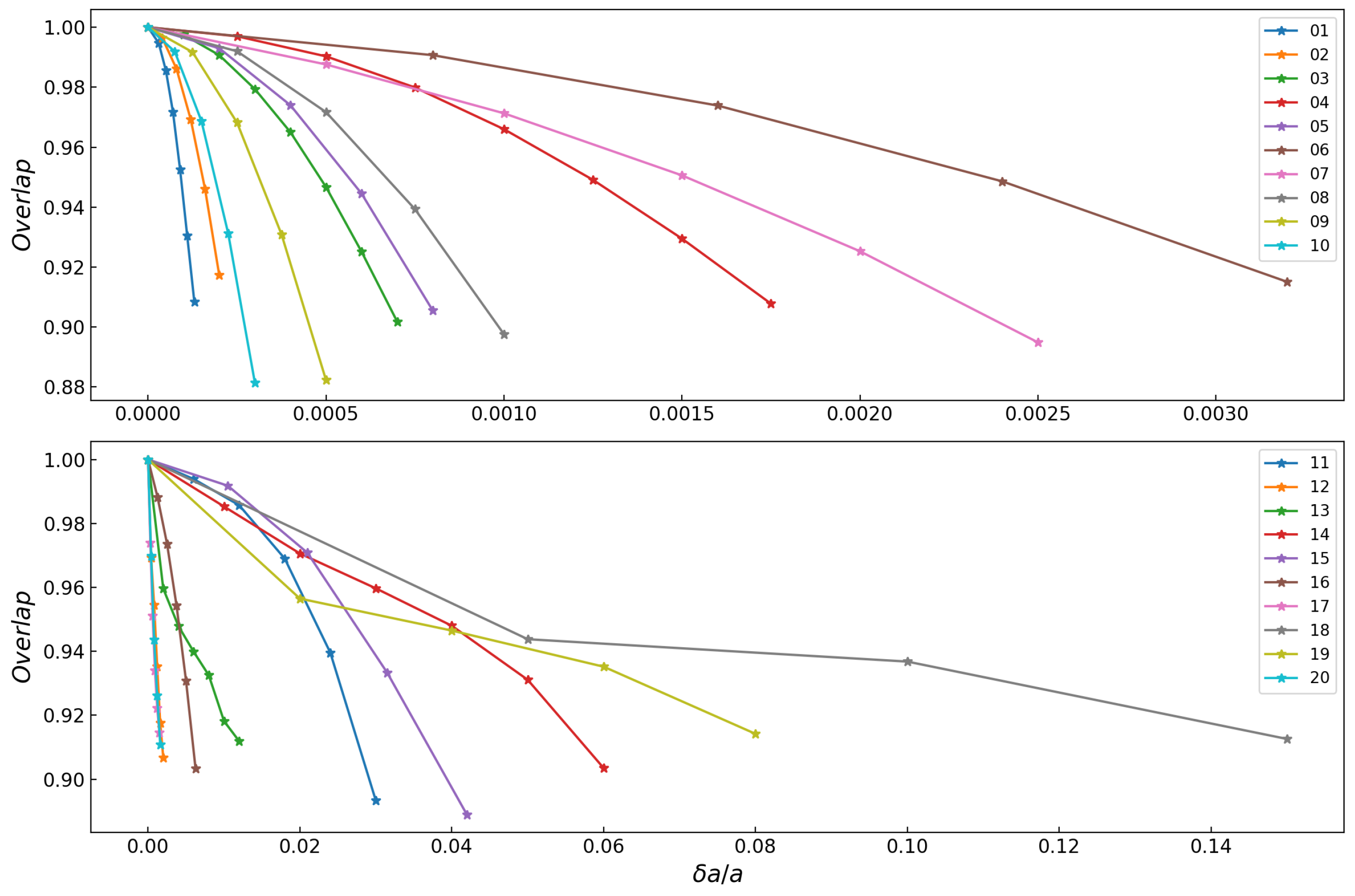
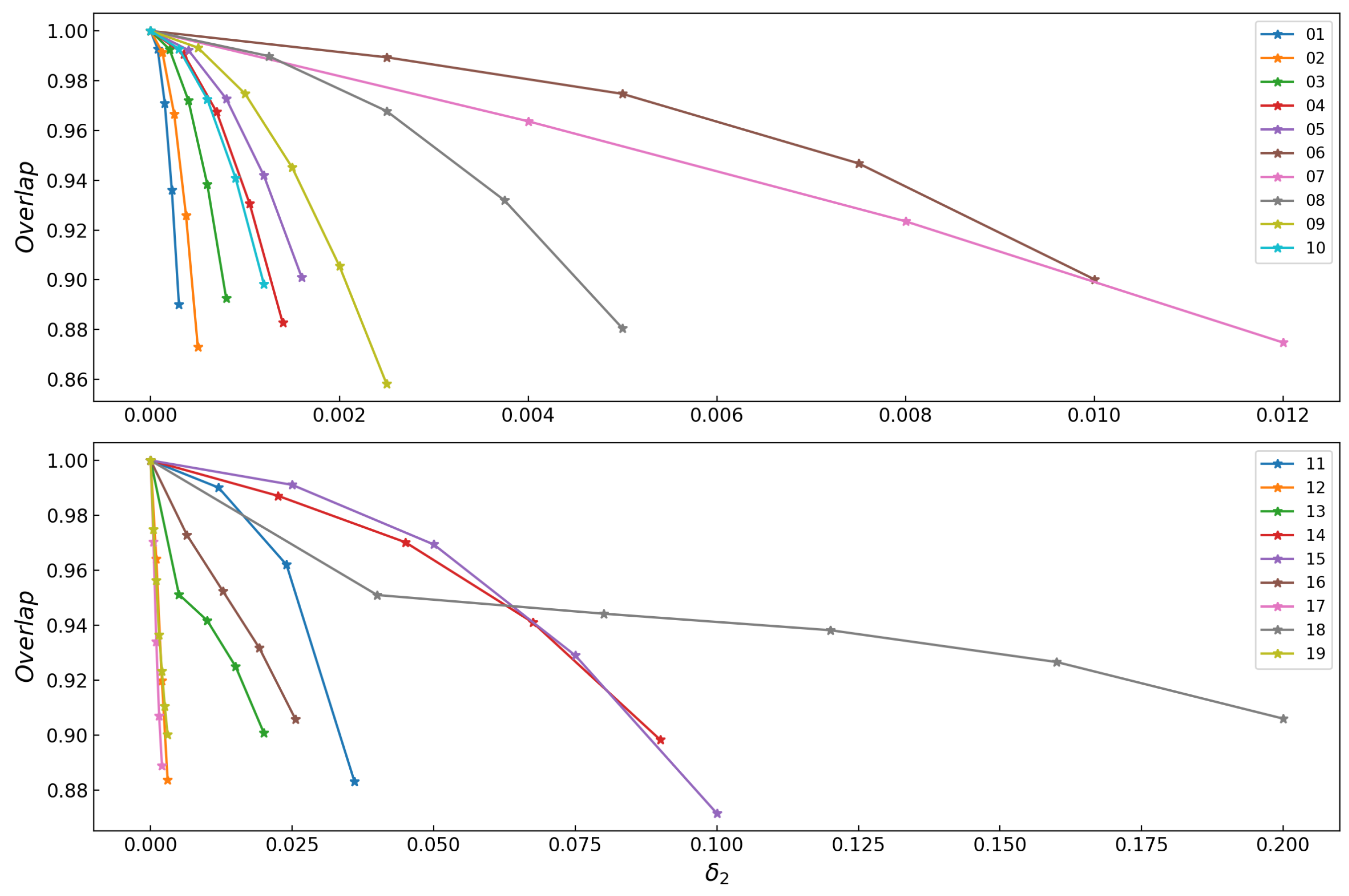
4.1. The Overlaps between Simulated GW Signals of X-MRIs and GW Series with Varying Parameters

Suppose the GW signal and corresponding GW template overlaps are above 0.97 [68]. In that case, we would find neither the deviations from GR nor the unusual parameters of X-MRIs, which is called the confusion problem [68]. The confusion problem can prevent us from obtaining an accurate parameter estimation of the X-MRIs. To make sure there is no confusion in our study, we calculate the overlaps between different gravitational waveforms of twenty X-MRIs with varying parameters λ i ( λ i = a , M , δ 1 , δ 2 , e , p , ι ) . Here, ( a , M ) are the parameters of the Sgr A*, ( δ 1 , δ 2 ) are the deformation parameters of the space-time from the Kerr solution, and ( e , p , ι ) are the parameters of the orbit (eccentricity, semi-latus rectum, inclination).
Because a , M , δ 1 , and δ 2 are the intrinsic parameters of Sgr A* and present the nature of MBH directly, we pay more attention to these four parameters. Figure 1, Figure 2, Figure 3 and Figure 4 display the overlaps between the original waveforms and the waveforms with varying parameters, a , M , δ 1 and δ 2 . As these figures show, the overlap tends to decrease, while the increment of λ increases.
Taking the overlap value 0.97 as a criterion would give the constraints on λ . Specifically, to obtain the constraints on δ λ i by the GWs of X-MRI, we first keep the other parameters fixed and generate several waveforms with varying λ i . Then we calculate the overlaps between the original waveform and the waveforms with varying λ i . Finally, the corresponding value of λ i when the overlap equals 0.97 can be regarded as the limit of λ i . From these figures, we observe the parameter constraint ability for different X-MRI varies.

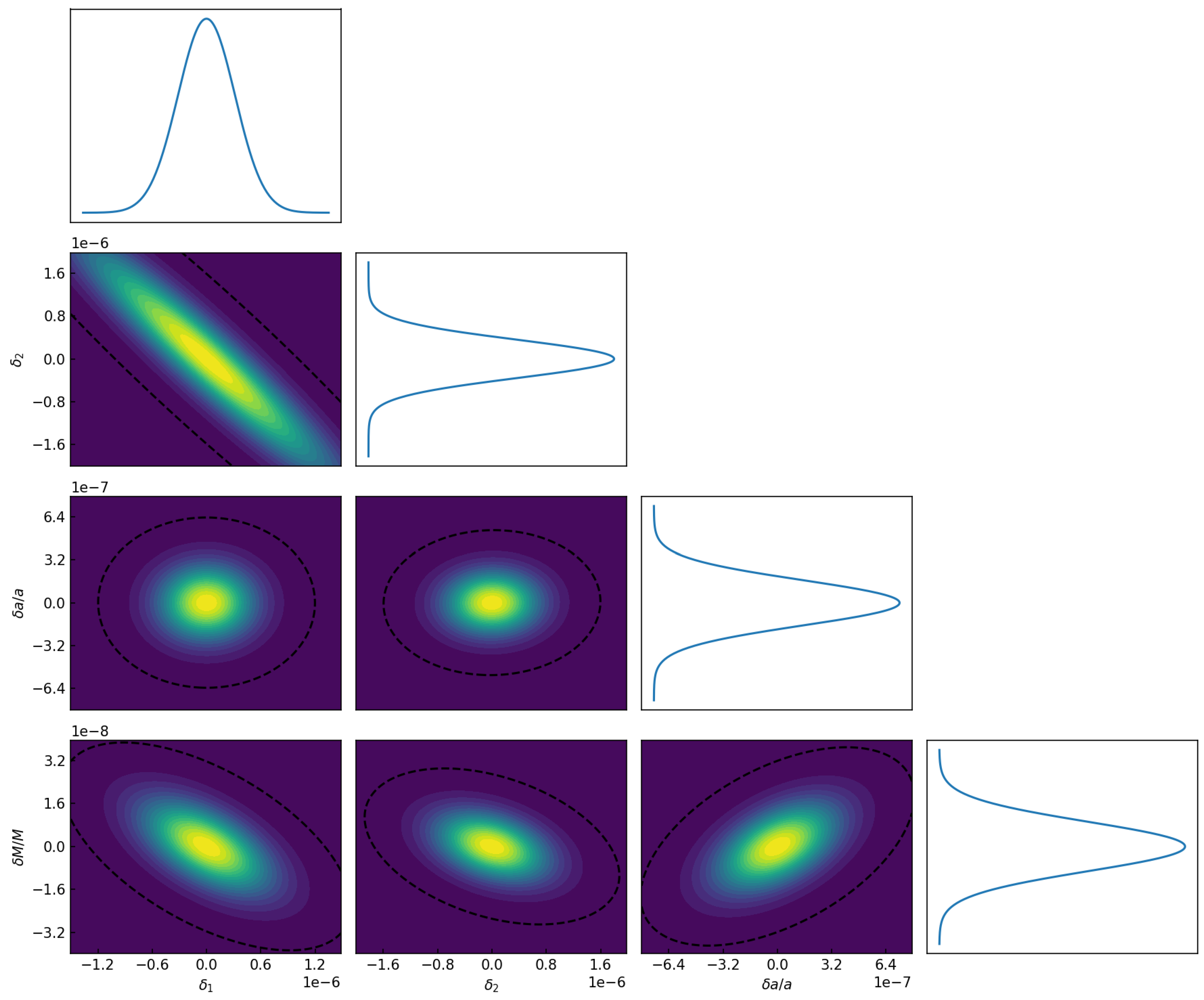
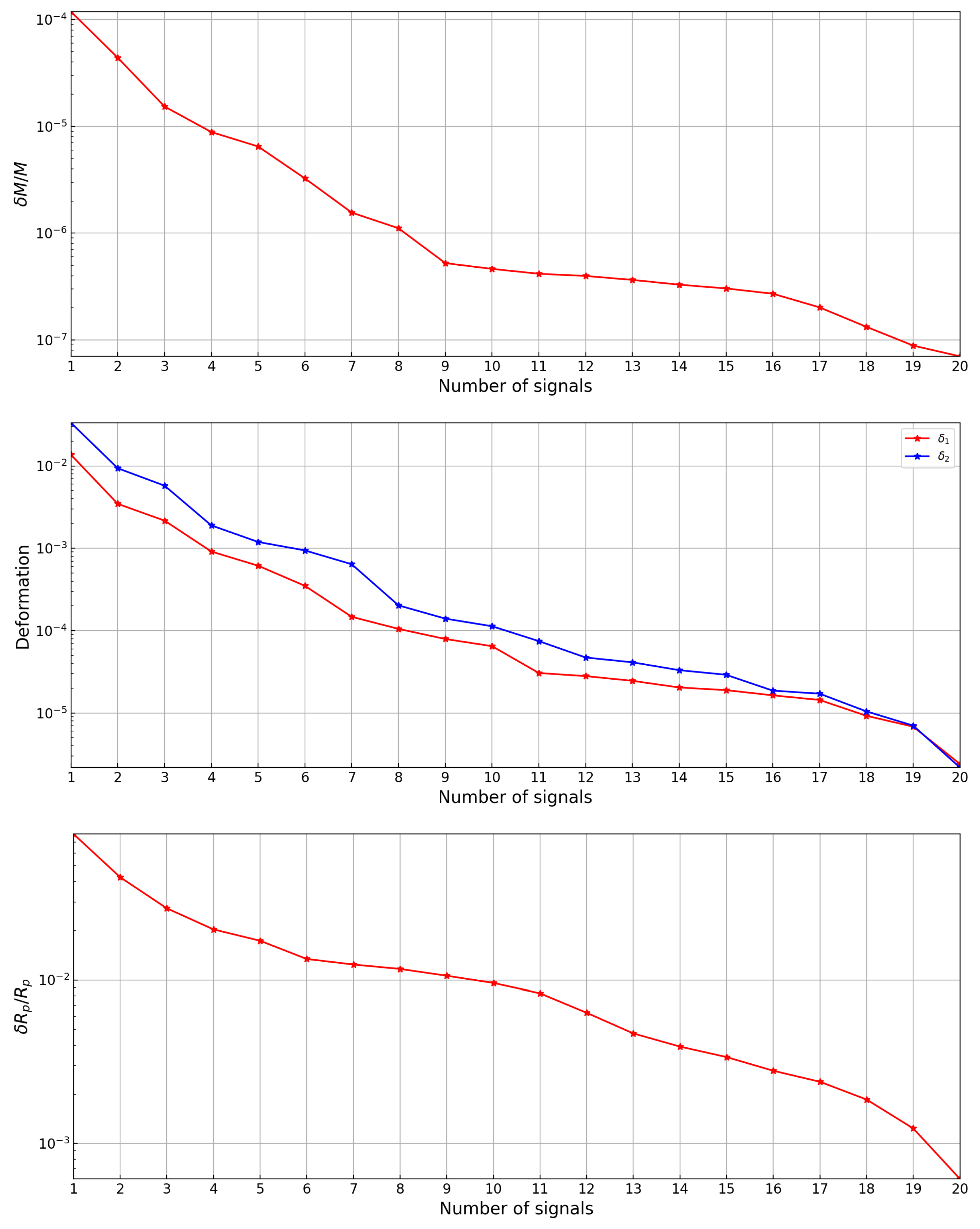
4.2. Evaluate the Accuracy of Parameter Estimation for X-MRIs

The SNRs of the X-MRI GW signals is high enough to apply the Fisher information matrix to estimate the accuracy of parameter estimation. We present the accuracy of parameter estimation for Sgr A* in this part using the Fisher information matrix. To better estimate the distance between Sgr A* and the solar system, we take account of the external parameter R p and constrain it by the gravitational waveforms of the X-MRIs in Table 1.
The Fisher information matrix Γ for a GW signal h parameterized by λ is given by (See Ref. [69] for details)
Γ i , j = < h λ i | h λ j > ,
where λ i = ( a , M , δ 1 , δ 2 , e , p , ι , R p ) is one of the parameters of the X-MRI system. The parameter estimation uncertainty Δ λ due to Gaussian noise has the normal distribution N ( 0 , Γ 1 ) in the case of high SNR, so the root-mean-square uncertainty in the general case can be approximated as
Δ λ i = ( Γ 1 ) i , i .
For the parameter estimation uncertainty Δ λ i , Δ λ j ( i j ) , the corresponding likelihood is [69,70,71].
L ( λ ) e 1 2 Γ i , j Δ λ i Δ λ j .
For an X-MRI with eight parameters, we can obtain a Fisher matrix ( Γ i , j ) 8 × 8 by applying the results of these parameters’ preliminary constraints to Equation (60). Element Γ i , j ( i j ) in the Fisher matrix is the result of the combination of parameter λ i and parameter λ j . With the Fisher matrix, the absolute uncertainty Δ λ i of any parameter λ i can be estimated by calculating Equation (61). Here, we focus on the estimations of Sgr A*’s parameters ( a , M , δ 1 , δ 2 , R p ) .
By using the Fisher matrix, the parameter estimation accuracy of ( a , M , δ 1 , δ 2 , R p ) for the twenty X-MRI signals is shown in Table 1. Different X-MRI systems have different abilities to estimate the uncertainty accuracy of the same parameter. For the spin of Sgr A*, the relative uncertainty Δ a / a estimated by X-MRI 01, X-MRI 02, X-MRI 03, and X-MRI 10 reaches a very high precision, ∼ 10 6 , while Δ a / a estimated by X-MRI 15 is only ∼ 10 2 . For the mass of Sgr A*, its relative uncertainty Δ M / M estimated by X-MRI 01, X-MRI 02, X-MRI 12, and X-MRI 20 reach ∼ 10 7 , and Δ M / M estimated by X-MRI 15 is ∼ 10 4 . For the space-time deformation around Sgr A*, Δ δ 1 and Δ δ 2 estimated by X-MRI 01 reach ∼ 10 6 , while the relative uncertainty of these deformation parameters estimated by X-MRI 15 is only ∼ 10 2 . For the distance R p , its relative uncertainty Δ R p / R p estimated by X-MRI 01 reaches ∼ 10 4 , while the accuracy of Δ R p / R p estimated by X-MRI 06, X-MRI 07, X-MRI 11, and X-MRI 19 is only ∼ 10 2 . From the above analysis, we find that X-MRI 01 has stringent constraints for the five parameters ( a , M , δ 1 , δ 2 , R p ) . Therefore, we take X-MRI 01 as an example to present its likelihoods calculated by Equations (60)–(62). As shown in Figure 5, Figure 6 and Figure 7, it is obvious that the parameter estimation for X-MRI 01 may be affected by any other parameter. Thus, it is reasonable to consider the parameters of one X-MRI signal to estimate any parameter.
We further study the influence of the combination of GW signals on the parameter estimation accuracy. Here, we take parameter α as an example to present the data processing. Firstly, we assume that there are n X-MRI systems at the GC. Then, we calculate the Fisher matrices of all these signals to determine the diagonal element Γ α , α . We sort the value of Γ α , α by the order of size, and the corresponding matrix will be Γ α 1 , Γ α 2 , , Γ α n . Then we add these matrices to obtain the matrix Γ α ,
Γ α = Γ α 1 + Γ α 2 + + Γ α n ,
With Γ α , we obtain the estimation of absolute uncertainty from the equation
Δ α = ( Γ α ) α , α 1 .
We repeat the steps of the estimation for Δ α , and calculate the absolute uncertainty of a , M , δ 1 , δ 2 , R p . Then, we will obtain the relative uncertainty. The results are shown in Figure 8. The accuracy improves as the number of X-MRI increases. As shown in Table 2, with all twenty X-MRI systems, the estimation accuracy for these parameters all reach higher precision. Δ a / a reaches an accuracy of ∼ 10 7 . Δ M / M reaches an accuracy of ∼ 10 8 . Δ δ 1 reaches an accuracy of ∼ 10 6 . Δ δ 2 reaches an accuracy of ∼ 10 6 . Δ R p / R p reaches an accuracy of ∼ 10 4 . The observation number of X-MRI systems does make sense for parameter estimation. Finally, we must emphasize that the parameter estimation results predicted by the Fisher information matrix here only stand for the ideal situation; in the actual parameter estimation practice, because of all kinds of noise, the results would not be that kind of good.

5. Conclusions and Outlook

Sgr A* is the closest MBH to the solar system. It is, therefore, an ideal laboratory to study the properties of black holes and to test alternative theories of gravity. To investigate the structure of Sgr A*, we simulate the GW signals for twenty X-MRI systems using the KRZ metric and the kludge waveform. We then apply the Fisher information matrix method to these GW signals. With a single GW X-MRI event detected, we were able to obtain a relatively accurate estimate of spin a, mass M, and deviation parameters δ 1 and δ 2 . More X-MRI observations would improve the measurement of the above parameters.
In practice, galactic binaries (GBs) and EMRIs are also promising sources of space-borne GW detectors, such as LISA [10]. GBs, comprised primarily of white dwarfs but also neutron stars and stellar-origin black holes, emit continuous and nearly monochromatic GW signals. X-MRIs can be also regarded as monochromatic sources for space-borne detectors, while the signals of X-MRIs can reach high SNRs, making X-MRIs feasible to distinguish from weaker sources such as GBs [16]. On the contrary, EMRIs, which evolve relatively rapidly, are polychromatic sources [16]. Therefore, EMRIs and X-MRIs could be complementary in studying the space-time of MBH.

Author Contributions

Conceptualization, S.-C.Y.; methodology, H.-J.L., Y.-H.Z., C.Z. and S.-C.Y.; software, H.-J.L., Y.-H.Z. and S.-C.Y.; validation, S.-C.Y.; formal analysis, H.-J.L., Y.-H.Z. and S.-C.Y.; investigation, H.-J.L., Y.-H.Z., C.Z. and S.-C.Y.; resources, S.-C.Y.; data curation, H.-J.L., Y.-H.Z. and S.-C.Y.; writing—original draft preparation, H.-J.L.; writing—review and editing, S.-C.Y. and Y.-H.Z.; visualization, H.-J.L.; supervision, S.-C.Y.; project administration, S.-C.Y.; funding acquisition, S.-C.Y. All authors have read and agreed to the published version of the manuscript.

Funding

This work is supported by The National Key R&D Program of China (Grant No. 2021YFC2203002) and NSFC (National Natural Science Foundation of China) Grants No. 11773059 and No. 12173071.

Institutional Review Board Statement

Not applicable.

Informed Consent Statement

Not applicable.

Data Availability Statement

Not applicable.

Acknowledgments

We thank Ahmadjon Abdujabbarov and Imene Belahcene for their valuable advice on this work. This work made use of the High Performance Computing Resource in the Core Facility for Advanced Research Computing at Shanghai Astronomical Observatory.

Conflicts of Interest

The authors declare no conflict of interest.

Abbreviations

The following abbreviations are used in this manuscript:
FFfitting factor
GCGalactic Center
GWgravitational wave
GRgeneral relativity
LIGOLaser Interferometer Gravitation Wave Observatory
LISALaser Interferometer Space Antenna
MBHmassive black hole
SNRsignal-to-noise ratio
X-MRIextremely large mass-ratio inspiral

References

  1. Abbott, B.P.; Abbott, R.; Abbott, T.D.; Abernathy, M.R.; Acernese, F.; Ackley, K.; Adams, C.; Adams, T.; Addesso, P.; Adhikari, R.X.; et al. Observation of gravitational waves from a binary black hole merger. Phys. Rev. Lett. 2016, 116, 061102. [Google Scholar] [CrossRef] [PubMed] [Green Version]
  2. Abbott, B.P.; Abbott, R.; Abbott, T.D.; Acernese, F.; Ackley, K.; Adams, C.; Adams, T.; Addesso, P.; Adhikari, R.X.; Adya, V.B.; et al. GW170817: Observation of gravitational waves from a binary neutron star inspiral. Phys. Rev. Lett. 2017, 119, 161101. [Google Scholar] [CrossRef] [PubMed] [Green Version]
  3. Abbott, B.P.; Abbott, R.; Abbott, T.; Abraham, S.; Acernese, F.; Ackley, K.; Adams, C.; Adhikari, R.X.; Adya, V.B.; Affeldt, C.; et al. GWTC-1: A gravitational-wave transient catalog of compact binary mergers observed by LIGO and Virgo during the first and second observing runs. Phys. Rev. X 2019, 9, 031040. [Google Scholar] [CrossRef] [Green Version]
  4. Abbott, R.; Abbott, T.D.; Abraham, S.; Acernese, F.; Ackley, K.; Adams, A.; Adams, C.; Adhikari, R.X.; Adya, V.B.; Affeldt, C.; et al. GWTC-2: Compact binary coalescences observed by LIGO and Virgo during the first half of the third observing run. Phys. Rev. X 2021, 11, 021053. [Google Scholar]
  5. Abbott, R.; Abbott, T.D.; Acernese, F.; Ackley, K.; Adams, C.; Adhikari, N.; Adhikari, R.X.; Adya, V.B.; Affeldt, C.; Agarwal, D.; et al. GWTC-3: Compact Binary Coalescences Observed by LIGO and Virgo during the Second Part of the Third Observing Run. arXiv 2021, arXiv:2111.03606. [Google Scholar]
  6. Aasi, J.; Abbott, B.P.; Abbott, R.; Abbott, T.; Abernathy, M.R.; Ackley, K.; Adams, C.; Adams, T.; Addesso, P.; Adhikari, R.X.; et al. Advanced LIGO. Class. Quantum Gravity 2015, 32, 074001. [Google Scholar]
  7. Acernese, F.A.; Agathos, M.; Agatsuma, K.; Aisa, D.; Allemandou, N.; Allocca, A.; Amarni, J.; Astone, P.; Balestri, G.; Ballardin, G.; et al. Advanced Virgo: A second-generation interferometric gravitational wave detector. Class. Quantum Gravity 2014, 32, 024001. [Google Scholar] [CrossRef] [Green Version]
  8. The KAGRA Collaboration. KAGRA: 2.5 generation interferometric gravitational wave detector. Nat. Astron. 2019, 3, 35–40. [Google Scholar] [CrossRef] [Green Version]
  9. Amaro-Seoane, P.; Gair, J.R.; Freitag, M.; Miller, M.C.; Mandel, I.; Cutler, C.J.; Babak, S. Intermediate and extreme mass-ratio inspirals—Astrophysics, science applications and detection using LISA. Class. Quantum Gravity 2007, 24, R113. [Google Scholar] [CrossRef]
  10. Amaro-Seoane, P.; Audley, H.; Babak, S.; Baker, J.; Barausse, E.; Bender, P.; Berti, E.; Binetruy, P.; Born, M.; Bortoluzzi, D.; et al. Laser Interferometer Space Antenna. arXiv 2017, arXiv:1702.00786. [Google Scholar]
  11. Hu, W.R.; Wu, Y.L. The Taiji Program in Space for gravitational wave physics and the nature of gravity. Natl. Sci. Rev. 2017, 4, 685. [Google Scholar] [CrossRef]
  12. Luo, J.; Chen, L.S.; Duan, H.Z.; Gong, Y.G.; Hu, S.; Ji, J.; Liu, Q.; Mei, J.; Milyukov, V.; Sazhin, M.; et al. TianQin: A space-borne gravitational wave detector. Class. Quantum Gravity 2016, 33, 035010. [Google Scholar] [CrossRef] [Green Version]
  13. Gair, J.R.; Tang, C.; Volonteri, M. LISA extreme-mass-ratio inspiral events as probes of the black hole mass function. Phys. Rev. D 2010, 81, 104014. [Google Scholar] [CrossRef] [Green Version]
  14. Chua, A.J.; Moore, C.J.; Gair, J.R. Augmented kludge waveforms for detecting extreme-mass-ratio inspirals. Phys. Rev. D 2017, 96, 044005. [Google Scholar] [CrossRef]
  15. Gourgoulhon, E.; Le Tiec, A.; Vincent, F.H.; Warburton, N. Gravitational waves from bodies orbiting the Galactic Center black hole and their detectability by LISA. Astron. Astrophys. 2019, 627, A92. [Google Scholar] [CrossRef] [Green Version]
  16. Amaro-Seoane, P. Extremely large mass-ratio inspirals. Phys. Rev. D 2019, 99, 123025. [Google Scholar] [CrossRef] [Green Version]
  17. Burrows, A.; Liebert, J. The science of brown dwarfs. Rev. Mod. Phys. 1993, 65, 301. [Google Scholar] [CrossRef]
  18. Freitag, M. Gravitational waves from stars orbiting the Sagittarius A* black hole. ApJ 2002, 583, L21. [Google Scholar] [CrossRef]
  19. Eckart, A.; Genzel, R. Observations of stellar proper motions near the Galactic Centre. Nature 1996, 383, 415–417. [Google Scholar] [CrossRef]
  20. Ghez, A.M.; Klein, B.; Morris, M.; Becklin, E. High proper-motion stars in the vicinity of Sagittarius A*: Evidence for a supermassive black hole at the center of our galaxy. ApJ 1998, 509, 678. [Google Scholar] [CrossRef] [Green Version]
  21. Ghez, A.M.; Salim, S.; Weinberg, N.; Lu, J.; Do, T.; Dunn, J.; Matthews, K.; Morris, M.; Yelda, S.; Becklin, E.; et al. Measuring distance and properties of the Milky Way’s central supermassive black hole with stellar orbits. ApJ 2008, 689, 1044. [Google Scholar] [CrossRef] [Green Version]
  22. Genzel, R.; Eisenhauer, F.; Gillessen, S. The Galactic Center massive black hole and nuclear star cluster. Rev. Mod. Phys. 2010, 82, 3121. [Google Scholar] [CrossRef]
  23. Afrin, M.; Kumar, R.; Ghosh, S.G. Parameter estimation of hairy Kerr black holes from its shadow and constraints from M87. MNRAS 2021, 504, 5927–5940. [Google Scholar] [CrossRef]
  24. Konoplya, R.; Rezzolla, L.; Zhidenko, A. General parametrization of axisymmetric black holes in metric theories of gravity. Phys. Rev. D 2016, 93, 064015. [Google Scholar] [CrossRef]
  25. Abbott, R.; Abe, H.; Acernese, F.; Ackley, K.; Adhikari, N.; Adhikari, R.X.; Adkins, V.K.; Adya, V.B.; Affeldt, C.; Agarwal, D.; et al. Tests of General Relativity with GWTC-3. arXiv 2021, arXiv:gr-qc/2112.06861. [Google Scholar]
  26. Hu, S.; Deng, C.; Li, D.; Wu, X.; Liang, E. Observational signatures of Schwarzschild-MOG black holes in scalar-tensor-vector gravity: Shadows and rings with different accretions. Eur. Phys. J. C 2022, 82, 1–17. [Google Scholar]
  27. Cao, W.; Liu, W.; Wu, X. Integrability of Kerr-Newman spacetime with cloud strings, quintessence and electromagnetic field. Phys. Rev. D 2022, 105, 124039. [Google Scholar] [CrossRef]
  28. Zhang, H.; Zhou, N.; Liu, W.; Wu, X. Equivalence between two charged black holes in dynamics of orbits outside the event horizons. Gen. Relat. Gravity 2022, 54, 1–22. [Google Scholar] [CrossRef]
  29. Yang, D.; Cao, W.; Zhou, N.; Zhang, H.; Liu, W.; Wu, X. Chaos in a Magnetized Modified Gravity Schwarzschild Spacetime. Universe 2022, 8, 320. [Google Scholar] [CrossRef]
  30. Zhang, H.; Zhou, N.; Liu, W.; Wu, X. Charged particle motions near non-Schwarzschild black holes with external magnetic fields in modified theories of gravity. Universe 2021, 7, 488. [Google Scholar] [CrossRef]
  31. Yi, M.; Wu, X. Dynamics of charged particles around a magnetically deformed Schwarzschild black hole. Phys. Scr. 2020, 95, 085008. [Google Scholar] [CrossRef]
  32. Johannsen, T.; Psaltis, D. Metric for rapidly spinning black holes suitable for strong-field tests of the no-hair theorem. Phys. Rev. D 2011, 83, 124015. [Google Scholar] [CrossRef] [Green Version]
  33. Ni, Y.; Jiang, J.; Bambi, C. Testing the Kerr metric with the iron line and the KRZ parametrization. J. Cosmol. Astropart. Phys. 2016, 2016, 014. [Google Scholar] [CrossRef] [Green Version]
  34. Drake, S.P.; Szekeres, P. Uniqueness of the Newman–Janis algorithm in generating the Kerr–Newman metric. Gen. Relativ. Gravity 2000, 32, 445–457. [Google Scholar] [CrossRef] [Green Version]
  35. Jiang, J.; Bambi, C.; Steiner, J.F. Using iron line reverberation and spectroscopy to distinguish Kerr and non-Kerr black holes. JCAP 2015, 2015, 025. [Google Scholar] [CrossRef] [Green Version]
  36. Horne, J.H.; Horowitz, G.T. Rotating dilaton black holes. Phys. Rev. D 1992, 46, 1340. [Google Scholar] [CrossRef]
  37. Cardoso, V.; Pani, P.; Rico, J. On generic parametrizations of spinning black-hole geometries. Phys. Rev. D 2014, 89, 064007. [Google Scholar] [CrossRef] [Green Version]
  38. Younsi, Z.; Zhidenko, A.; Rezzolla, L.; Konoplya, R.; Mizuno, Y. New method for shadow calculations: Application to parametrized axisymmetric black holes. Phys. Rev. D 2016, 94, 084025. [Google Scholar] [CrossRef] [Green Version]
  39. Zhou, N.; Zhang, H.; Liu, W.; Wu, X. A Note on the Construction of Explicit Symplectic Integrators for Schwarzschild Spacetimes. ApJ 2022, 927, 160. [Google Scholar] [CrossRef]
  40. Wang, Y.; Sun, W.; Liu, F.; Wu, X. Construction of Explicit Symplectic Integrators in General Relativity. I. Schwarzschild Black Holes. ApJ 2021, 907, 66. [Google Scholar] [CrossRef]
  41. Wang, Y.; Sun, W.; Liu, F.; Wu, X. Construction of Explicit Symplectic Integrators in General Relativity. II. Reissner–Nordström Black Holes. ApJ 2021, 909, 22. [Google Scholar] [CrossRef]
  42. Wang, Y.; Sun, W.; Liu, F.; Wu, X. Construction of Explicit Symplectic Integrators in General Relativity. III. Reissner–Nordström-(anti)-de Sitter Black Holes. ApJ S 2021, 254, 8. [Google Scholar] [CrossRef]
  43. Wu, X.; Wang, Y.; Sun, W.; Liu, F. Construction of explicit symplectic integrators in general relativity. IV. Kerr black holes. ApJ 2021, 914, 63. [Google Scholar] [CrossRef]
  44. Sun, W.; Wang, Y.; Liu, F.; Wu, X. Applying explicit symplectic integrator to study chaos of charged particles around magnetized Kerr black hole. Eur. Phys. J. C 2021, 81, 1–10. [Google Scholar] [CrossRef]
  45. Xin, S.; Han, W.B.; Yang, S.C. Gravitational waves from extreme-mass-ratio inspirals using general parametrized metrics. Phys. Rev. D 2019, 100, 084055. [Google Scholar] [CrossRef] [Green Version]
  46. Hughes, S.A. Evolution of circular, nonequatorial orbits of Kerr black holes due to gravitational-wave emission. II. Inspiral trajectories and gravitational waveforms. Phys. Rev. D 2001, 64, 064004. [Google Scholar] [CrossRef]
  47. Barack, L.; Cutler, C. LISA capture sources: Approximate waveforms, signal-to-noise ratios, and parameter estimation accuracy. Phys. Rev. D 2004, 69, 082005. [Google Scholar] [CrossRef] [Green Version]
  48. Drasco, S.; Hughes, S.A. Gravitational wave snapshots of generic extreme mass ratio inspirals. Phys. Rev. D 2006, 73, 024027. [Google Scholar] [CrossRef] [Green Version]
  49. Babak, S.; Fang, H.; Gair, J.R.; Glampedakis, K.; Hughes, S.A. “Kludge” gravitational waveforms for a test-body orbiting a Kerr black hole. Phys. Rev. D 2007, 75, 024005. [Google Scholar] [CrossRef] [Green Version]
  50. Chua, A.J.; Gair, J.R. Improved analytic extreme-mass-ratio inspiral model for scoping out eLISA data analysis. Class. Quantum Gravity 2015, 32, 232002. [Google Scholar] [CrossRef]
  51. Rüdiger, R. Conserved quantities of spinning test particles in general relativity. I. Proc. R. Soc. Lond. Math. Phys. Sci. 1981, 375, 185–193. [Google Scholar]
  52. Rüdiger, R. Conserved quantities of spinning test particles in general relativity. II. Proc. R. Soc. Lond. Math. Phys. Sci. 1983, 385, 229–239. [Google Scholar]
  53. Wang, S.C.; Wu, X.; Liu, F.Y. Implementation of the velocity scaling method for elliptic restricted three-body problems. MNRAS 2016, 463, 1352–1362. [Google Scholar] [CrossRef]
  54. Wang, S.; Huang, G.; Wu, X. Simulations of dissipative circular restricted three-body problems using the velocity-scaling correction method. ApJ 2018, 155, 67. [Google Scholar] [CrossRef]
  55. Deng, C.; Wu, X.; Liang, E. The use of Kepler solver in numerical integrations of quasi-Keplerian orbits. MNRAS 2020, 496, 2946–2961. [Google Scholar] [CrossRef]
  56. Li, D.; Wu, X. Modification of logarithmic Hamiltonians and application of explicit symplectic-like integrators. MNRAS 2017, 469, 3031–3041. [Google Scholar] [CrossRef]
  57. Luo, J.; Wu, X.; Huang, G.; Liu, F. Explicit symplectic-like integrators with midpoint permutations for spinning compact binaries. ApJ 2017, 834, 64. [Google Scholar] [CrossRef]
  58. Pan, G.; Wu, X.; Liang, E. Extended phase-space symplectic-like integrators for coherent post-Newtonian Euler-Lagrange equations. Phys. Rev. D 2021, 104, 044055. [Google Scholar] [CrossRef]
  59. Liu, L.; Wu, X.; Huang, G.; Liu, F. Higher order explicit symmetric integrators for inseparable forms of coordinates and momenta. MNRAS 2016, 459, 1968–1976. [Google Scholar] [CrossRef] [Green Version]
  60. Mei, L.; Wu, X.; Liu, F. On preference of Yoshida construction over Forest–Ruth fourth-order symplectic algorithm. Eur. Phys. J. C 2013, 73, 1–8. [Google Scholar] [CrossRef]
  61. Mei, L.; Ju, M.; Wu, X.; Liu, S. Dynamics of spin effects of compact binaries. MNRAS 2013, 435, 2246–2255. [Google Scholar] [CrossRef] [Green Version]
  62. Zhong, S.Y.; Wu, X.; Liu, S.Q.; Deng, X.F. Global symplectic structure-preserving integrators for spinning compact binaries. Phys. Rev. D 2010, 82, 124040. [Google Scholar] [CrossRef]
  63. Finn, L.S. Detection, measurement, and gravitational radiation. Phys. Rev. D 1992, 46, 5236. [Google Scholar] [CrossRef] [PubMed] [Green Version]
  64. Chabrier, G.; Baraffe, I. Theory of low-mass stars and substellar objects. Annu. Rev. Astron. Astrophys. 2000, 38, 337–377. [Google Scholar] [CrossRef] [Green Version]
  65. Shcherbakov, R.V.; Penna, R.F.; McKinney, J.C. Sagittarius A* accretion flow and black hole parameters from general relativistic dynamical and polarized radiative modeling. ApJ 2012, 755, 133. [Google Scholar] [CrossRef]
  66. Eisenhauer, F.; Schödel, R.; Genzel, R.; Ott, T.; Tecza, M.; Abuter, R.; Eckart, A.; Alexander, T. A geometric determination of the distance to the galactic center. ApJ 2003, 597, L121. [Google Scholar] [CrossRef]
  67. Menten, K.M.; Reid, M.J.; Eckart, A.; Genzel, R. The position of Sagittarius A*: Accurate alignment of the radio and infrared reference frames at the Galactic Center. ApJ 1997, 475, L111. [Google Scholar] [CrossRef] [Green Version]
  68. Glampedakis, K.; Babak, S. Mapping spacetimes with LISA: Inspiral of a test body in a ‘quasi-Kerr’field. Class. Quantum Gravity 2006, 23, 4167. [Google Scholar] [CrossRef]
  69. Cutler, C.; Flanagan, E.E. Gravitational waves from merging compact binaries: How accurately can one extract the binary’s parameters from the inspiral waveform? Phys. Rev. D 1994, 49, 2658. [Google Scholar] [CrossRef] [Green Version]
  70. Babak, S.; Gair, J.; Sesana, A.; Barausse, E.; Sopuerta, C.F.; Berry, C.P.; Berti, E.; Amaro-Seoane, P.; Petiteau, A.; Klein, A. Science with the space-based interferometer LISA. V. Extreme mass-ratio inspirals. Phys. Rev. D 2017, 95, 103012. [Google Scholar] [CrossRef] [Green Version]
  71. Han, W.B.; Chen, X. Testing general relativity using binary extreme-mass-ratio inspirals. MNRAS 2019, 485, L29–L33. [Google Scholar] [CrossRef]
Figure 1. Overlaps between the original waveforms and the waveforms changed with spin a. The other parameters (M, δ 1 , δ 2 , e, p, ι ) of systems listed in Table 1 remain unchanged. The top plane represents a-overlap curves from the top 10 systems (X-MRI 01 to X-MRI 10). The bottom plane represents a-overlap curves from the last 10 systems (X-MRI 11 to X-MRI 20).
Symmetry 14 02558 g001
Figure 2. Overlaps between the original waveforms and the waveforms changed with mass M. The other parameters (a, δ 1 , δ 2 , e, p, ι ) of systems listed in Table 1 remain unchanged. The top plane represents M-overlap curves from the top 10 systems (X-MRI 01 to X-MRI 10). The bottom plane represents M-overlap curves from the last 10 systems (X-MRI 11 to X-MRI 20).
Symmetry 14 02558 g002
Figure 3. Overlaps between the original waveforms and the waveforms changed with deformation parameter δ 1 . The other parameters (M, a, δ 2 , e, p, ι ) of systems listed in Table 1 remain unchanged. The top plane represents δ 1 -overlap curves from the top 10 systems (X-MRI 01 to X-MRI 10). The bottom plane represents δ 1 -overlap curves from the last 10 systems (X-MRI 11 to X-MRI 20).
Symmetry 14 02558 g003
Figure 4. Overlaps between the original waveforms and the waveforms changed with deformation parameter δ 2 . The other parameters (M, a, δ 1 , e, p, ι ) of systems listed in Table 1 remain unchanged. The top plane represents δ 2 -overlap curves from the top 10 systems (X-MRI 01 to X-MRI 10). The bottom plane represents δ 2 -overlap curves from the last 10 systems (X-MRI 11 to X-MRI 20).
Symmetry 14 02558 g004
Figure 5. Likelihoods of ( δ 1 , δ M / M ) , ( δ 1 , δ a / a ) , ( δ 1 , δ 2 ) , ( δ 2 , δ M / M ) , ( δ 2 , δ a / a ) , and ( δ a / a , δ M / M ) derived from the Fisher matrix of X-MRI 01. The black dashed eclipses show the 3 σ confidence level. The upper and the four right-hand panels show the marginalized probability distribution for δ 1 , δ 2 , δ a / a and δ M / M , respectively.
Symmetry 14 02558 g005
Figure 6. Likelihoods of ( δ a / a , δ e / e ) , ( δ a / a , δ p / p ) , ( δ a / a , δ ι / ι ) , ( δ a / a , δ R p / R p ) , ( δ M / M , δ e / e ) , ( δ M / M , δ p / p ) , ( δ M / M , δ ι / ι ) , ( δ M / M , δ R p / R p ) , ( δ 1 , δ e / e ) , ( δ 1 , δ p / p ) , ( δ 1 , δ ι / ι ) , ( δ 1 , δ R p / R p ) , ( δ 2 , δ e / e ) , ( δ 2 , δ p / p ) , ( δ 2 , δ ι / ι ) , and ( δ 2 , δ R p / R p ) derived from the Fisher matrix of X-MRI 01. The black dashed eclipses show the 3 σ confidence level.
Symmetry 14 02558 g006
Figure 7. Likelihoods of ( δ e / e , δ R p / R p ) , ( δ e / e , δ ι / ι ) , ( δ e / e , δ p / p ) , ( δ p / p , δ R p / R p ) , ( δ p / p , δ ι / ι ) , ( δ ι / ι , δ R p / R p ) derived from the Fisher matrix of X-MRI 01. The black dashed eclipses show the 3 σ confidence level. The upper and the four right-hand panels show the marginalized probability distribution for δ e / e , δ p / p , δ ι / ι , and δ R p / R p , respectively.
Symmetry 14 02558 g007
Figure 8. The relation between the parameter estimation accuracy and the X-MRI signal number. The parameter in the first plane is δ a / a , in the second plane is δ M / M , in the third plane are δ 1 (red) and δ 2 (blue), and in the fourth plane is δ R p / R p .
Symmetry 14 02558 g008aSymmetry 14 02558 g008b
Table 1. Parameter setting and parameter estimation accuracy for the 20 X-MRIs at the GC.
Signalep ι M Object SNR Δ a / a Δ M / M Δ δ 1 Δ δ 2 Δ R p / R p
01 0.617 10.600 5 π / 6 2.80 × 10 2 1584.363 2.85 × 10 6 4.18 × 10 7 3.63 × 10 6 3.28 × 10 6 7.18 × 10 4
02 0.520 12.000 π / 6 2.00 × 10 2 636.988 2.10 × 10 6 9.53 × 10 7 1.48 × 10 5 1.48 × 10 5 1.78 × 10 3
03 0.300 14.400 π / 6 2.00 × 10 2 224.915 9.39 × 10 6 4.04 × 10 6 3.92 × 10 5 4.95 × 10 5 5.03 × 10 3
04 0.200 16.800 π / 7 2.72 × 10 2 144.765 4.60 × 10 5 4.54 × 10 6 7.31 × 10 5 1.04 × 10 4 7.37 × 10 3
05 0.400 16.800 π / 7 2.72 × 10 2 201.217 1.33 × 10 5 2.91 × 10 6 6.17 × 10 5 8.26 × 10 5 5.29 × 10 3
06 0.514 27.243 π / 12 1.80 × 10 2 30.518 2.47 × 10 4 1.96 × 10 5 8.48 × 10 4 1.39 × 10 3 3.58 × 10 2
07 0.500 24.750 π / 4 3.60 × 10 2 59.061 7.79 × 10 5 3.33 × 10 6 1.70 × 10 4 3.44 × 10 4 1.68 × 10 2
08 0.600 19.200 π / 5 2.80 × 10 2 148.460 1.92 × 10 5 1.91 × 10 6 1.21 × 10 4 1.92 × 10 4 6.92 × 10 3
09 0.700 15.300 π / 6 1.00 × 10 2 140.487 1.15 × 10 5 4.43 × 10 6 1.54 × 10 4 1.80 × 10 4 7.73 × 10 3
10 0.800 12.600 π / 8 1.20 × 10 2 355.391 4.80 × 10 6 3.42 × 10 6 6.45 × 10 5 6.18 × 10 5 3.27 × 10 3
11 0.100 39.600 π / 6 7.00 × 10 2 32.112 5.38 × 10 3 6.25 × 10 5 3.66 × 10 3 9.96 × 10 3 5.57 × 10 2
12 0.253 35.093 π / 3 7.84 × 10 2 39.303 7.72 × 10 5 2.36 × 10 7 4.13 × 10 5 1.41 × 10 4 2.63 × 10 2
13 0.206 30.159 π / 4 7.60 × 10 2 45.575 1.38 × 10 4 1.94 × 10 6 1.56 × 10 4 3.69 × 10 4 2.25 × 10 2
14 0.368 41.053 π / 7 8.00 × 10 2 47.910 1.49 × 10 3 1.23 × 10 5 3.00 × 10 3 8.19 × 10 3 3.61 × 10 2
15 0.295 47.924 π / 9 6.00 × 10 2 24.535 1.03 × 10 2 1.18 × 10 4 1.37 × 10 2 3.34 × 10 2 7.85 × 10 2
16 0.425 32.775 π / 11 3.00 × 10 2 19.701 6.08 × 10 4 2.15 × 10 5 1.04 × 10 3 1.99 × 10 3 5.27 × 10 2
17 0.300 27.300 π / 3 3.20 × 10 2 27.179 9.05 × 10 5 1.01 × 10 6 7.17 × 10 5 2.40 × 10 4 3.78 × 10 2
18 0.133 44.200 2 π / 3 6.80 × 10 2 29.731 9.80 × 10 4 2.19 × 10 6 4.83 × 10 4 2.21 × 10 3 3.43 × 10 2
19 0.137 50.039 π / 3 7.20 × 10 2 24.736 1.04 × 10 3 2.53 × 10 6 7.36 × 10 5 2.42 × 10 3 4.07 × 10 2
20 0.477 25.108 3 π / 5 8.00 × 10 2 101.345 4.48 × 10 5 2.05 × 10 7 1.16 × 10 5 3.58 × 10 5 9.75 × 10 3
Table 2. Results of parameter estimation accuracy of all 20 X-MRI systems.
Δ a / a Δ M / M Δ δ 1 Δ δ 2 Δ R p / R p
5.38 × 10 7 7.02 × 10 8 2.40 × 10 6 2.18 × 10 6 6.05 × 10 4
Publisher’s Note: MDPI stays neutral with regard to jurisdictional claims in published maps and institutional affiliations.

