
An Innovative Hybrid Multi-Criteria Decision-Making Approach under Picture Fuzzy Information


Abstract
:1. Introduction
- Existing decision-making structures, including PFSSs, are unable to deal with the bipolarity of decision attributes efficiently.
- Models such as BSSs and fuzzy BSSs which are capable of depicting the bipolarity of attributes fail to handle uncertainties effectively since they fail to consider positive, negative, and neutral degrees of opinion.
- Problems such as selection of a fashion designer specific to the company’s needs are complicated MCDM problems requiring a strong decision-making algorithm.
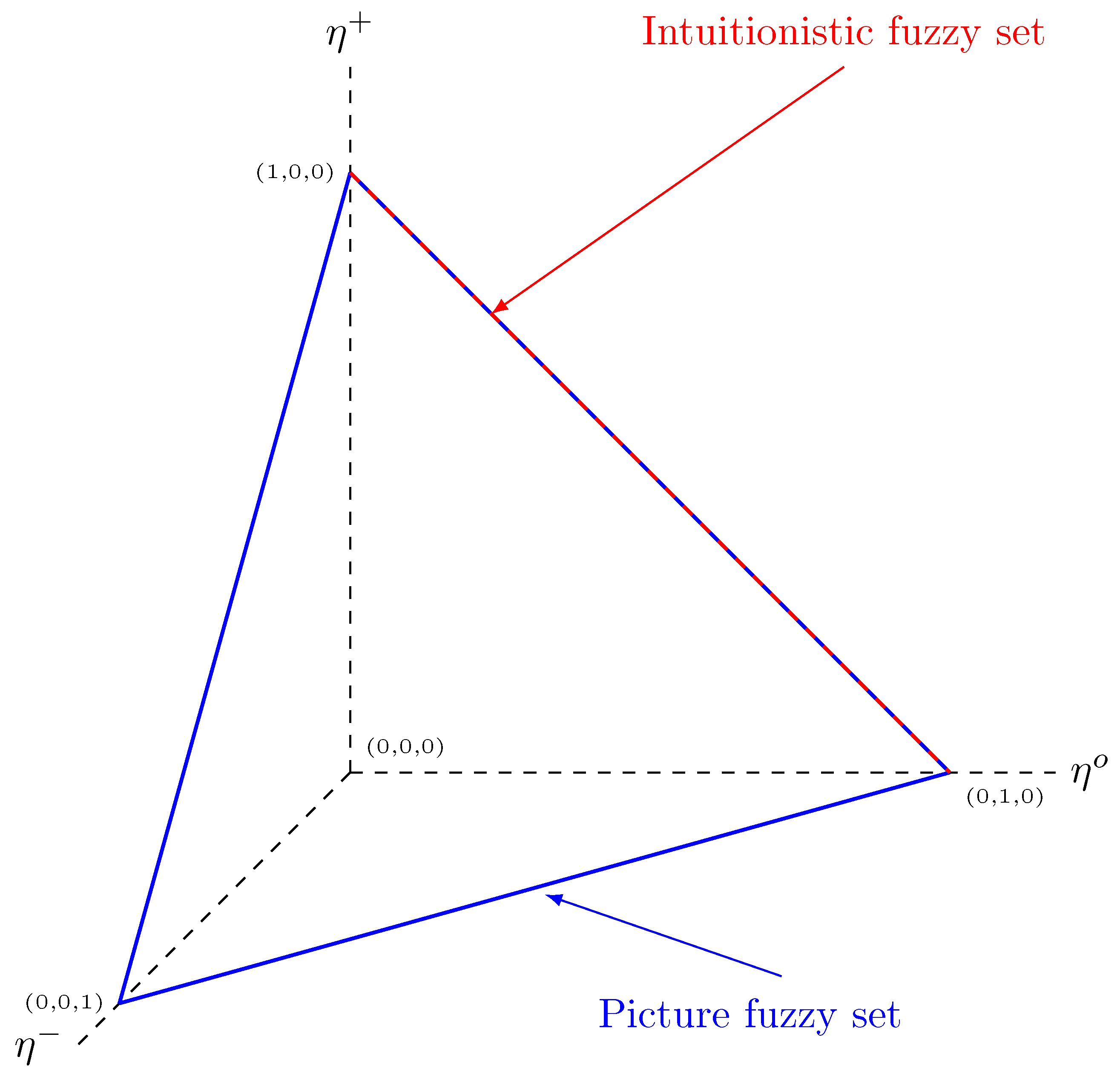
- A model called picture fuzzy bipolar soft set (or PFBSS), a natural hybrid extension of PFS and BSS, is proposed.
- Some novel properties and two fundamental operations of PFBSSs are presented and illustrated via corresponding numerical examples.
- Important results including the commutative, associative, and distributive properties are presented. Furthermore, De Morgan’s Laws for the proposed properties and operations are shown.
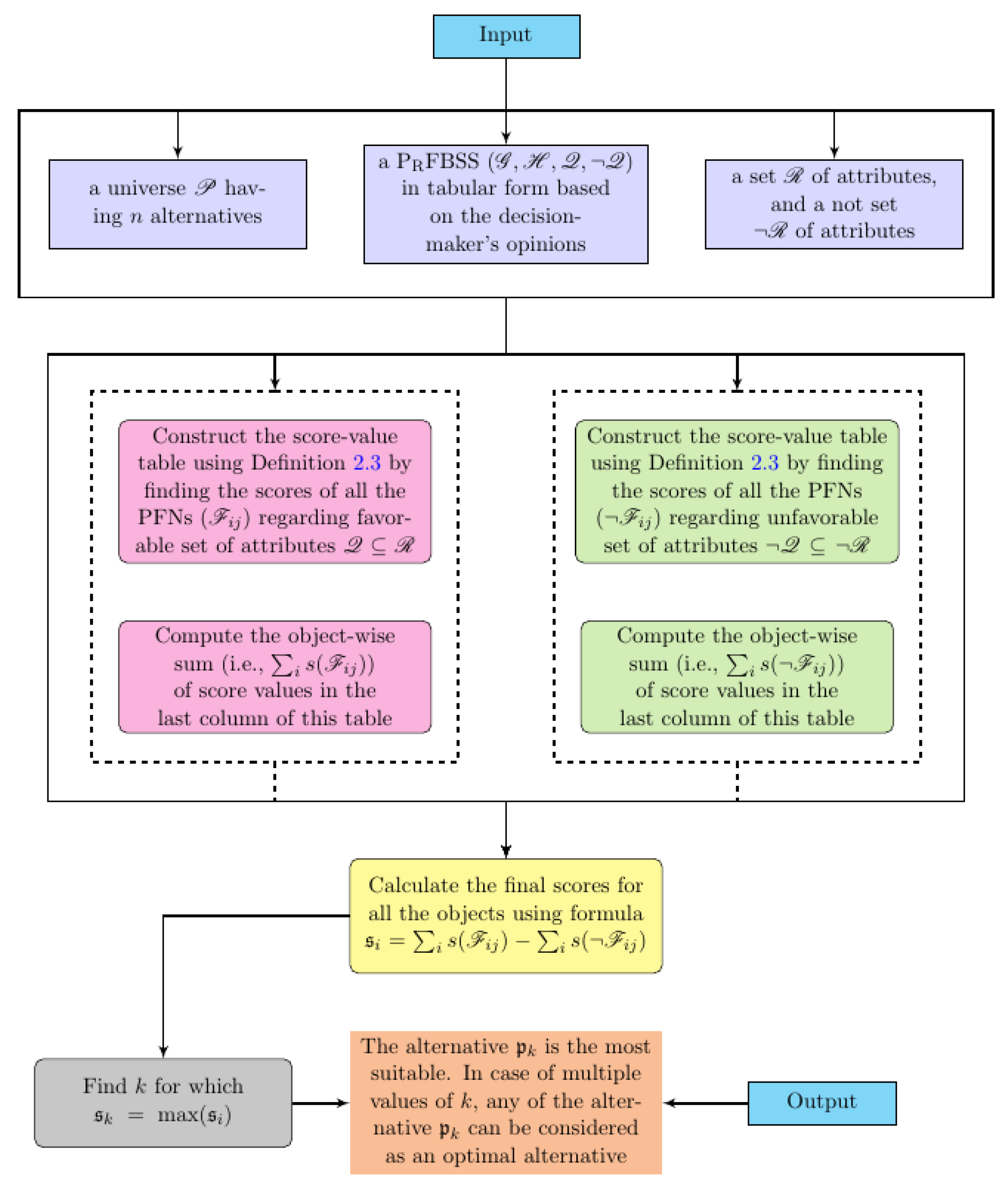
- A PFBSS-based algorithm using score functions for picture fuzzy numbers is presented to deal with MCDM problems considering the decision attributes in symmetry.
- An MCDM application of PFBSSs, i.e., the selection of a fashion designer for a studio, is presented and solved using the newly proposed algorithm based on PFBSSs.
- Finally, a detailed comparative analysis concerning both qualitative and quantitative perspectives of the proposed model with certain existing models is provided.
Organization of Paper
2. Preliminaries
- (i)
- <; or
- (ii)
- = and <.
3. Picture Fuzzy Bipolar Soft Sets
- 1.
- ;
- 2.
- , that is, ≤, ≤ and ≥∈;
- 3.
- , that is, ≤, ≤ and ≥ and ∈.
- 1.
- 2.
- 3.
- 4.
- 5.
- 6.
- Suppose thatThen, by Definition 10, we have:Similarly, we have:Such that, and ,Hence,
- Suppose thatThen, by Definition 11, we have:Similarly, we have:Such that, and ,Hence,
- 1.
- 2.
- From Definitions 8 and 10,where we haveSimilarly, we have:Such that, and ,Hence,
- From Definitions 8 and 11,where we have:Similarly, we have:Such that, and ,Hence,
- 1.
- 2.
- 3.
- 4.
- From Definition 12:Such that :Similarly,This implies thatHence,
- From Definition 13:Such that ,and ,This implies thatHence,
- 1.
- 2.
- 3.
- 4.
- From Definition 14:Such that ,Similarly,This implies thatHence,
- From Definition 15:Such that ,and ,This implies thatHence,
- 1.
- 2.
- 3.
- 4.
- 1.
- is the minimal PFBSS over containing both and .
- 2.
- is the maximal PFBSS over that is contained in both and .
- 1.
- 2.
- 3.
- 4.
- By Definitions 8 and 12, we obtainwhere:Hence, .
- By Definitions 8 and 13, we obtain:where, for allSimilarly, for allHence, .
4. Application to MCDM
| Algorithm 1: Selection of best alternative under PFBSS environment. |
|
Application: Selection of Best Graphic Designer for a Studio
5. Comparison
5.1. Advantages
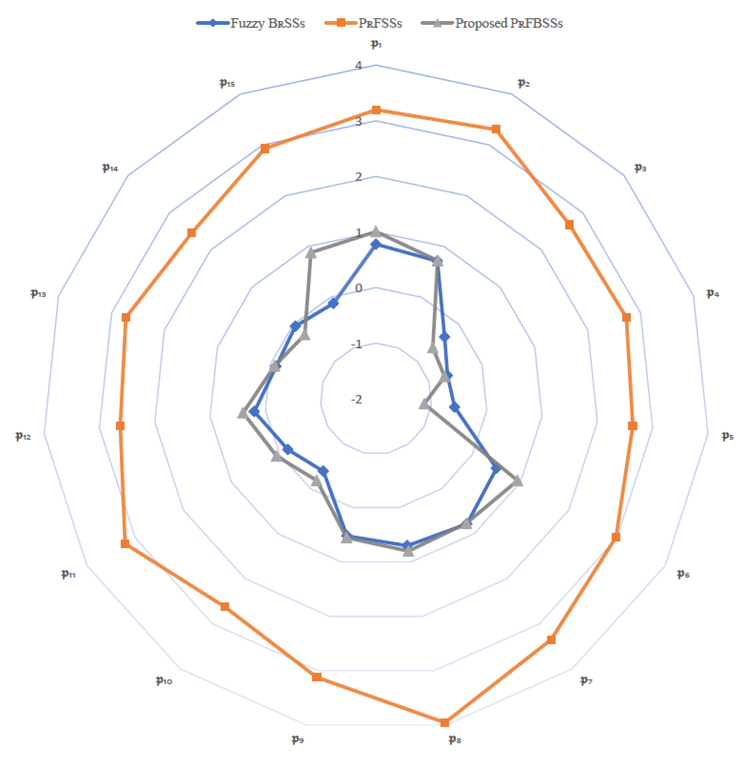
5.2. Comparison
5.3. Limitations
6. Conclusions and Future Directions
- Rough picture fuzzy bipolar soft sets;
- Picture fuzzy bipolar soft expert sets;
- Picture fuzzy bipolar soft aggregation operators;
- q-Rung picture fuzzy bipolar soft sets;
- Interval-valued picture fuzzy bipolar soft sets;
- Rough picture fuzzy bipolar soft expert sets.
Author Contributions
Funding
Institutional Review Board Statement
Informed Consent Statement
Data Availability Statement
Conflicts of Interest
References
- Zadeh, L.A. Fuzzy sets. Inf. Control 1965, 8, 338–353. [Google Scholar] [CrossRef] [Green Version]
- Lin, S.S.; Shen, S.L.; Zhou, A.; Xu, Y.S. Risk assessment and management of excavation system based on fuzzy set theory and machine learning methods. Autom. Constr. 2021, 122, 103490. [Google Scholar] [CrossRef]
- Gholamizadeh, K.; Zarei, E.; Omidvar, M.; Yazdi, M. Fuzzy sets theory and human reliability: Review, applications, and contributions. In: Yazdi, M. (eds) Linguistic Methods Under Fuzzy Information in System Safety and Reliability Analysis. Stud. Fuzziness Soft Comput. 2022, 414, 91–137. [Google Scholar]
- Xiao, F. EFMCDM: Evidential fuzzy multicriteria decision making based on belief entropy. IEEE Trans. Fuzzy Syst. 2019, 28, 1477–1491. [Google Scholar] [CrossRef]
- Atanassov, K.T. Intuitionistic fuzzy sets. Fuzzy Sets Syst. 1986, 20, 87–96. [Google Scholar] [CrossRef]
- Yager, R.R. Pythagorean fuzzy subsets. In Proceedings of the 2013 Joint IFSA World Congress and NAFIPS Annual Meeting (IFSA/NAFIPS), Edmonton, AB, Canada, 24–28 June 2013; pp. 57–61. [Google Scholar]
- Xiao, F. A distance measure for intuitionistic fuzzy sets and its application to pattern classification problems. IEEE Trans. Syst. Man Cybern. Syst. 2019, 51, 3980–3992. [Google Scholar] [CrossRef]
- Wang, Z.; Xiao, F.; Ding, W. Interval-valued intuitionistic fuzzy jenson-shannon divergence and its application in multi-attribute decision making. Appl. Intell. 2022, 52, 16168–16184. [Google Scholar] [CrossRef]
- Yu, D.; Sheng, L.; Xu, Z. Analysis of evolutionary process in intuitionistic fuzzy set theory: A dynamic perspective. Inf. Sci. 2022, 601, 175–188. [Google Scholar] [CrossRef]
- Wang, Z.; Xiao, F.; Cao, Z. Uncertainty measurements for Pythagorean fuzzy set and their applications in multiple-criteria decision making. Soft Comput. 2022, 26, 9937–9952. [Google Scholar] [CrossRef]
- Molodtsov, D.A. Soft set theory- First results. Comput. Math. Appl. 1999, 37, 19–31. [Google Scholar] [CrossRef] [Green Version]
- Ali, M.I.; Feng, F.; Liu, X.Y.; Min, W.K.; Shabir, M. On some new operations in soft set theory. Comput. Math. Appl. 2009, 57, 1547–1553. [Google Scholar] [CrossRef]
- Roy, A.R.; Maji, P.K. A fuzzy soft set theoretic approach to decision making problems. J. Comput. Appl. Math. 2007, 203, 412–418. [Google Scholar] [CrossRef] [Green Version]
- Maji, P.K.; Biswas, R.; Roy, A.R. Fuzzy soft sets. J. Fuzzy Math. 2001, 9, 589–602. [Google Scholar]
- Maji, P.K.; Biswas, R.; Roy, A.R. Intuitionistic fuzzy soft sets. J. Fuzzy Math. 2001, 9, 677–692. [Google Scholar]
- Hussain, A.; Ali, M.I.; Mahmood, T.; Munir, M. q-Rung orthopair fuzzy soft average aggregation operators and their application in multi-criteria decision making. Int. J. Intell. Syst. 2020, 35, 571–599. [Google Scholar] [CrossRef]
- Ali, G.; Afzal, M.; Asif, M.; Shazad, A. Attribute reduction approaches under interval-valued q-rung orthopair fuzzy soft framework. Appl. Intell. 2022, 52, 8975–9000. [Google Scholar] [CrossRef]
- Cuong, B.C. Picture fuzzy sets-first results. part 1. In Seminar Neuro-Fuzzy Systems with Applications; Tech. Rep.; Institute of Mathematics: Hanoi, Vietnam, 2013. [Google Scholar]
- Cuong, B.C. Picture fuzzy sets-first results. part 2. In Seminar Neuro-Fuzzy Systems with Applications; Tech. Rep.; Institute of Mathematics: Hanoi, Vietnam, 2013. [Google Scholar]
- Cuong, B.C.; Kreinovich, V. Picture fuzzy sets. J. Comput. Sci. Cybern. 2014, 30, 409–420. [Google Scholar]
- Ganie, A.H.; Singh, S.; Bhatia, P.K. Some new correlation coefficients of picture fuzzy sets with applications. Neural Comput. Appl. 2020, 32, 12609–12625. [Google Scholar] [CrossRef]
- Tchier, F.; Ali, G.; Gulzar, M.; Pamučar, D.; Ghorai, G. A New Group Decision-Making Technique under Picture Fuzzy Soft Expert Information. Entropy 2021, 23, 1176. [Google Scholar] [CrossRef]
- Saraji, M.K.; Streimikiene, D. Evaluating the circular supply chain adoption in manufacturing sectors: A picture fuzzy approach. Technol. Soc. 2022, 70, 102050. [Google Scholar] [CrossRef]
- Rong, Y.; Liu, Y.; Pei, Z. A novel multiple attribute decision-making approach for evaluation of emergency management schemes under picture fuzzy environment. Int. J. Mach. Learn. Cybern. 2022, 13, 633–661. [Google Scholar] [CrossRef]
- Simic, V.; Karagoz, S.; Deveci, M.; Aydin, N. Picture fuzzy extension of the CODAS method for multi-criteria vehicle shredding facility location. Expert Syst. Appl. 2021, 175, 114644. [Google Scholar] [CrossRef]
- Wang, L.; Peng, J.J.; Wang, J.Q. A multi-criteria decision-making framework for risk ranking of energy performance contracting project under picture fuzzy environment. J. Clean. Prod. 2018, 191, 105–118. [Google Scholar] [CrossRef]
- Cuong, B.C.; Pham, V.H. Some Fuzzy Logic Operators for Picture Fuzzy Sets. In Proceedings of the Seventh International Conference on Knowledge and Systems Engineering (KSE), Ho Chi Minh City, Vietnam, 8–10 October 2015; pp. 132–137. [Google Scholar] [CrossRef]
- Yang, Y.; Liang, C.; Ji, S.; Liu, T. Adjustable soft discernibility matrix based on picture fuzzy soft sets and its applications in decision making. J. Intell. Fuzzy Syst. 2015, 29, 1711–1722. [Google Scholar] [CrossRef]
- Singh, P. Correlation coefficients for picture fuzzy sets. J. Intell. Fuzzy Syst. 2015, 28, 591–604. [Google Scholar] [CrossRef]
- Singh, S.; Ganie, A.H. On a new picture fuzzy correlation coefficient with its applications to pattern recognition and identification of an investment sector. Comput. Appl. Math. 2022, 41, 1–35. [Google Scholar] [CrossRef]
- Ganie, A.H.; Singh, S. A picture fuzzy similarity measure based on direct operations and novel multi-attribute decision-making method. Neural Comput. Appl. 2021, 33, 9199–9219. [Google Scholar] [CrossRef]
- Wei, G. Some similarity measures for picture fuzzy sets and their applications. Iran. J. Fuzzy Syst. 2018, 15, 77–89. [Google Scholar]
- Ganie, A.H.; Singh, S. An innovative picture fuzzy distance measure and novel multi-attribute decision-making method. Complex Intell. Syst. 2021, 7, 781–805. [Google Scholar] [CrossRef]
- Sindhu, M.S.; Rashid, T.; Kashif, A. An approach to select the investment based on bipolar picture fuzzy sets. Int. J. Fuzzy Syst. 2021, 23, 2335–2347. [Google Scholar] [CrossRef]
- Akram, M.; Khan, A.; Ahmad, U.; Alcantud, J.C.R.; Al-Shamiri, M.M.A. A new group decision-making framework based on 2-tuple linguistic complex q-rung picture fuzzy sets. Math. Biosci. Eng. 2022, 19, 11281–11323. [Google Scholar] [CrossRef] [PubMed]
- Senapati, T. Approaches to multi-attribute decision-making based on picture fuzzy Aczel–Alsina average aggregation operators. Comput. Appl. Math. 2022, 41, 1–19. [Google Scholar] [CrossRef]
- He, S.; Wang, Y. Evaluating new energy vehicles by picture fuzzy sets based on sentiment analysis from online reviews. Artif. Intell. Rev. 2022. [Google Scholar] [CrossRef]
- Yildirim, B.F.; Yıldırım, S.K. Evaluating the satisfaction level of citizens in municipality services by using picture fuzzy VIKOR method: 2014–2019 period analysis. Decis. Making: Appl. Manag. Eng. 2022, 5, 50–66. [Google Scholar] [CrossRef]
- Van Pham, H.; Khoa, N.D.; Bui, T.T.H.; Giang, N.T.H.; Moore, P. Applied picture fuzzy sets for group decision-support in the evaluation of pedagogic systems. Int. J. Math. Eng. Manag. Sci. 2022, 7, 243. [Google Scholar]
- Akram, M.; Shahzadi, G.; Alcantud, J.C.R. Multi-attribute decision-making with q-rung picture fuzzy information. Granul. Comput. 2022, 7, 197–215. [Google Scholar] [CrossRef]
- Akram, M. Multi-criteria decision-making methods based on q-rung picture fuzzy information. J. Intell. Fuzzy Syst. 2021, 40, 10017–10042. [Google Scholar] [CrossRef]
- Haktanır, E.; Kahraman, C. A novel picture fuzzy CRITIC & REGIME methodology: Wearable health technology application. Eng. Appl. Artif. Intell. 2022, 113, 104942. [Google Scholar]
- Shit, C.; Ghorai, G.; Xin, Q.; Gulzar, M. Harmonic aggregation operator with trapezoidal picture fuzzy numbers and its application in a multiple-attribute decision-making problem. Symmetry 2022, 14, 135. [Google Scholar] [CrossRef]
- Karamti, H.; Sindhu, M.S.; Ahsan, M.; Siddique, I.; Mekawy, I.; El-Wahed Khalifa, H.A. A novel multiple-criteria decision-making approach based on picture fuzzy sets. J. Funct. Spaces 2022, 2022, 2537513. [Google Scholar] [CrossRef]
- Rehman, U.U.; Mahmood, T. Picture fuzzy N-soft sets and their applications in decision-making problems. Fuzzy Inf. Eng. 2021, 13, 335–367. [Google Scholar] [CrossRef]
- Li, L.; Zhang, R.; Wang, J.; Shang, X.; Bai, K. A novel approach to multi-attribute group decision-making with q-rung picture linguistic information. Symmetry 2018, 10, 172. [Google Scholar] [CrossRef] [Green Version]
- Mahmood, T.; Ahmmad, J. Complex picture fuzzy N-soft sets and their decision-making algorithm. Soft Comput. 2021, 25, 13657–13678. [Google Scholar] [CrossRef]
- Gundogdu, F.K. Picture Fuzzy Linear Assignment Method and Its Application to Selection of Pest House Location. In International Conference on Intelligent and Fuzzy Systems; Springer: Cham, Switzerland, 2020; pp. 101–109. [Google Scholar]
- Akram, M.; Habib, A.; Alcantud, J.C.R. An optimization study based on Dijkstra algorithm for a network with trapezoidal picture fuzzy numbers. Neural Comput. Appl. 2021, 33, 1329–1342. [Google Scholar] [CrossRef]
- Shoaib, M.; Mahmood, W.; Xin, Q.; Tchier, F. Certain operations on picture fuzzy graph with application. Symmetry 2021, 13, 2400. [Google Scholar] [CrossRef]
- Shabir, M.; Naz, M. On bipolar soft sets. arXiv 2013, arXiv:1303.1344. [Google Scholar]
- Naz, M.; Shabir, M. On fuzzy bipolar soft sets, their algebraic structures and applications. J. Intell. Fuzzy Syst. 2014, 26, 1645–1656. [Google Scholar] [CrossRef]
- Ali, G.; Ansari, M.N. Multiattribute decision-making under Fermatean fuzzy bipolar soft framework. Granul. Comput. 2022, 7, 337–352. [Google Scholar] [CrossRef]
- Malik, N.; Shabir, M. Rough fuzzy bipolar soft sets and application in decision-making problems. Soft Comput. 2019, 23, 1603–1614. [Google Scholar] [CrossRef]
- Ali, G.; Alolaiyan, H.; Pamučar, D.; Asif, M.; Lateef, N. A novel MADM framework under q-rung orthopair fuzzy bipolar soft sets. Mathematics 2021, 9, 2163. [Google Scholar] [CrossRef]
- Akram, M.; Ali, G.; Shabir, M. A hybrid decision-making framework using rough mF bipolar soft environment. Granul. Comput. 2021, 6, 539–555. [Google Scholar] [CrossRef]
- Ali, G.; Abidin, M.Z.U.; Xin, Q.; Tawfiq, F.M. Ranking of downstream fish passage designs for a hydroelectric project under spherical fuzzy bipolar soft framework. Symmetry 2022, 14, 2141. [Google Scholar] [CrossRef]


| Reference | Decision Model | Contribution |
|---|---|---|
| Simic et al. [25] | PFS-based CODAS method | MCDM CODAS method extended for picture fuzzy information and applied to a vehicle shredding facility location. |
| Sindhu et al. [34] | Bipolar PFS-based operators | Aggregation operator, TOPSIS, and VIKOR MCDM approaches based on bipolar picture fuzzy sets applied to an MCDM investment problem. |
| Senapati [36] | PFS-based Aczel–Alsina operators | MADM method based on picture fuzzy Aczel–Alsina aggregation operators applied to an investment problem. |
| Yildirim and Yildirim [38] | PFS-based VIKOR method | Picture fuzzy VIKOR method applied to evaluate the satisfaction level of citizens with municipality services. |
| Akram et al. [40] | q-Rung PFS-based Einstein operators | Einstein operators based aggregation operators applied to MADM problems for the selection of business sites and suppliers under q-rung picture fuzzy sets. |
| Akram [41] | q-Rung PFS-based VIKOR and TOPSIS methods | q-Rung picture fuzzy VIKOR and TOPSIS methods applied to the selection of housing society and industrial robots. |
| Haktanir and Kahraman [42] | PFS-based CRITIC and REGIME MCDM methods | Picture fuzzy CRITIC and REGIME MCDM methods applied to selection of wearable health technology. |
| Shit et al. [43] | Trapezoidal PFS-based harmonic operators | MADM technique based on trapezoidal picture fuzzy harmonic aggregation operators applied to site selection for a telecom tower. |
| Karamti et al. [44] | PFS-based divergence measure | Picture fuzzy divergence measure-based similarity MCDM applications to dengue sickness and pattern identification. |
| Rehman and Mahmood [45] | Picture fuzzy N-soft set | Picture fuzzy N-soft set-based MCDM applications for the selection of coronavirus vaccine and next-generation firewall. |
| Li et al. [46] | q-Rung picture linguistic set | MAGDM technique based on q-rung picture Heronian mean operators applied to choosing an enterprise resource planning system. |
| Mahmood et al. [47] | Complex picture fuzzy N-soft set | Complex picture fuzzy N-soft sets-based MADM algorithm applied to the performance assessment of e-waste recycling program and winner prediction for FIFA world cup 2022. |
| (0.26, 0.36, 0.23) | (0.23, 0.33, 0.11) | (0.06, 0.18, 0.48) | |
| (0.02, 0.43, 0.12) | (0.25, 0.12, 0.57) | (0.69, 0.13, 0.03) | |
| (0.33, 0.23, 0.43) | (0.43, 0.25, 0.30) | (0.24, 0.06, 0.12) | |
| (0.13, 0.02, 0.63) | (0.19, 0.46, 0.25) | (0.27, 0.22, 0.36) | |
| (0.13, 0.53, 0.16) | (0.12, 0.36, 0.19) | (0.08, 0.41, 0.39) |
| Models | Fuzzy BSSs [52] | PFSSs [28] | Proposed PFBSSs |
|---|---|---|---|
| Hybrid Models | Rankings |
|---|---|
| Fuzzy BSSs [52] | |
| PFSSs [28] | |
| Proposed PFBSSs |
| Decision Model | Advantages | Limitations |
|---|---|---|
| Fuzzy set [1] | Handles uncertainties in data sets depicting partial truths by using fuzzy memberships ranging from 0 to 1. | Does not consider a membership degree for disagreement. |
| Intuitionistic fuzzy set [5] | Uses fuzzy membership and non-membership degrees with their mutual sum bounded by unity. | Does not consider the impartiality or neutral opinion. |
| Picture fuzzy set [18,19,20] | Uses positive, neutral and negative membership degrees with their mutual sum bounded by unity. | Fails to handle information affected by multiple decision attributes or parameters. |
| Soft set [11] | Allows decision making with multiple decision attributes by considering parameterized families of sets together. | Cannot handle uncertain problems dealing with partial truths in the data set. |
| Fuzzy soft set [14] | Allows decision making with multiple decision attributes by considering parameterized families of fuzzy sets. | Fails to depict a measure of disagreement in the parameterized data set. |
| Intuitionistic Fuzzy soft set [15] | Deals with intuitionistic fuzzy information in soft environments. | Does not consider the neutral membership degrees. |
| q-Rung orthopair fuzzy soft set [16] | Extends the membership and non-membership degrees by generalizing the rank of IFS memberships. | Does not consider the neutrality of the information. |
| Interval-valued q-rung orthopair fuzzy soft set [17] | Increases flexibility by using fuzzy intervals instead of discrete fuzzy memberships in q-rung orthopair fuzzy information. | Fails to consider any measures of neutral membership concerning the information. |
| Picture fuzzy soft set [28] | Handles picture fuzzy information under the effect of multiple decision attributes. | Cannot depict the bipolarity of decision attributes. |
| q-Rung picture fuzzy set, q-Rung picture linguistic numbers [46] | Generalizes the sum-restriction condition for picture fuzzy sets by combining with q-rung orthopair fuzzy sets, and uses q-rung picture linguistic Heronian mean operators for decision making. | Fails to differentiate between the bipolar sets of decision attributes. |
| Picture fuzzy N-soft set [45] | Handles multinary data in picture fuzzy soft environment. | Cannot depict the bipolarity of decision attributes. |
| Complex picture fuzzy N-soft set [47] | Uses complex picture fuzzy numbers to interpret multinary data in N-soft environment. | Fails to depict bipolarity of decision attributes. |
| Bipolar soft set [51] | Handles the bipolarity of decision attributes by considering two symmetrically opposite attribute sets. | Fails to handle uncertain information in the data set. |
| Fuzzy bipolar soft set [52] | Deals with bipolar soft information in fuzzy environment. | Fails to consider non-membership degrees in bipolar soft environment. |
| q-Rung othopair fuzzy bipolar soft set [55] | Deals with q-rung orthopair fuzzy information in bipolar soft environment. | Cannot give a measure for neutrality in the decision makers opinions. |
| Proposed Picture fuzzy bipolar soft set | Allows the handling of bipolar soft information in picture fuzzy environment. | Free from all the limitations discussed above. |
Publisher’s Note: MDPI stays neutral with regard to jurisdictional claims in published maps and institutional affiliations. |
© 2022 by the authors. Licensee MDPI, Basel, Switzerland. This article is an open access article distributed under the terms and conditions of the Creative Commons Attribution (CC BY) license (https://creativecommons.org/licenses/by/4.0/).
Share and Cite
Ali, G.; Abidin, M.Z.U.; Xin, Q.; Tawfiq, F.M.O. An Innovative Hybrid Multi-Criteria Decision-Making Approach under Picture Fuzzy Information. Symmetry 2022, 14, 2434. https://doi.org/10.3390/sym14112434
Ali G, Abidin MZU, Xin Q, Tawfiq FMO. An Innovative Hybrid Multi-Criteria Decision-Making Approach under Picture Fuzzy Information. Symmetry. 2022; 14(11):2434. https://doi.org/10.3390/sym14112434
Chicago/Turabian StyleAli, Ghous, Muhammad Zain Ul Abidin, Qin Xin, and Ferdous M. O. Tawfiq. 2022. "An Innovative Hybrid Multi-Criteria Decision-Making Approach under Picture Fuzzy Information" Symmetry 14, no. 11: 2434. https://doi.org/10.3390/sym14112434