Evaluation of Fractional-Order Pantograph Delay Differential Equation via Modified Laguerre Wavelet Method

Abstract

Wavelet transforms or wavelet analysis represent a recently created mathematical tool for assistance in resolving various issues. Wavelets can also be used in numerical analysis. In this study, we solve pantograph delay differential equations using the Modified Laguerre Wavelet method (MLWM), an effective numerical technique. Fractional derivatives are defined using the Caputo operator. The convergence of the suggested strategy is carefully examined. The suggested strategy is straightforward, effective, and simple in comparison with previous approaches. Specific examples are provided to demonstrate the current scenario’s reliability and accuracy. Compared with other methodologies, our results show a higher accuracy level. With the aid of tables and graphs, we demonstrate the effectiveness of the proposed approach by comparing results of the actual and suggested methods and demonstrating their strong agreement. For better understanding of the proposed method, we show the pointwise solution in the tables provided which confirm the accuracy at each point of the proposed method. Additionally, the results of employing the suggested method to various fractional-orders are compared, which demonstrates that when a value shifts from fractional-order to integer-order, the result approaches the exact solution. Owing to its novelty and scientific significance, the suggested technique can also be used to solve additional nonlinear delay differential equations of fractional-order.

1. Introduction

The extension of integer-order differentiation and integration to arbitrary order is known as fractional calculus (FC). The mathematicians Leibniz and L’Hospital sent a letter that served as the basis for its development at the end of the seventeenth century [1,2]. One of the generalisations of classical calculus is known as fractional calculus. Fractional calculus has long piqued the curiosity of scientists and engineers, resulting in a variety of physical and engineering processes. Fractional calculus has been useful in a variety of domains. It becomes a crucial tool for solving various problems in visco-elastic materials [3], electromagnetism [4,5], fluid mechanics [6], continuum and statistical mechanics [7], propagation of spherical flames [8], earthquakes [9], dynamics of viscoelastic materials [10], signal processing [11], control [12,13,14], etc. Thus, symmetry analysis is great to study when analysing differential equations, and more specifically, when studying the mathematics of finance equations. The secret to nature is symmetry; however, most observations in the natural world fail to observe it. The occurrence of spontaneous symmetry-breaking is a potent method for masking symmetry. There are two distinct categories of symmetries, namely finite and infinitesimal. Both continuous and discrete finite symmetries exist. Space is continuously changed, although parity and temporal reversal are discrete natural symmetries. Patterns have always captivated mathematicians. Classifications of spatial and planar patterns represent significant achievements of the eighteenth century. Unfortunately, it has been difficult to solve non-linear fractional differential equations correctly [15,16,17].

FC has been used to model real-world applications that are found to be best explained by fractional differential equations (FDEs). In recent years, FDEs in mathematical models have grown in popularity. Non-linear differential equations describe the majority of natural processes. Most of the world’s important processes are illustrated through non-linear equations. Multiplying non-linear processes is important in physics, applied mathematics, and engineering problems. Consequently, to tackle these problems, FDEs require either analytical or numerical solutions. Mathematicians have long aimed to develop successful numerical methods for solving most FDEs since an analytical solution does not yet exist [18,19,20,21,22,23,24,25,26,27].

One type of differential equation among the FDEs that involves temporal delay is known as a fractional delay differential equation (FDDE). In these equations, there is a temporal delay in the system, and the behaviour of the unknown variable at any given time in the past states is determined by the behaviour of the known variable. Because a small delay has a substantial effect, researchers are now paying more attention to FDDEs than simple FDEs. Research for an electric locomotive is where the idea of PDDEs originated [28]. Due to the coincidence of pantograph devices for copying, drawing, and writing [29] and several other applications [30,31,32,33], the word "pantograph" was derived.

Numerous scholars have investigated the numerical solution of fractional pantograph delay differential equations (FPDDEs) due to its presence and numerous applications. We would like to highlight a few well-known strategies. To obtain the numerical solution of FPDDEs, generalized fractional-order Bernoulli wavelet functions (GFBWFs) in terms of Bernoulli wavelets are described in [34]. Changqing Yang et al. [35] used the Jacobi collocation approach to solve FPDDEs. The researchers introduced fractional-order hybrid Bessel functions (FHBFs) for dealing with FPDDEs, which are formed by merging block-pulse functions and fractional Bessel functions [36]. The numerical answer for FPDDEs was obtained using fractional-order Boubaker polynomials connected to the Boubaker polynomials [37]. For solving a class of FPDDEs, [38] implemented a new fractional integration operational matrices approach. In [39], fractional-order generalized Taylor wavelets (FOGTW) are presented for obtaining the numerical solution of FPDDEs. Furthermore, the fixed-point theorems of Schaefer and Banach [40] show the existence and uniqueness of Implicit FPDDEs. Generalized Ulam–Hyers and Ulam–Hyers stability for the problem are also described.

Wavelets theory presents a recent development in the fields of science and engineering. It has been utilized in engineering fields, including signal analysis, temporal frequency analysis, harmonic analysis, and waveform representation and segmentation, among many others. Wavelets allow a wide range of operators and functions to be accurately represented. Additionally, wavelets interact with quick numerical techniques. The Laguerre wavelet is a widely used underlying wavelet analysis structure. Due to its exceptional precision, the Laguerre wavelet is currently renowned in mathematical approximations. In the referred studies [41,42,43], Laguerre wavelets are used to approximate differential, integrodifferential, and variational problems mathematically.

In this study, we use the Laguerre Wavelets Method (LWM) in association with the steps approach to estimate the solution of FPDDEs. The suggested method is demonstrated to be entirely well-suited to the sophistication of such problems while being highly user-friendly. The error comparison reveals that the proposed approach is exceptionally accurate. This article is structured as follows: A few definitions related to fractional calculus are provided in Section 2. To determine an approximation of the solution to the FPDDE, we discuss the Modified Laguerre wavelet approach in Section 3. By using the Modified Laguerre wavelet method (MLWM) described in this article, various numerical problems are resolved in Section 4. In Section 5, some conclusions are provided.

2. Preliminaries

In this section, we give a few definitions and characteristics of fractional derivatives that are used further on in this work.

Definition 1. 

The fractional-order Caputo derivative is given as [44,45]

$$D^{\gamma }\mu \left(\phi \right)=\frac{1}{\mathsf{\Gamma }(\kappa -\gamma )}{\int }_0^{\phi }{(\phi -\tau )}^{\kappa -\gamma -1}{\mu }^{\left(\kappa \right)}\left(\tau \right)d\tau ,$$

(1)

for $n-1<\gamma \le \kappa$, $\kappa \in \mathbb{N}$, $\phi >0$, $\mu \in {\mathbb{C}}_{-1}^n$.

Definition 2. 

Xiao-Jun defines the fractional-order derivative as [45]

$$D_{\phi }^{\gamma }\mu \left({\phi }_0\right)=j^{\gamma }\left({\phi }_0\right)=\frac{d^{\gamma }\mu \left(\phi \right)}{d{\phi }^{\gamma }}{\mid }_{\phi ={\phi }_0}=\underset{\phi \to {\phi }_0}{lim}\frac{{\gamma }^{\gamma }(\mu \left(\phi \right)-\mu \left({\phi }_0\right))}{{(\phi -{\phi }_0)}^{\gamma }},$$

(2)

where

$${\gamma }^{\gamma }(\mu \left(\phi \right)-\mu \left({\phi }_0\right))\cong \mathsf{\Gamma }(1+\gamma )\gamma (\mu \left(\phi \right)-\mu \left({\phi }_0\right))$$

Definition 3. 

Jin-Hunan He defines fractional derivative as [45]

$$\frac{D^{\gamma }\mu \left(\phi \right)}{D{\phi }^{\gamma }}=\mathsf{\Gamma }(1+\gamma )\underset{\gamma \phi ={\phi }_1-{\phi }_2\to L}{lim}\frac{f\left({\phi }_1\right)-f\left({\phi }_2\right)}{{({\phi }_1-{\phi }_2)}^{\gamma }},$$

(3)

Where $\Delta \phi$ does not approach to zero.

Definition 4. 

The fractional integral operator in the Riemann–Liouville sense is stated as [44,45]

$$I^{\gamma }\mu \left(\phi \right)=\frac{1}{\mathsf{\Gamma }\left(\gamma \right)}{\int }_0^{\phi }{(\phi -\tau )}^{\gamma -1}\mu \left(\tau \right)d\tau ,$$

(4)

having the following properties

$$D^{\gamma }{I}^{\gamma }\mu \left(\phi \right)=\mu \left(\phi \right),$$

$$I^{\gamma }{D}^{\gamma }\mu \left(\phi \right)=\mu \left(\phi \right)-\sum _{k=0}^{n-1}\frac{{\mu }^{\left(k\right)}\left(0^{+}\right)}{k!}{\phi }^k,\phi \ge 0n-1<\gamma <n.$$

3. Laguerre Wavelets

Wavelets [46,47,48], also known as the mother wavelet, $\psi \left(\phi \right)$, are a family of functions made up by a single-function translation and dilation. The continuous family of wavelets is produced as the dilation and translation parameters $\kappa ,\ell$ vary continuously, according to [49].

$${\psi }_{\kappa ,\ell }\left(\phi \right)=\mid \kappa {\mid }^{-\frac{1}{2}}\psi \left(\frac{\phi -\ell }{\kappa }\right),\kappa ,\ell \in \mathbf{R},\kappa \ne 0.$$

We obtain the below discrete wavelets family by bounding the parameters $\kappa$ and ℓ to discrete values as $\kappa ={\kappa }_0^{-p}$, $\kappa =n{\ell }_0{\kappa }_0^{-p}$, ${\kappa }_0>1$, ${\ell }_0>0$,

$${\psi }_{p,n}\left(\phi \right)=\mid \kappa {\mid }^{-\frac{p}{2}}\psi ({\kappa }_0^p\left(\phi \right)-n{\ell }_0),p,n\in \mathbb{Z},$$

where the wavelet basis for $L^2\left(\mathbf{R}\right)$ is ${\psi }_{p,n}$. By choosing, respectively, ${\kappa }_0=2$ and ${\ell }_0=1$, thus the Laguerre wavelets ${\Phi }_{n,m}\left(\phi \right)=\psi (k,n,m,\phi )$. $n=1,2,\cdots ,2^{k-1},$ over the interval $[0,1)$ are stated as

$${\psi }_n{,}_m=\left\{\begin{array}{c}{2}^{\frac{p}{2}}{\tilde{\mathfrak{L}}}_m(2^p\phi -2n+1)\frac{n-1}{2^{p-1}}\le \phi <\frac{n}{2^{p-1}}.\hfill \\ 0Otherwise\hfill \end{array}\right.$$

(5)

with

$${\tilde{\mathfrak{L}}}_m=\frac{1}{m!}{\mathfrak{L}}_m\left(\phi \right)m=0,1,2,\cdots \mathcal{B}-1.$$

(6)

The coefficients used in Equation (6) are intended to demonstrate orthonormality. The recursive formula is $L_m\left(\phi \right)$ for Laguerre polynomials having degree m with regard to the $w\left(\phi \right)=1$ weight function over the $[0,\infty ]$ interval.

$${\mathfrak{L}}_0\left(\phi \right)=1,{\mathfrak{L}}_1\left(\phi \right)=1-\phi$$

$${\mathfrak{L}}_{m+2}=\frac{((2m+3-\phi ){\mathfrak{L}}_{m+1}\left(\phi \right)-(m+1){\mathfrak{L}}_m)}{m+2}m=0,1,2,3,4,\cdots$$

MLWM: Here, we take the DDE as

$$\begin{array}{cc}\hfill & y^{\alpha }\left(\phi \right)=f\left(\phi \right)+g\left(\phi \right)y\left(\frac{\phi }{\kappa }-c\right),0<\phi <b,0<\alpha \le 1,\hfill \\ \hfill & y\left(\phi \right)=p\left(\phi \right),-\ell \le \phi \le 0.\hfill \end{array}$$

(7)

where $f\left(\phi \right)$ is linear or nonlinear function and $g\left(\phi \right)$ represents source term. Now, by means of the proposed approach we first implement the method of step to transform the DDE (7) to an inhomogeneous ordinary differential equation (ODE) subjected to initial condition. Thus, we have

$$y^{\alpha }\left(\phi \right)=f\left(\phi \right)+g\left(\phi \right)p\left(\frac{\phi }{\kappa }-c\right),0<\phi <\ell ,1<\alpha \le 2,$$

(8)

Equation (8) can be written in terms of Laguerre wavelets series as: $y\left(\phi \right)={\sum }_{n=0}^{\infty }{\sum }_{m=0}^{\infty }$$d_{n,m}{\psi }_{n,m}\left(\phi \right)$, here ${\psi }_{n,m}\left(\phi \right)$ is determined by Equation (5). If the series is truncated then $y\left(\phi \right)$ is written as

$$y_p,\mathcal{B}=\sum _{n=0}^{\infty }\sum _{m=0}^{\infty }{d}_{n,m}{\psi }_{n,m}\left(\phi \right)$$

(9)

In this way, the total number of $2^{p-1}\mathcal{B}$ conditions must exist for describing the $2^{p-1}\mathcal{B}$ coefficient $c_{10},c_{11}{\cdots }_{\mathcal{B}-1}{\cdots }_{20},c_{2\mathcal{B}-1}{\cdots }_{2^{p-1}1}{\cdots }_{2^{p-1}\mathcal{B}-1}$. Thus, in terms of initial and boundary conditions, we obtain two conditions as

$$y_p,\mathcal{B}\left(0\right)=\sum _{n=1}^{2^{p-1}}\sum _{m=0}^{\mathcal{B}-1}{d}_{n,m}{\psi }_{n,m}\left(0\right)=q\left(0\right)$$

(10)

$$\frac{d}{d\phi }{y}_p,\mathcal{B}\left(1\right)=\frac{d}{d\phi }\sum _{n=1}^{2^{p-1}}\sum _{m=0}^{\mathcal{B}-1}{d}_{n,m}{\psi }_{n,m}\left(1\right)=\acute{q}\left(1\right)$$

(11)

We know that there will be an extra condition $2^{p-1}\mathcal{B}-2$ to obtain the unknown coefficient $d_{n,m}.$ To achieve this, we put Equation (8) into Equation (7);

$$\frac{d^{\alpha }}{d{\phi }^{\alpha }}\sum _{n=1}^{2^{p-1}}\sum _{m=0}^{\mathcal{B}-3}{d}_{n,m}{\psi }_{n,m}\left(\phi \right)=f\left(\sum _{n=1}^{2^{p-1}}\sum _{m=0}^{\mathcal{B}-3}{d}_{n,m}{\psi }_{n,m}\left(\phi \right)\right)+g\left(\phi \right)p\left(\frac{\phi }{\kappa }-c\right)$$

(12)

Equation (12) is accurate at $2^{p-1}\mathcal{B}-3$ points ${\phi }_i$, the next steps will be taken.

$$\frac{d^{\alpha }}{d{\phi }^{\alpha }}\sum _{n=1}^{2^{p-1}}\sum _{m=0}^{\mathcal{B}-3}{d}_{n,m}{\psi }_{n,m}\left({\phi }_i\right)=f\left(\sum _{n=1}^{2^{p-1}}\sum _{m=0}^{\mathcal{B}-3}{d}_{n,m}{\psi }_{n,m}\left({\phi }_i\right)\right)+g\left({\phi }_i\right)p\left(\frac{{\phi }_i}{\kappa }-c\right).$$

(13)

The appropriate option of the ${\phi }_i$ points are the shifted Laguerre polynomial zeros having degree $2^{p-1}\mathcal{B}-2$ over the interval [0,1] with ${\phi }_i=\frac{s_i-1}{2}$, here $s_i=cos\left(\frac{(2_i-1)\pi }{2^{p-1}A-1}\right),i=1,2,3,\cdots 2^{p-1}A-2$. Combining Equations (5) and (7) yields linear equations with $2^{p-1}\mathcal{B}$ coefficients, which can be used to calculate the values of the unknown coefficients $d_{n,m}$.

4. Solution Procedure

Here, we present the proposed method to solve some fractional delay problems.

Problem 1. 

Assume the following FPDDE as

$$D_{\phi }^{\gamma }\mu \left(\phi \right)=a\mu \left(\phi \right)+b\mu \left(q\phi \right)+cos\left(\phi \right)-asin\left(\phi \right)-bsin\left(q\phi \right),0\le \phi \le R,0<\gamma \le 1$$

(14)

with initial condition $\mu \left(0\right)=0$, where $a,b\in \mathbb{R}$ and $0<q<1$.

The exact solution for any $a,b\in \mathbb{R}$ of this problem for $\gamma =1$ is

$$\mu \left(\phi \right)=sin\left(\phi \right).$$

For the given problem, we consider that $a=-1,b=0.5,R=1$ and $q=0.5$. The exact solution and MLWM solution at $m=9$ are illustrated in Figure 1. Furthermore, the absolute errors at $m=5,7,9$ are illustrated in Figure 2, whereas the absolute errors at different fractional orders are illustrated in Figure 3. Furthermore, Figure 4 illustrates the fractional-orders solution graph of the suggested technique. It is confirmed that the absolute error approaches to zero as the value of m increases. The exact solution, MLWM solution in addition to the relative error and absolute error are given in

Table 1. The nature of Exact and MLWM solutions by means of relative error and absolute error for Problem 1.

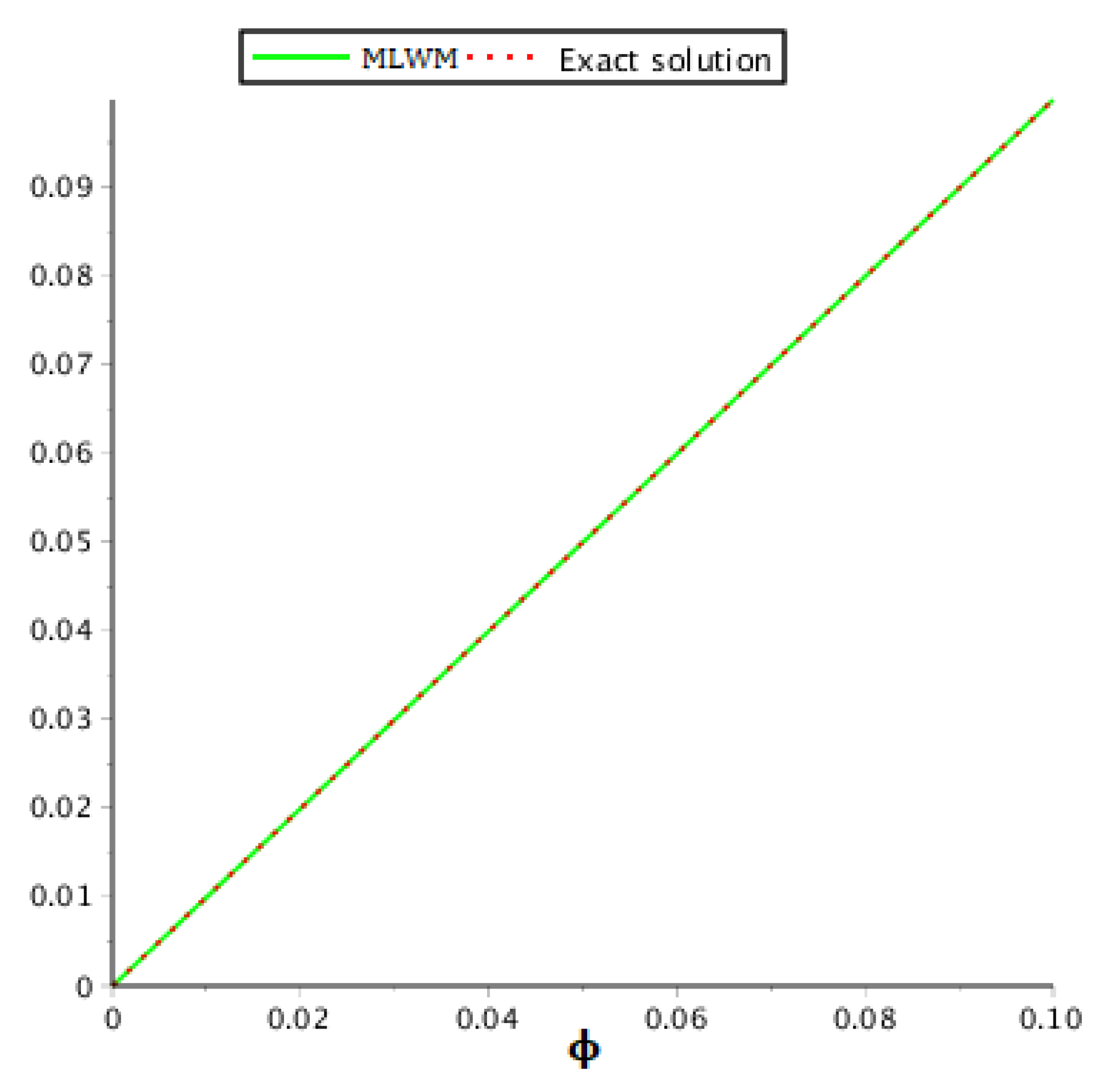
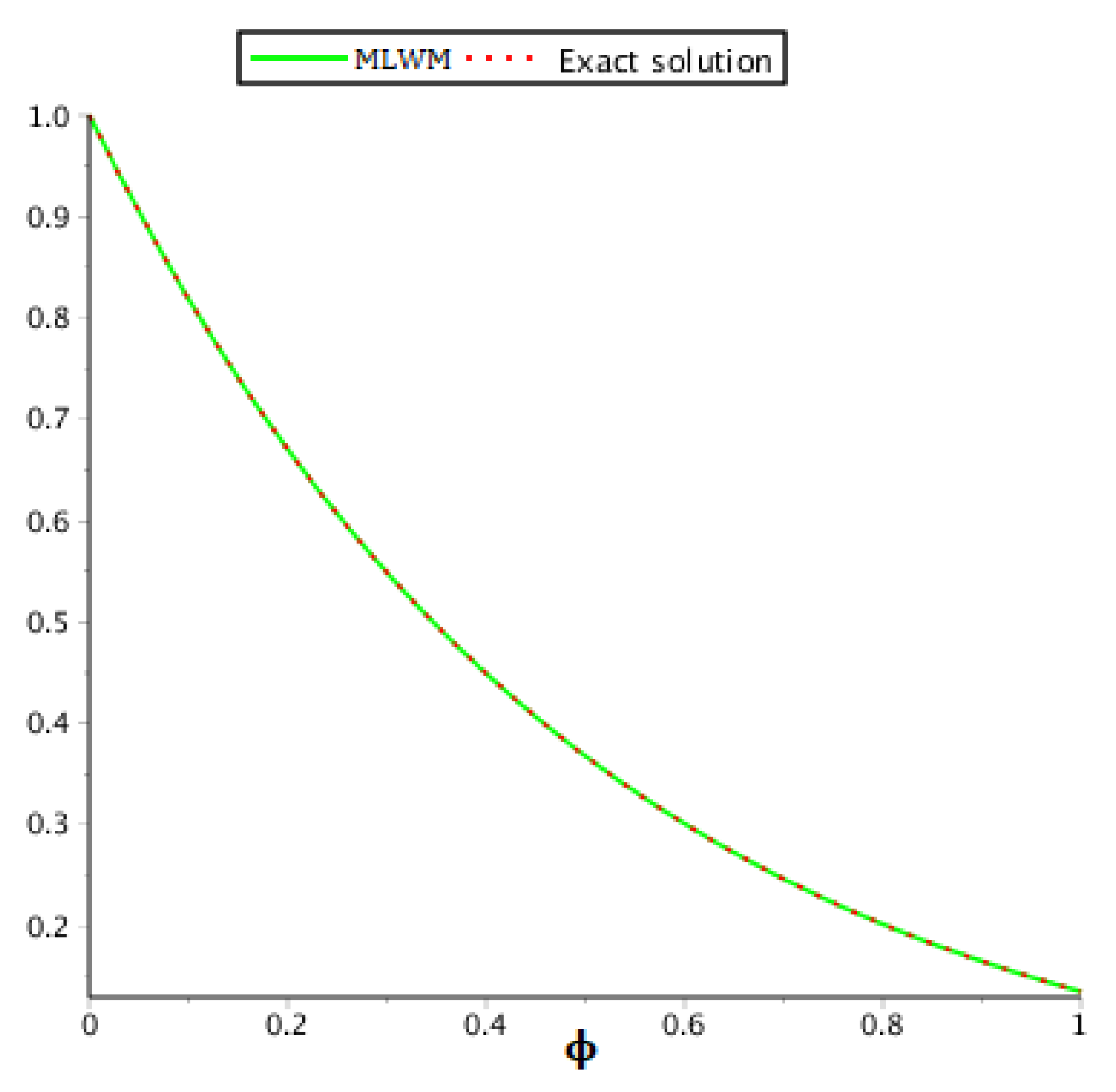
φ	Exact	MLWM	MLWM Relative Error	MLWM Absolute Error
0	0.000000000000000	0.000000000000000	1.4836795250 × 10−10	6.7400000000 × 10−11
$0.1$	$0.009999832986000$	$0.009999833334000$	$3.4800581220\times {10}^{-8}$	$3.4800000000\times {10}^{-10}$
$0.2$	$0.019998664680000$	$0.019998666690000$	$1.0050671040\times {10}^{-7}$	$2.0100000000\times {10}^{-9}$
$0.3$	$0.029995494540000$	$0.029995500200000$	$1.8869500530\times {10}^{-7}$	$5.6600000000\times {10}^{-9}$
$0.4$	$0.039989323110000$	$0.039989334190000$	$2.7707395720\times {10}^{-7}$	$1.1080000000\times {10}^{-8}$
$0.5$	$0.049979152080000$	$0.049979169270000$	$3.4394341010\times {10}^{-7}$	$1.7190000000\times {10}^{-8}$
$0.6$	$0.059963984300000$	$0.059964006480000$	$3.6988869670\times {10}^{-7}$	$2.2180000000\times {10}^{-8}$
$0.7$	$0.069942823940000$	$0.069942847340000$	$3.3455898230\times {10}^{-7}$	$2.3400000000\times {10}^{-8}$
$0.8$	$0.079914676470000$	$0.079914693970000$	$2.1898355560\times {10}^{-7}$	$1.7500000000\times {10}^{-8}$
$0.9$	$0.089878548870000$	$0.089878549200000$	$3.6716213620\times {10}^{-9}$	$3.3000000000\times {10}^{-10}$
$1.0$	$0.099833449630000$	$0.099833416650000$	$3.3035019950\times {10}^{-7}$	$3.2980000000\times {10}^{-8}$

. The results of the present method are compared with the discontinuous Galerkin (DG) approach [44] in

Table 2. Absolute errors comparison for Problem 1.

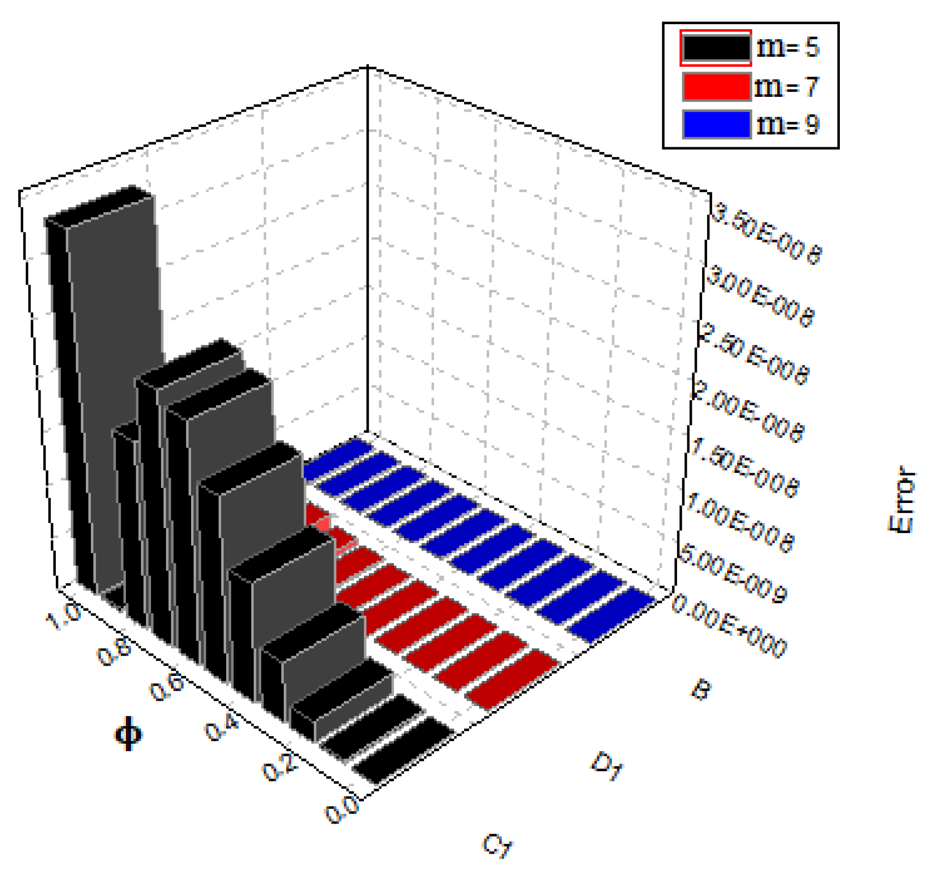
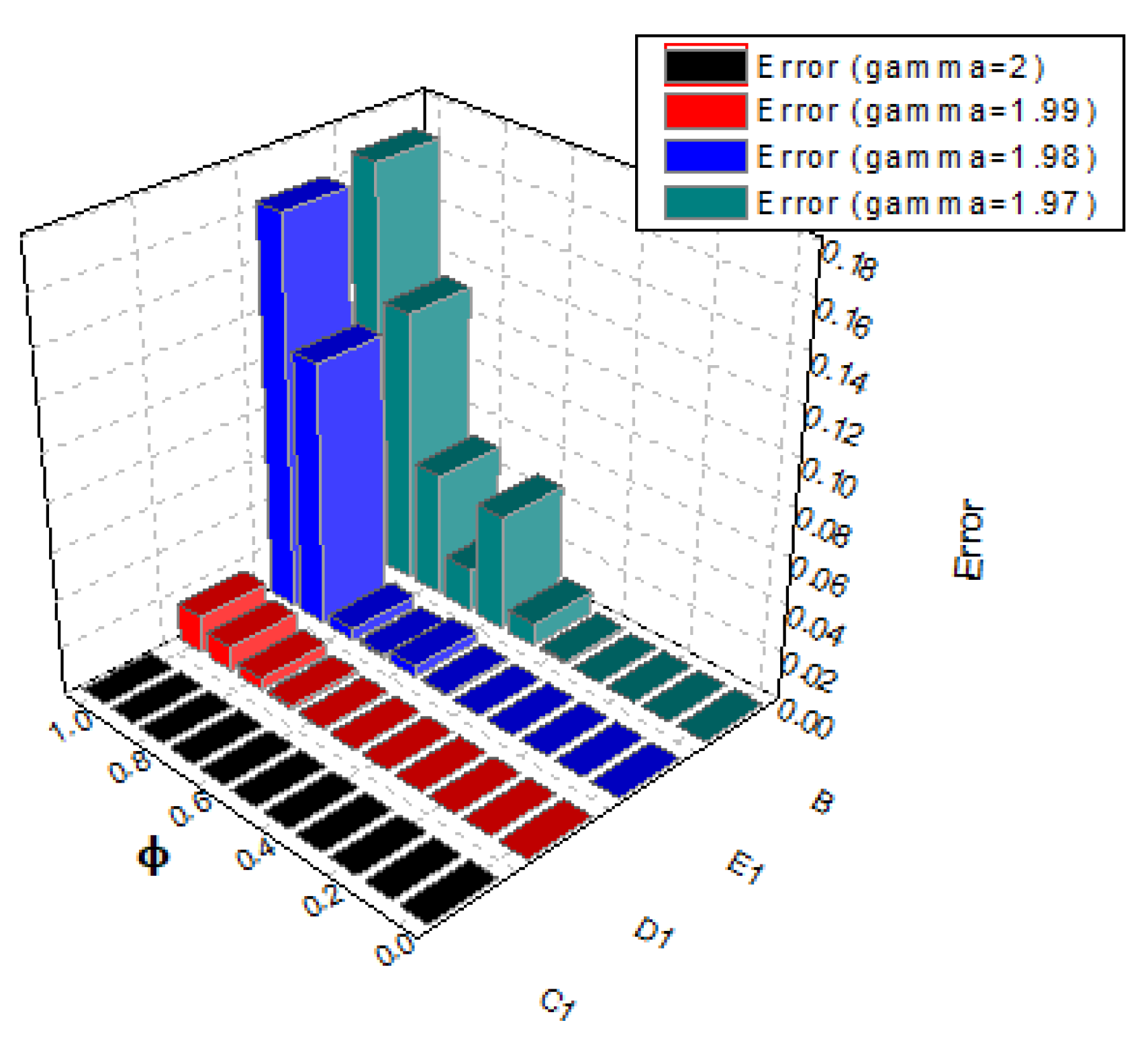
m	Piecewise Constant	Piecewise Linear	Piecewise Linear	TLM	MLWM
	DG at $\mathit{m}=64$	DG at $\mathit{m}=64$	DG at $\mathit{m}=16$	at $\mathit{m}=5$	at $\mathit{m}=5$
Error	$1.4032\times {10}^{-2}$	$2.1429\times {10}^{-5}$	$1.4643\times {10}^{-6}$	$3.8567\times {10}^{-7}$	$3.3000\times {10}^{-10}$

which confirm that MLWM shows quick convergence as compared to the DG method for this problem.

Problem 2. 

Assume the following FPDDE as

$$D_{\phi }^{\gamma }\mu \left(\phi \right)=\mu \left(\phi \right)-\frac{8}{q^2}{\mu }^2\left(\frac{\phi }{2}\right),0\le \phi \le 1,1<\gamma \le 2,0<q\le 1$$

(15)

with initial sources $\mu \left(0\right)=0$ and ${\mu }^{\prime }\left(0\right)=1$.

The exact solution at $\gamma =2$ is

$${\displaystyle \mu \left(\phi \right)=\phi exp\left(-\phi \right).}$$

The exact solution and MLWM results at $m=11$ are drawn in Figure 5. The exact solution, MLWM solution in addition to relative error and absolute error are given in

Table 3. Nature of Exact and MLWM solutions by means of relative error and absolute error for Problem 2.

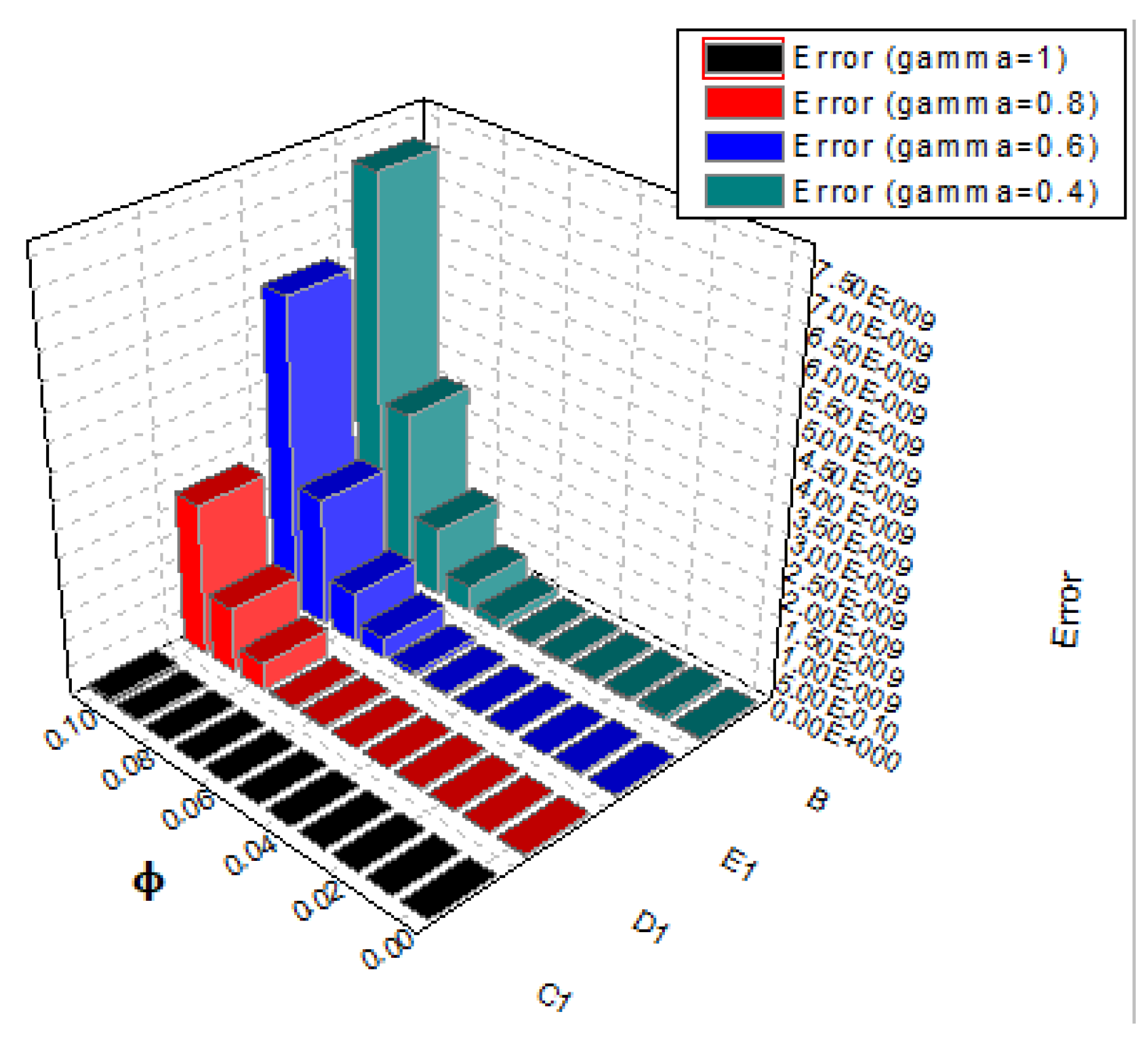
φ	Exact	MLWM	MLWM Relative Error	MLWM Absolute Error
0	$0.000000000000000$	$0.000000000000000$	1.4564072715 $\times {10}^{-18}$	$4.5787621700\times {10}^{-20}$
$0.1$	$0.090483741803596$	$0.090483741803596$	$2.3164095794\times {10}^{-17}$	$2.0959740630\times {10}^{-18}$
$0.2$	$0.163746150615598$	$0.163746150615596$	$1.0561631346\times {10}^{-14}$	$1.7294264772\times {10}^{-15}$
$0.3$	$0.222245466204594$	$0.222245466204515$	$3.5323561564\times {10}^{-13}$	$7.8505014078\times {10}^{-14}$
$0.4$	$0.268128018415322$	$0.268128018414256$	$3.9756559605\times {10}^{-12}$	$1.0659847546\times {10}^{-12}$
$0.5$	$0.303265329863632$	$0.303265329856317$	$2.4122404163\times {10}^{-11}$	$7.3154888555\times {10}^{-12}$
$0.6$	$0.329286981688216$	$0.329286981656416$	$9.6571254363\times {10}^{-11}$	$3.1799656867\times {10}^{-11}$
$0.7$	$0.347609712751709$	$0.347609712653987$	$2.8112532420\times {10}^{-10}$	$9.7721893193\times {10}^{-11}$
$0.8$	$0.359463171517328$	$0.359463171293777$	$6.2190241894\times {10}^{-10}$	$2.2355101589\times {10}^{-10}$
$0.9$	$0.365912694155867$	$0.365912693766539$	$1.0639912292\times {10}^{-9}$	$3.8932789723\times {10}^{-10}$
$1.0$	$0.367879441725032$	$0.367879441171442$	$1.5048121491\times {10}^{-9}$	$5.5358945331\times {10}^{-10}$

whereas

Table 4. Exact solution, MLWM solutions and MLWM absolute error comparison with MDTM for Example 2.

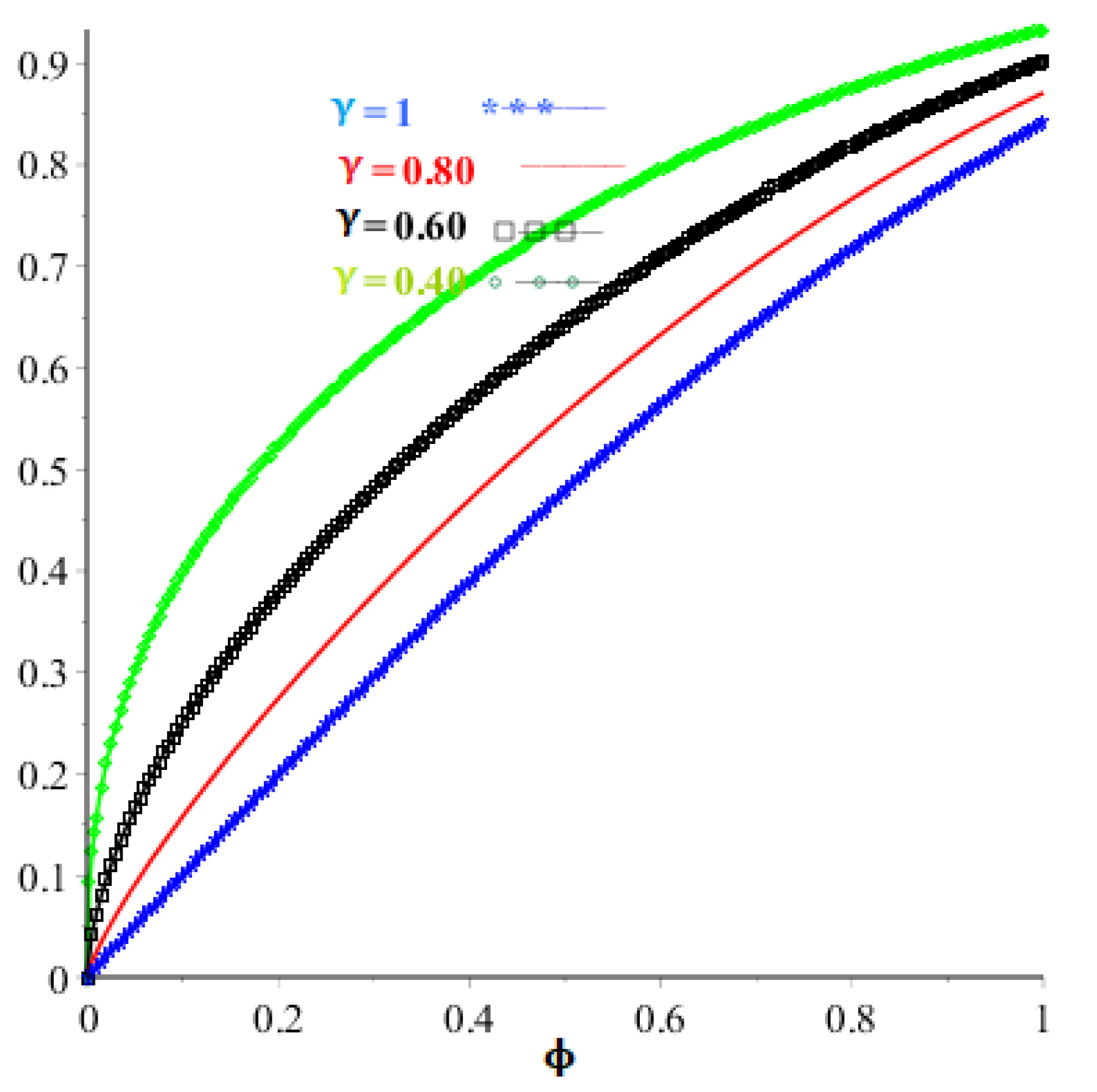
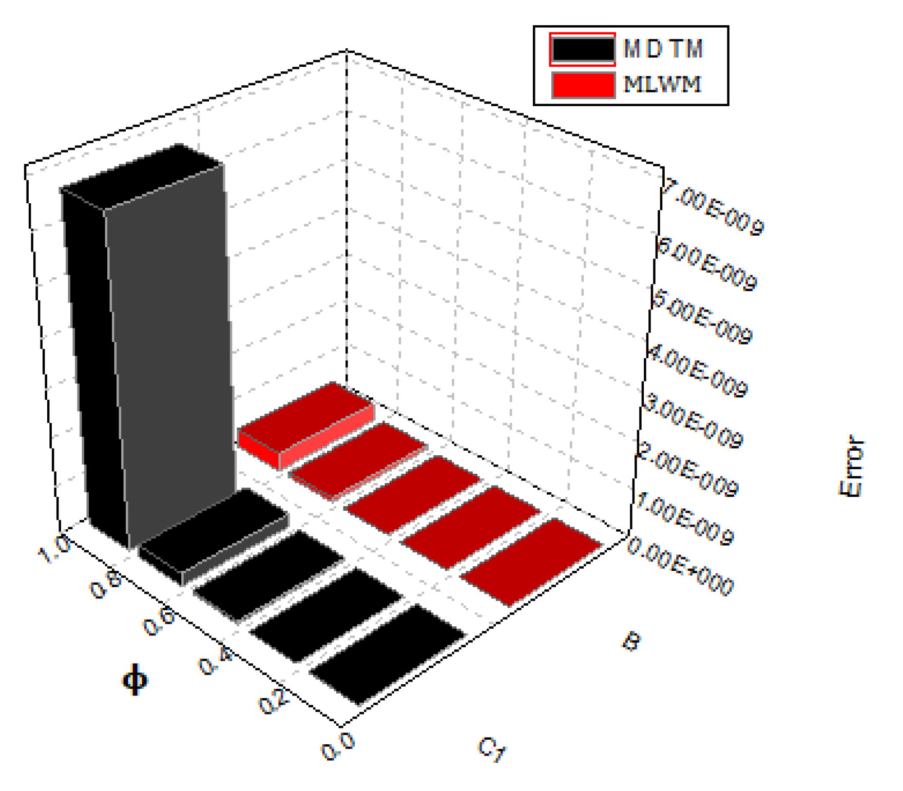
φ	Exact Solution	MLWM Solution	MDTM [50] Error	MLWM Error
$0.1$	$0.090483741803596$	$0.090483741803596$	3.592657686 $\times {10}^{-12}$	$2.0959740630\times {10}^{-18}$
$0.3$	$0.222245466204515$	$0.222245466204594$	$4.528351013\times {10}^{-12}$	$7.8505014078\times {10}^{-14}$
$0.5$	$0.303265329856317$	$0.303265329863632$	$5.85598678\times {10}^{-11}$	$7.3154888555\times {10}^{-12}$
$0.7$	$0.347609712653987$	$0.347609712751709$	$2.78563346\times {10}^{-10}$	$9.7721893193\times {10}^{-11}$
$0.9$	$0.365912693766539$	$0.365912694155867$	$6.64594981\times {10}^{-9}$	$3.8932789723\times {10}^{-10}$

gives the absolute error comparison of MLWM and MDTM at $m=11$ which confirms that MLWM converges rapidly as compared to MDTM. For the comparison, we take significant digits up to 20 to attain a more precise solution. In Figure 6, we demonstrate the error comparison of both approaches whereas the absolute errors at various fractional-orders are illustrated in Figure 7. Furthermore, the fractional-order solutions graph of the suggested technique are illustrated in Figure 8. The solutions of the proposed technique are in better agreement than the MDTM technique for this problem.

5. Conclusions

In this work, we applied the Modified Laguerre Wavelet approach to solve FPDDEs. The derivative is taken in the Caputo sense. The method is simple and exhibits a faster convergence rate than other methods. The proposed algorithm’s ability to smoothly convert from linear to nonlinear functionality presents one of its primary advantages. The method also has the benefit of simplifying the problem-solving process by transforming the nonlinear differential equation into a set of algebraic equations. Furthermore, values of m are used to achieve approximations with excellent precision. Examples are presented to show the usefulness and application of the suggested methodology. Several problems are solved to determine the effectiveness of the present approach. We obtain more precise results when m is increased, according to the numerical data provided herein. The results are compared with those obtained by various other methods such as the discontinuous Galerkin (DG) method, spectral method, transferred Legendre pseudospectral method and modified differential transform method. MLWM demonstrates superior accuracy over these techniques, as evidenced by the comparisons provided. Furthermore, the application of MLWM to various fractional delay or non-delay physics and real scientific models is a relatively simple task.

References

- Miller, K.S.; Ross, B. An Introduction to the Fractional Calculus and Fractional Differential Equations; Wiley: Hoboken, NJ, USA, 1993. [Google Scholar]
- Loverro, A. Fractional Calculus: History, Definitions and Applications for the Engineer; Rapport Technique; Department of Aerospace and Mechanical Engineering, Univeristy of Notre Dame: Notre Dame, IN, USA, 2004. [Google Scholar]
- Bagley, R.L.; Torvik, P.J. Fractional calculus in the transient analysis of viscoelastically damped structures. AIAA J. 1985, 23, 918–925. [Google Scholar] [CrossRef]
- Engheta, N. On fractional calculus and fractional multipoles in electromagnetism. IEEE Trans. Antennas Propag. 1996, 44, 554–566. [Google Scholar] [CrossRef]
- Oldham, K.B. Fractional differential equations in electrochemistry. Adv. Eng. Softw. 2010, 41, 9–12. [Google Scholar] [CrossRef]
- Kulish, V.; Lage, J.L. Application of fractional calculus to fluid mechanics. J. Fluids. Eng. 2002, 124, 803–806. [Google Scholar] [CrossRef]
- Mainardi, F. Fractional Calculus: Some Basic Problems in Continuum and Statistical Mechanics; Springer: Vienna, Austria, 1997. [Google Scholar]
- Meral, F.C.; Royston, T.J.; Magin, R. Fractional calculus in viscoelasticity: An experimental study, Commun. Nonlinear Sci. Numer. Simul. 2010, 15, 939–945. [Google Scholar] [CrossRef]
- He, J.H. Nonlinear oscillation with fractional derivative and its applications. Int. Conf. Vib. Eng. 1998, 98, 288–291. [Google Scholar]
- Lederman, C.; Roquejoffre, J.M.; Wolanski, N. Mathematical justification of a nonlinear integrodifferential equation for the propagation of spherical flames. Ann. Mat. Pura Appl. 2004, 183, 173–239. [Google Scholar] [CrossRef]
- Davis, A.R.; Karageorghis, A.; Phillips, T.N. Spectral Galerkin methods for the primary two-point bour problem in modeling viscoelastic flows. Int. J. Numer. Methods Eng. 1988, 26, 647–662. [Google Scholar] [CrossRef]
- Agrawal, O.P. A general formulation and solution scheme for fractional optimal control problems. Nonlinear Dyn. 2004, 38, 323–337. [Google Scholar] [CrossRef]
- Oustaloup, A. Fractional order sinusoidal oscillators: Optimization and their use in highly linear FM modulation. IEEE Trans. Circ. Syst. 1981, 28, 1007–1009. [Google Scholar] [CrossRef]
- Sun, H.; Zhang, Y.; Baleanu, D.; Chen, W.; Chen, Y. A new collection of real world applications of fractional calculus in science and engineering. Commun. Nonlinear Sci. Numer. Simul. 2018, 64, 213–231. [Google Scholar] [CrossRef]
- Oliveri, F. Lie symmetries of differential equations: Classical results and recent contributions. Symmetry 2010, 2, 658–706. [Google Scholar] [CrossRef] [Green Version]
- Tsamparlis, M.; Paliathanasis, A. Symmetries of differential equations in cosmology. Symmetry 2018, 10, 233. [Google Scholar] [CrossRef] [Green Version]
- Bibi, K. Particular solutions of ordinary differential equations using discrete symmetry groups. Symmetry 2020, 12, 180. [Google Scholar] [CrossRef] [Green Version]
- Diethelm, K.; Ford, N.J.; Freed, A.D. A predictor-corrector approach for the numerical solution of fractional differential equations. Nonlinear Dyn. 2002, 29, 3–22. [Google Scholar] [CrossRef]
- Abdeljawad, T.; Agarwal, R.P.; Karapinar, E.; Kumari, P.S. Solutions of the nonlinear integral equation and fractional differential equation using the technique of a fixed point with a numerical experiment in extended b-metric space. Symmetry 2019, 11, 686. [Google Scholar] [CrossRef] [Green Version]
- Xie, Z.; Feng, X.; Chen, X. Partial least trimmed squares regression. Chemom. Intell. Lab. Syst. 2022, 221, 104486. [Google Scholar] [CrossRef]
- Sahoo, S.; Saha Ray, S.; Abdou, M.A.M.; Inc, M.; Chu, Y.M. New soliton solutions of fractional Jaulent-Miodek system with symmetry analysis. Symmetry 2020, 12, 1001. [Google Scholar] [CrossRef]
- Esmaeili, S.; Shamsi, M.; Luchko, Y. Numerical solution of fractional differential equations with a collocation method based on Müntz polynomials. Comput. Math. Appl. 2011, 62, 918–929. [Google Scholar] [CrossRef] [Green Version]
- Liu, L.; Wang, J.; Zhang, L.; Zhang, S. Multi-AUV Dynamic Maneuver Countermeasure Algorithm Based on Interval Information Game and Fractional-Order DE. Fractal Fract. 2022, 6, 235. [Google Scholar] [CrossRef]
- Sunthrayuth, P.; Aljahdaly, N.H.; Ali, A.; Mahariq, I.; Tchalla, A.M. ψ-Haar Wavelet Operational Matrix Method for Fractional Relaxation-Oscillation Equations Containing-Caputo Fractional Derivative. J. Funct. Spaces 2021, 2021, 7117064. [Google Scholar] [CrossRef]
- Alaroud, M.; Al-Smadi, M.; Rozita Ahmad, R.; Salma Din, U.K. An analytical numerical method for solving fuzzy fractional Volterra integro-differential equations. Symmetry 2019, 11, 205. [Google Scholar] [CrossRef] [Green Version]
- Li, X. Numerical solution of fractional differential equations using cubic B-spline wavelet collocation method. Commun. Nonlinear. Sci. Numer. Simul. 2012, 17, 3934–3946. [Google Scholar] [CrossRef]
- Sunthrayuth, P.; Ullah, R.; Khan, A.; Kafle, J.; Mahariq, I.; Jarad, F. Numerical analysis of the fractional-order nonlinear system of Volterra integro-differential equations. J. Funct. Spaces 2021, 2021, 1537958. [Google Scholar] [CrossRef]
- Zheng, W.; Liu, X.; Yin, L. Research on image classification method based on improved multi-scale relational network. Peerj Comput. Sci. 2021, 7, 613. [Google Scholar] [CrossRef]
- Li, P.; Li, Y.; Gao, R.; Xu, C.; Shang, Y. New exploration on bifurcation in fractional-order genetic regulatory networks incorporating both type delays. Eur. Phys. J. Plus 2022, 137, 598. [Google Scholar] [CrossRef]
- Pappalardo, C.M.; De Simone, M.C.; Guida, D. Multibody modeling and nonlinear control of the pantograph/catenary system. Arch. Appl. Mech. 2019, 89, 1589–1626. [Google Scholar] [CrossRef]
- Li, D.; Zhang, C. Long time numerical behaviors of fractional pantograph equations. Math. Comput. Simul. 2020, 172, 244–257. [Google Scholar] [CrossRef]
- Vanani, S.K.; Hafshejani, J.S.; Soleymani, F.; Khan, M. On the numerical solution of generalized pantograph equation. World Appl. Sci. J. 2011, 13, 2531–2535. [Google Scholar]
- Bogachev, L.; Derfel, G.; Molchanov, S.; Ochendon, J. On Bounded Solutions of the Balanced Generalized Pantograph Equation; Springer: New York, NY, USA, 2008. [Google Scholar]
- Rahimkhani, P.; Ordokhani, Y.; Babolian, E. Numerical solution of fractional pantograph differential equations by using generalized fractional-order Bernoulli wavelet. J. Comput. Appl. Math. 2017, 309, 493–510. [Google Scholar] [CrossRef]
- Yang, C.; Hou, J.; Lv, X. Jacobi spectral collocation method for solving fractional pantograph delay differential equations. Eng. Comput. 2022, 38, 1985–1994. [Google Scholar] [CrossRef]
- Dehestani, H.; Ordokhani, Y.; Razzaghi, M. Numerical technique for solving fractional generalized pantograph-delay differential equations by using fractional-order hybrid bessel functions. Int. J. Appl. Math. Comput. Sci. 2020, 6, 9. [Google Scholar] [CrossRef]
- Rabiei, K.; Ordokhani, Y. Solving fractional pantograph delay differential equations via fractional-order Boubaker polynomials. Eng. Comput. 2019, 35, 1431–1441. [Google Scholar] [CrossRef]
- Shi, L.; Ding, X.; Chen, Z.; Ma, Q. A new class of operational matrices method for solving fractional neutral pantograph differential equations. Adv. Differ. Equ. 2018, 2018, 94. [Google Scholar] [CrossRef]
- Yuttanan, B.; Razzaghi, M.; Vo, T.N. A fractional-order generalized Taylor wavelet method for nonlinear fractional delay and nonlinear fractional pantograph differential equations. Math. Methods Appl. Sci. 2021, 44, 4156–4175. [Google Scholar] [CrossRef]
- Nonlaopon, K.; Naeem, M.; Zidan, A.M.; Alsanad, A.; Gumaei, A. Numerical investigation of the time-fractional Whitham-Broer-Kaup equation involving without singular kernel operators. Complexity 2021, 2021, 7979365. [Google Scholar] [CrossRef]
- Shiralashetti, S.; Kumbinarasaiah, S.; Naregal, S. Laguerre wavelet based numerical method for the solution of diferential equations with variable coefcients. Int. J. Eng. Sci. Math. 2017, 6, 40–48. [Google Scholar]
- Shiralashetti, S.; Angadi, L.; Kumbinarasaiah, S. Laguerre wavelet-Galerkin method for the numerical solution of one dimensional partial differential equations. Int. J. Math. Appl. 2018, 55, 939–949. [Google Scholar]
- Shiralashetti, S.; Kumbinarasaiah, S. Laguerre wavelets collocation method for the numerical solution of the Benjamina-Bona-Mohany equations. J. Taibah. Univ. Sci. 2019, 13, 9–15. [Google Scholar] [CrossRef] [Green Version]
- Shah, N.A.; Alyousef, H.A.; El-Tantawy, S.A.; Shah, R.; Chung, J.D. Analytical Investigation of Fractional-Order Korteweg-DeVries-Type Equations under Atangana-Baleanu-Caputo Operator: Modeling Nonlinear Waves in a Plasma and Fluid. Symmetry 2022, 14, 739. [Google Scholar] [CrossRef]
- Areshi, M.; Khan, A.; Nonlaopon, K. Analytical investigation of fractional-order Newell-Whitehead-Segel equations via a novel transform. AIMS Math. 2022, 7, 6936–6958. [Google Scholar] [CrossRef]
- He, J.H. Some applications of nonlinear fractional differential equations and their approximations. Bull. Sci. Technol. Soc. 1999, 15, 86–90. [Google Scholar]
- Bagley, R.L.; Torvik, P.J. A theoretical basis for the application of fractional calculus to viscoelasticity. J. Rheol. 1983, 27, 201e10. [Google Scholar] [CrossRef]
- Panda, R.; Dash, M. Fractional generalized splines and signal processing. Signal Process 2006, 86, 2340e50. [Google Scholar] [CrossRef]
- Shah, N.A.; Hamed, Y.S.; Abualnaja, K.M.; Chung, J.D.; Khan, A. A comparative analysis of fractional-order kaup-kupershmidt equation within different operators. Symmetry 2022, 14, 986. [Google Scholar] [CrossRef]
- Noori, S.R.M.; Taghizadeh, N. Modified differential transform method for solving linear and nonlinear pantograph type of differential and Volterra integro-differential equations with proportional delays. Adv. Differ. Equ. 2020, 2020, 649. [Google Scholar] [CrossRef]