
From Skyrmions to One Flavored Baryons and Beyond
Department of Applied Mathematics and Theoretical Physics, University of Cambridge, Cambridge CB3 OWA, UK
Symmetry 2022, 14(11), 2347; https://doi.org/10.3390/sym14112347
Submission received: 2 October 2022
/
Revised: 29 October 2022
/
Accepted: 3 November 2022
/
Published: 8 November 2022
(This article belongs to the Special Issue Symmetries and Ultra Dense Matter of Compact Stars)
Abstract
:While the identification of skyrmions as the low energy description of baryons in QCD is known for decades, a parallel construction for the case of is more mysterious. In the case of one fermionic flavor, there is no chiral symmetry breaking, no non-linear sigma model, and the conventional construction of skyrmions fails to work. In this article, I will review developments from the last couple of years trying to identify baryons as certain singular configurations in the large limit of QCD. We will give various arguments supporting this identification, and discuss some of its applications. Unlike skyrmions, the new baryons are not contained completely inside the low energy effective theory. They give rise to a singular ring on which the chiral condensate must vanish, with new degrees of freedom living on this ring. These configurations may serve as a bridge between the UV and the IR, and hopefully shed some light on the connection between different phases of QCD.
1. Introduction
QCD is a theory that we understand very well at two corners of its phase diagram. At very high energies, it is described as a weakly interacting gauge theory coupled to fundamental fermions. By assuming confinement and chiral symmetry breaking, the low energy theory is described as an non-linear sigma model with a level N Wess-Zumino (WZ) term [1,2]. The WZ term is fixed uniquely by anomaly matching conditions. This model, and in particular, the WZ term, are extremely successful in combining deep theoretical ideas with concrete measurements. The effective degrees of freedom in this regime are the pions, which are the Nambu–Goldstone (NG) bosons associated with chiral symmetry breaking, and baryons that appear as topological solitons in the effective theory of pions. Once we leave the deep infrared (IR) limit and increase the energy, we lose theoretical control over the physics. In addition to higher derivatives terms, a zoo of mesons come back to life, which results in many possible interactions. Ideally, we would like to find theoretical arguments that reveal a hidden order in the theory and restrict the space of couplings.
In this article, we will summarize recent developments in these directions involving in particular the meson, the vector mesons known as and , which we will denote collectively by V, and baryons constructed out of one fermionic flavor. We will show how advanced theoretical ideas based on higher-form symmetries and their anomalies, can be used to constrain some of the coupling of these mesons, and relate them to the low energy description of the one-favoured baryon. How are these three types of particles related? The most controlled way to add the to the chiral Lagrangian is by taking the large N limit. When N is large, the axial symmetry becomes a good symmetry of the theory. The spontaneous breaking of leads to an extra NG boson, which is the meson. Indeed, the mass of the field is suppressed in the large N limit, [3,4]. For the vector mesons, there are two phenomenological principles that are commonly used when writing their effective theory. The first is the hidden local symmetry (HLS) principle [5,6] which will be reviewed in Section 5, and the second is Vector Dominance (VD) [7,8] which will be reviewed in Appendix A. These two principles restrict the space of couplings and increase the predictive power of the theory. Yet, a good theoretical explanation for why these principles are correct is absent. The question of how a baryon in QCD can be described in terms of low energy degrees of freedom was an open question until the work of Komargodski in [9]. Later, this construction was elaborated and further studied in several papers, such as [10,11,12,13,14,15,16,17]. It was shown that there exist singular configurations that carry baryon charge. Such configurations look like a finite surface that connects on one side to on the other (recall that is the phase of the chiral condensate and as such, is periodic). The boundary of this surface is a singular ring on which is not well defined and the chiral condensate is expected to vanish. New degrees of freedom living on the singular ring carry baryon charge. Hence this entire configuration is a baryon. It has been conjectured that these new mysterious degrees of freedom are actually the vector mesons mentioned above. Hence, the baryon is a singular soliton constructed out of and the vector mesons. It happens to be that for this construction to work appropriately, one needs to fix two coupling constants between pions, , and vector mesons to take specific values, . Unlike the coefficient of the WZ term, which is fixed to be by anomalies, so far there has been no good theoretical argument fixing the values of these parameters. Surprisingly, this is exactly the value predicted by VD. Thus, the construction of baryons provides a theoretical explanation to the phenomenological observation of VD, and VD provides an experimental evidence supporting the construction of baryons. The outline of this article is as follows. In Section 2, we review basic facts about skyrmions, and the motivation for identifying them with the low energy description of baryons. In Section 3, we study qualitatively what happens to a skyrmion as we change the mass of one of the quarks and continuously flow from QCD to QCD. Since the baryon charge is preserved along the way, the final configuration should be similar to the low energy description of baryons in QCD. In Section 4, we move on to study directly the construction of baryons in QCD. We will review the proposal made in the literature and give some evidence supporting this proposal. In Section 5, we add the vector mesons to the theory and show how their contribution to the baryon current enables us to write a unified current under which both the conventional skyrmions and the new baryons are charged. We also derive the conditions on the parameters mentioned above. In Appendix A, we review the principle of VD and show agreement between it and the conditions derived in Section 5.
2. Skyrmions: Review
In this section, we will review some of the basic facts about skyrmions. The content of this section appears in many papers and textbooks; see for example, [18,19,20,21,22,23,24,25,26,27,28,29]. Our starting point is QCD with massless Dirac fermions. The theory enjoys the global symmetry (We consider here only the continuous symmetries. See for example, [30] for a discussion about the discrete factors.) of . In addition, the QCD Lagrangian enjoys the axial symmetry which is broken by non-perturbative effects. However, in the large N limit, the symmetry is restored and becomes an exact symmetry of the theory. For not too large (below the conformal window), the theory is confining at low energies, and the symmetries are spontaneously broken by the chiral condensate
where is the diagonal subgroup of , leaving the chiral condensate invariant. The low energy effective theory can be described using the Goldstone theorem via a non-linear sigma model, parametrized by . The global symmetries act on U as
where parametrizes . Indeed, the vacuum breaks the symmetries as described in (1). , on the other hand, does not act on U. From the microscopic point of view, the only gauge invariant operators charged under are the baryons
where are the color indices and are the flavor indices. A surprising fact about baryons is that even though we wrote an effective theory only for the massless Nambu–Goldstone (NG) modes and threw away all the rest, baryons still appear as solitons, which are famously known as skyrmions. The effective theory is described using the chiral Lagrangian
The ⋯ includes higher derivatives terms, and for , also the Wess-Zumino term [1,2]; see Section 5 for a review. For any finite energy configuration, the fields must go to their vacuum at infinity . Finite energy configurations are maps from to , which are classified by
which allows for the existence of stable solitons. The associated topological current is the skyrmion current
which is the identically conserved , and the associated charge is . We will focus now on the simple case of . A convenient parametrization of is
where are the Pauli matrices. An example for a charged configuration is the hedgehog ansatz
The condition can be satisfied by taking without a loss of generality. Demanding that U has a well defined limit at the origin requires to vanish, which implies for some integer K. It is a straightforward exercise to show that for this configuration
There are many pieces of evidence and consistency checks showing that the skyrmions indeed should be identified with baryons, and that the topological symmetry (6) is the low energy description of . These include the spin, coupling to chiral gauge fields, large N, and many more. We will elaborate on some of them in the next sections. For any , the story works basically the same by choosing an and embedding the hedgehog solution in this subgroup.
2.1. Skyrmions from Anomalies
One of the strongest evidence that skyrmions are indeed the low energy description of baryons comes from anomalies. The anomaly we want to discuss here is the mixed triangle anomaly between and (or alternatively, ). In the UV, there are N quarks in the fundamental representation of , and charge under . This results in a triangle anomaly with coefficient 1. Another way to phrase the anomaly is that if we turn on the background gauge fields for , the baryon current obeys the equation
where is the background field strength for . An immediate consequence of this equation is that if we turn on such that on some time slice, , the vacuum in this background carries baryon charge 1. How is this anomaly realized in the IR? Consider the skyrmion current . The topological associated with this current has mixed anomalies with . To see it, couple to background gauge fields . The covariant derivative of U becomes . One can show that it is impossible to write a conserved gauge invariant current for , which means that if we gauge , is broken. Hence, there is a mixed anomaly between them. The best that we can achieve is to define the current
is not conserved, but it satisfies , which is the same as (10) if we identify the skyrmion current with the baryon current. Indeed, if we turn on , such that , the vacuum of this configuration will have a baryon charge of 1. This is satisfied because the vacuum equation is , which immediately gives
in agreement with the identification of the skyrmion current and the baryon current.
2.2. Skyrmions from Large N
Another evidence for this identification comes from large N, as was shown in [2]. The prescription of [2] to derive the baryon current in the chiral Lagrangian is as follows:
- 1.
- Compute the Noether current for a general vector-like symmetry that acts asThis can be achieved by coupling the symmetry to a gauge field A and reading the current from the term in the Lagrangian.
- 2.
- After deriving , plug in . U is invariant under this transformation . Therefore, most of the contributions to will vanish.
- 3.
- The only exception is the contribution coming from the 5D WZ term. This is due to some extra integration by parts when going from 5D to its 4D boundary, which changes the relative sign between two terms.
- 4.
- As a result, the baryon current is given by the skyrmion current
One might be suspicious about the degree of rigorousness of this derivation, since U is not charged under , and this “limit” is ambiguous. However, at least in the large N limit, we can justify this derivation. The reason for is that in the large N limit, becomes an approximate symmetry, the target space is enlarged from to , and we can take . In this case, we can really approach continuously, and obtain the skyrmion current, no matter how the limit is taken.
3. Flow
Before we attack the problem of baryons in QCD directly, we will try to continuously modify QCD to QCD by continuously changing the mass of one of the quarks from 0 to ∞. When doing so, we expect the mass difference between the skyrmion and the one-flavored baryon to decrease, until at some point when the second quark is very massive, the one-flavored baryon is expected to minimize the energy within the topological sector defined by . In the extreme limit, where the mass of the second quark , the microscopic theory flows to QCD, and the one-flavored baryon remains the only baryon in the spectrum. To achieve this, we will enlarge the target space from to with the following parametrization
The matrix U is invariant under
For simplicity, we will take for now the large N limit where is massless and treat it as a NG boson; however, nothing qualitative is expected to be different for finite N, where an explicit mass term for is introduced.
Our next step will be to add a mass term for the second quark. When the mass is small, the effect is to add to the chiral Lagrangian the following term
where we took the mass matrix
As a result, three of the four NG bosons become massive. The mass term vanishes for and .
For a configuration with a non-trivial skyrmion charge, we cannot simply take all the massive fields to zero. It is obvious from the expression for the current (6) that we need the three pions in order to obtain a non-trivial charge. For small mass, the hedgehog solution will be deformed in some small way to minimize the energy. If the mass of the down quark is very large, the solution will be highly deformed in a way that minimizes the volume in which the massive fields are non-zero. The first thing is that we can turn on a value for . does not enter into the skyrmion current and we can use it to cancel at least some of the mass contribution. This is achieved by choosing
Notice that with this choice, the bottom-right entry of U is exactly 1. Is this choice of well defined? The denominator in (19) is zero when . Do such points exist in the skyrmion solution? For the hedgehog, it happens on the ring defined by . Actually, this ring is a topological invariant in the sense that any topologically non-trivial mapping from to must include a ring on which . What about ? From the hedgehog solution, we see that are zero at and on the z-axis. The regime in which they do not vanish has the shape of a bead, which can be continuously deformed to a ring, the same ring on which . We see that we can push all the massive fields to the ring, where outside the ring only the massless NG field is excited. We can suggest the following ansatz for the skyrmion solution in the large limit,
where is as usual the angular coordinate along the ring; h equals on the ring and goes to zero very fast outside of the ring, winds once around the ring from 0 to . (When continuously deforming the hedgehog to (20), it can be seen that is roughly . f is even under , and as you go around the ring, it varies from 0 to and back to 0 without any winding. , on the other hand, winds once from 0 to .) The equation in (20) carries the non-trivial topological charge , and it is a continuous deformation of the hedgehog solution. The behavior of is presented in Figure 1.
We see that as we flow to , the skyrmion transforms continuously to a configuration in which winds around a singular ring. The winding of along the ring should be replaced by a winding of some new degree of freedom that appears on the singular ring. In the next section, we will present an alternative construction of this baryon directly from QCD, based on [9].
4. Quantum Hall Droplet: Review
In this section, we will review the recent work by Komargodski [9] in which he constructed a soliton that can identified with the baryon. From the microscopic point of view, baryons can be written as
Due to the anti-symmetrization over color indices, and the fermionic nature of , the spin indices must be symmetrized over to obtain something that is not identically zero. Therefore, there exists only one type of baryon, and its spin is . The low energy effective theory is gapped. However, as mentioned above, in the large N limit, becomes an exact symmetry, and its breaking leads to a NG boson known as the . is a periodic scalar, . The effective Lagrangian including the leading correction is given by
The potential term is locally quadratic, but it has a cusp whenever . For small fluctuations around the vacuum , it simply looks like a mass term, but when global effects that include the non-trivial winding of are present, the cusp plays an important role. The physical interpretation of the cusp is that when crosses , heavy fields jump from one vacuum to the other [31]. As one crosses the cusp, for example, by constructing a domain wall connecting and , the surface in the middle supports a QFT living on its worldvolume. It has been argued that this QFT should include a Chern–Simons (CS) theory. The appearance of this CS term is closely related to the first-order phase transition in pure Yang–Mills theory (YM) when [3,31,32,33,34]. The simplest way to see this is to notice that due to the ABJ anomaly, axial transformations lock shifts of by a constant with shifts of by the same constant . YM at has a mixed ’t-Hooft anomaly between time reversal symmetry and the center one-form symmetry. (We use here the notation of [35] where p-form symmetry acts on p-dimensional objects and is described by (d-p-1)-dimensional charges (where d is the dimension of spacetime). For example, zero-form symmetries are ordinary symmetries that act on local operators and are described by dimensional charges. One-form symmetries act on line operators, which are the Wilson lines in the case of YM, and so on. We refer the reader to [35] for more details.) The domain wall connects two vacua related by the action of time reversal, which implies that the theory on the domain wall must carry an anomalous one-form symmetry. The desired anomaly is matched by the Chern–Simons (CS) theory. (There is also a dual description in terms of an CS theory, but for us, the first description will be more convenient.)
The theory (23) enjoys a topological two-form symmetry, associated with the current
This symmetry is emergent in the IR and does not come from any UV symmetry. Charged objects under this symmetry are infinitely extended sheets that interpolate from on one side to on the other [36,37]. As an example, consider the configuration
Indeed, the configuration satisfies. (Notice that because this is a two-form symmetry, the charge is codimension 3. See [35] for more details.)
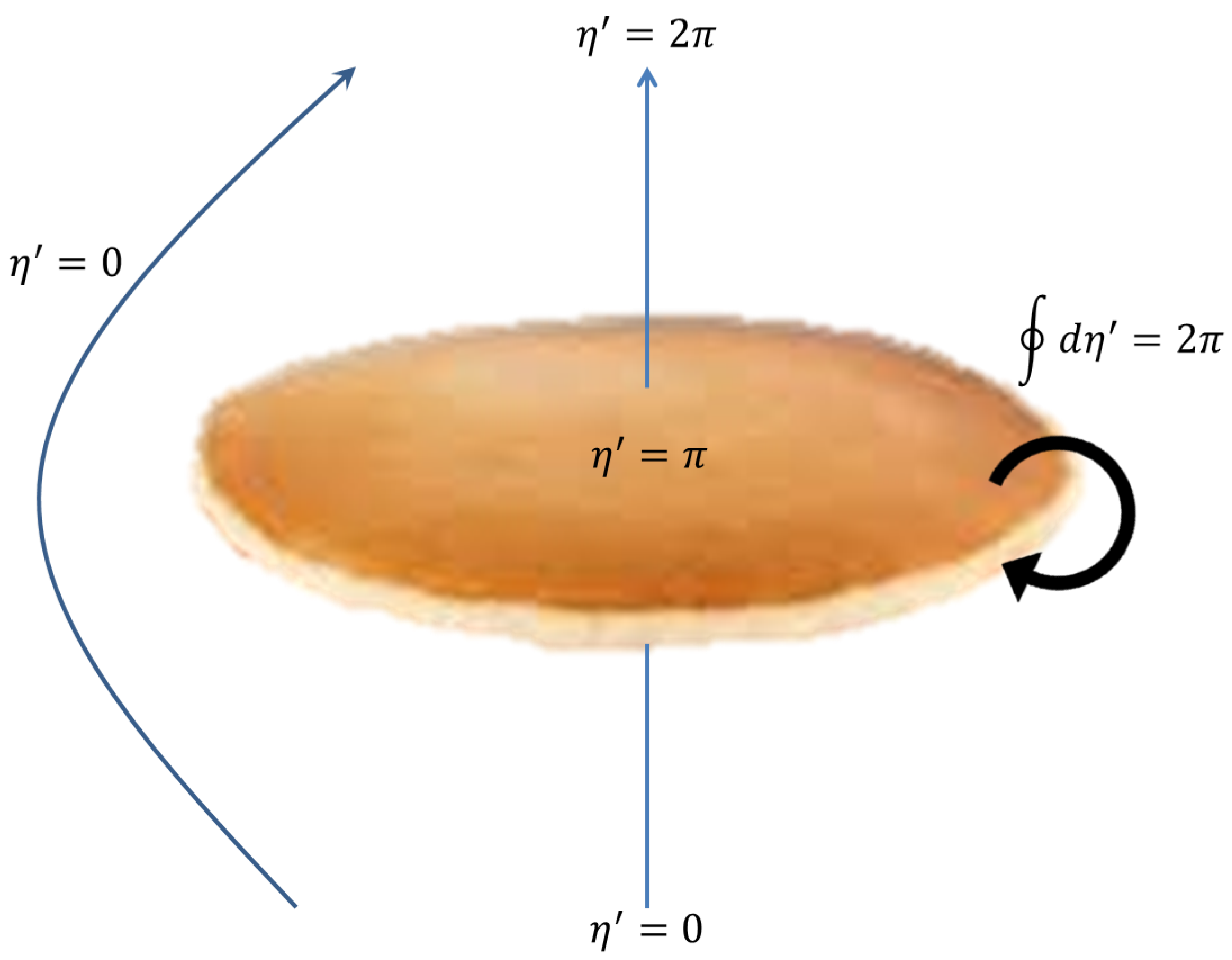
One problem with these sheets is that while their tension is finite, their mass ∼ diverges. One cannot construct finite energy configurations charged under this symmetry in 3+1 dimensions. Instead, we can consider finite sheets of the following schematic form. To obtain finite energy, we must demand that . In addition, we will try to impose that as before, with . These two demands cannot live together without having singularities somewhere in space. The minimal singularity that must exist is of the form of a ring surrounding the sheet. The configuration is illustrated in Figure 2, where it can be seen that must wind from 0 to as we go around the ring.
A key question is what happens on the ring. We can expect that as we go closer and closer to the ring, the chiral condensate goes to zero until it vanishes exactly on the ring. The physics on the ring is therefore beyond the scope of the low energy effective theory (23). A progress can still be made if we think of the ring as the boundary of the CS theory living on the sheet. A dimensional theory of a CS theory with a boundary has been well studied, especially in the context of the Quantum Hall effect. See for example, [38] for a detailed review. We will give here the main points relevant to our discussion. Consider the CS theory on a disc of radius 1,
Under a general variation , the action transforms as
where is the angular coordinate on the boundary. For the specific choice of gauge variations , the transformation of the action is
The theory can be quantized as follows. In order to have a well defined variational principle, we impose Dirichlet boundary conditions, , such that the boundary term in (28) vanishes identically. In addition, Lorentz invariance leads us to choose . Gauge invariance then implies that on the boundary,
The bulk term in (28) gives the equations of motion (EOM), . The EOM are solved by having everywhere. However, can still be non-trivial. For example, we can allow configurations with non-trivial winding . The configuration can be continued to the bulk smoothly while keeping except for one singular point. For , this singular point is nothing but an invisible “Dirac point” (the 2D analogue of a Dirac string). We can extend the boundary conditions to the bulk by choosing the gauge . Fixing the gauge and plugging into the action, one obtains
The result is that the theory is described by a chiral compact boson living on the boundary. Going back to our theory, we found that there is a chiral boson living on the ring. By coupling the theory to a background gauge field for the baryon symmetry, it can be shown that the baryon charge should be equivalent to the winding of the boson
The configuration can be argued to be dynamically stable. There are various contributions to the energy of the configuration. Denote the radius of the ring by R. The potential for contributes energy proportional to the area of the disc ∼. The vanishing of the VEV of the chiral condensate on the ring contributes energy that is proportional to the perimeter of the ring ∼R. Finally, the edge mode contributes ∼ due to its momentum on the ring. While the first two contributions want to minimize R, the last one prefers to increase it, resulting in some finite radius.
The spin of this configuration can be shown to be precisely . The most convenient way of achieving this is in terms of the two-dimensional chiral theory living on the ring’s worldsheet. The operator carrying one unit of baryon charge is the vertex operator whose spin is . Interestingly, in addition to , the theory contains also which carries a fractional baryon charge. The appearance of this operator can be interpreted as having liberated quarks on the ring, that also carry a baryon charge. See also [15] for a more elaborated discussion on this point. This is a summary of some of the main results of [9]. We see that the construction described in this section is in agreement with the continuous flow described in Section 3. The new degree of freedom that appears on the ring (replacing as ) is the chiral boson that comes from having a CS theory with a boundary.
In the next section, we will give a more phenomenological perspective on the appearance of the CS term by introducing the vector mesons into the theory.
5. Vector Mesons and Hidden Local Symmetry
In this section, we will add the vector mesons to the chiral Lagrangian as gauge bosons for a hidden local symmetry. We will show that for a certain choice of parameters, the vector mesons couple to the pions and to in a way that allows us to identify them as the CS fields on the domain wall. As a result, the vector mesons play an essential role in the construction of the baryon. It is the winding of the vector mesons along the singular ring that carries baryon charge. We will begin by reviewing the WZ action. The WZ action can be written as [2]
with
where is the matrix of pions. Here and later, there is an implicit trace in flavor space, and all the forms are assumed to be contracted with the ∧ product. The integration is over a five-dimensional manifold whose boundary is the four-dimensional world . Miraculously, the theory does not depend on the fifth dimension for every in (33), thanks to
for every closed manifold . The integer is fixed to be the number of colors N via anomaly matching conditions. While (33) is uniquely fixed at low energies, we want to study a more fundamental theory and include in addition to pions, also the vector mesons. Any consistent action that reduces to (33) when integrating out the vector mesons is a possible “orange” completion (as opposed to UV completion; here, we are just a little bit above the infrared). We will introduce the vector mesons into the chiral Lagrangian using the idea of hidden local symmetry, and classify the space of allowed completions for the WZ term.
In the hidden local symmetry principle, we write U as a product of two unitary matrices
where the redundant transformations with are coupled to the dynamical gauge fields V, which transform as . In addition, the global symmetries act as
We also introduce the covariant derivative and the field strength
A convenient shorthand notation that we will use throughout the paper is
The most general two derivatives Lagrangian consistent with the above symmetries is
where a is some dimensionless free parameter and g is the coupling constant.
In the unitary gauge , this is written as
In addition to the usual kinetic terms for the pions and the vector fields, the Lagrangian contains a mass term for the vector fields with ∼, and interactions between the vectors and the pions. Now, we will present the most general hWZ action in the theory. By hWZ action, we mean all the terms whose Lorentz indices are contracted using the tensor, similar to (33). In addition, we demand that the action is gauge invariant under the hidden gauge transformations, consistent with the global symmetries (37) and with time reversal symmetry that acts on the fields as
We will also simplify the action by taking the large N limit in which only single trace (in flavor space) operators are considered. The most general hWZ Lagrangian that can be added to (33) is [39]
with . It is straightforward to verify that in the deep IR, upon integrating out the vector mesons by replacing , , and we are left only with (33), as expected. Explicitly, we can write (43) as
In this prescription, there is a family of consistent hWZ actions parameterized by three real numbers . In addition, we can couple the theory to a (dynamical or background) gauge field for some global ,
Here, Q is the diagonal matrix of charges, and A is the gauge field. Two important cases that we will discuss are when A is the photon (see Appendix A), and when A is a background field (see Section 5). When A is included, we need to redefine the covariant derivative accordingly,
The WZ action is modified due to this gauging in several ways. First, all the covariant derivatives in (43) should be replaced with . Second, there are two (not gauge invariant) four-dimensional terms that should be added to (33) in order to maintain gauge invariance, as was shown in [2]. Notice that the derivatives in (33) are not replaced by covariant derivatives in this formalism. Third, there is a freedom to add to the hWZ action, the gauge invariant 4D term
with .
Understanding which completion is the correct one is important, both from the theoretical and phenomenological points of view. As we will see next, the hWZ action contributes to the baryon current and to the coupling between and the vector mesons. If we want to identify the vector mesons with the emergent CS fields living on the sheet, and to obtain the correct baryon charge consistent with the construction of the previous sections, we must choose to
We will start from the coupling of and the vector meson . The hWZ action for QCD is highly simplified to
Taking a domain wall configuration of the form
the contribution coming from (49) to the effective domain wall theory is exactly,
For the special choice of , we exactly obtain a CS term where the vector meson is the CS vector field. Next, we will repeat the derivation of the skyrmion current performed in Section 2.2, for the full hWZ action. We start by computing the current associated with the transformation
and take in the end. At this point the covariant derivative of is
We also accompany this transformation with the gauge transformation
such that are themselves invariant under . This is achieved by modifying , such that the covariant derivative now becomes
Indeed, with this choice, the gauge field does not appear in the covariant derivative of . Now, we can compute the baryon current. We already know that (33) gives rise to the skyrmion current (14). We will compute the contribution from the hWZ action (43), including the improvement term (47). The terms proportional to and in (43) do not contribute to the baryon current because A does not appear in the covariant derivatives , as explained above. We do obtain contributions from due to the shift . In addition, the improvement term contains A explicitly. Together, we have
such that the full baryon current is
In the limit, we can integrate out the vector mesons and obtain
as expected. In addition, it has been shown in [10] that H and S differ only by a total derivative term and therefore give rise to the same charge for any smooth configuration. Except for the definition of the local current density, the only physical difference between S and B comes when computing the baryon charge of singular configurations, such as the baryons described above. In particular, for , the baryon current B can be written as
In Appendix A, it is shown that the principle of VD implies . With this choice, , and at , it simplifies to
An example of a charged configuration is our baryon [9]. The baryon charge of this configuration comes from the two orthogonal windings—the winding of around the ring, and the winding of the CS field along the ring (the edge mode). Equation (62) hints that the CS field on the DW is actually the vector meson. Indeed, configurations characterized by two orthogonal windings of the form
have integer baryon charge under (62),
where the integration is over the 3D space.
This quantization of charge fails to work for generic in (61). The charge is properly quantized for . Together with the condition found above, we have .
These arguments give new theoretical predictions for the values of the coupling constants in the effective theory of vector mesons. (See [13] for more arguments fixing also .)
Surprisingly, as reviewed in Appendix A, these conditions are exactly the ones predicted by VD, and are consistent with experimental results.
Funding
This research is supported by the STFC consolidated grant ST/P000681/1 and the EPSRC grant EP/V047655/1 “Chiral Gauge Theories: From Strong Coupling to the Standard Model”.
Institutional Review Board Statement
Not applicable.
Informed Consent Statement
Not applicable.
Data Availability Statement
Not applicable.
Conflicts of Interest
The author declares no conflict of interest.
Appendix A. Intrinsic Parity and Vector Dominance
One of the most important features of the WZ term is that this is the only term that breaks the intrinsic parity . As a result, various odd processes in QCD are fixed by the WZ term. The most famous are the scattering of two kaons to three pions , the decay of to two photons , and the four-vertex involving . These three do not involve vector mesons as one of the external particles, and the leading contribution indeed comes from coupled to the photon [2]. Other processes that contain vector mesons are, for example, and .
Vector dominance (VD) [7] is a related phenomenological principle that states that when vector mesons are included, some vertices do not appear explicitly in the Lagrangian and the contribution to them is dominated by an exchange of the internal vector meson. The study of VD from the hWZ action was considered commonly in the literature; see for example [8,39]. In this section, we will show that VD for the vertices and implies (48), where A in this section plays the role of the photon. We are interested in studying the effective vertices obtained from expanding U around the identity,
References
- Wess, J.; Zumino, B. Consequences of anomalous Ward identities. Phys. Lett. B 1971, 37, 95–97. [Google Scholar] [CrossRef] [Green Version]
- Witten, E. Global Aspects of Current Algebra. Nucl. Phys. 1983, B223, 422–432. [Google Scholar] [CrossRef]
- Witten, E. Current Algebra Theorems for the U(1) Goldstone Boson. Nucl. Phys. 1979, B156, 269–283. [Google Scholar] [CrossRef]
- Veneziano, G. U(1) Without Instantons. Nucl. Phys. 1979, B159, 213–224. [Google Scholar] [CrossRef] [Green Version]
- Bando, M.; Kugo, T.; Uehara, S.; Yamawaki, K.; Yanagida, T. Is rho Meson a Dynamical Gauge Boson of Hidden Local Symmetry? Phys. Rev. Lett. 1985, 54, 1215. [Google Scholar] [CrossRef]
- Bando, M.; Kugo, T.; Yamawaki, K. Nonlinear Realization and Hidden Local Symmetries. Phys. Rept. 1988, 164, 217–314. [Google Scholar] [CrossRef]
- Sakurai, J.J. Vector mesons 1960–1968. Lect. Theor. Phys. A 1969, 11, 1–22. [Google Scholar]
- Fujiwara, T.; Kugo, T.; Terao, H.; Uehara, S.; Yamawaki, K. Nonabelian Anomaly and Vector Mesons as Dynamical Gauge Bosons of Hidden Local Symmetries. Prog. Theor. Phys. 1985, 73, 926. [Google Scholar] [CrossRef] [Green Version]
- Komargodski, Z. Baryons as Quantum Hall Droplets. arXiv 2018, arXiv:hep-th/1812.09253. [Google Scholar]
- Karasik, A. Skyrmions, Quantum Hall Droplets, and one current to rule them all. arXiv 2020, arXiv:hep-th/2003.07893. [Google Scholar] [CrossRef]
- Kan, N.; Kitano, R.; Yankielowicz, S.; Yokokura, R. From 3d dualities to hadron physics. arXiv 2019, arXiv:hep-th/1909.04082. [Google Scholar] [CrossRef]
- Kitano, R.; Matsudo, R. Vector mesons on the wall. J. High Energy Phys. 2021, 3, 23. [Google Scholar] [CrossRef]
- Karasik, A. Vector dominance, one flavored baryons, and QCD domain walls from the ”hidden” Wess-Zumino term. SciPost Phys. 2021, 10, 138. [Google Scholar] [CrossRef]
- Karasik, A. Anomalies for anomalous symmetries. J. High Energy Phys. 2022, 2, 64. [Google Scholar] [CrossRef]
- Ma, Y.L.; Nowak, M.A.; Rho, M.; Zahed, I. Baryon as a Quantum Hall Droplet and the Cheshire Cat Principle. Phys. Rev. Lett. 2019, 123, 172301. [Google Scholar] [CrossRef] [PubMed] [Green Version]
- Ma, Y.L.; Rho, M. Dichotomy of Baryons as Quantum Hall Droplets and Skyrmions In Compact-Star Matter. arXiv 2020, arXiv:nucl-th/2009.09219. [Google Scholar]
- Rho, M. Fractionalized Quasiparticles and Hadron-Quark Duality in Dense Baryonic Matter. arXiv 2020, arXiv:nucl-th/2004.09082. [Google Scholar]
- Skyrme, T.H.R. A Nonlinear field theory. Proc. R. Soc. Lond. 1961, A260, 127–138. [Google Scholar] [CrossRef]
- Skyrme, T.H.R. A Unified Field Theory of Mesons and Baryons. Nucl. Phys. 1962, 31, 556–569. [Google Scholar] [CrossRef]
- Finkelstein, D.; Rubinstein, J. Connection between spin, statistics, and kinks. J. Math. Phys. 1968, 9, 1762–1779. [Google Scholar] [CrossRef]
- Witten, E. Current Algebra, Baryons, and Quark Confinement. Nucl. Phys. 1983, B223, 433–444. [Google Scholar] [CrossRef]
- Balachandran, A.P.; Nair, V.P.; Rajeev, S.G.; Stern, A. Soliton States in the QCD Effective Lagrangian. Phys. Rev. 1983, D27, 1153, Erratum in Phys. Rev. 1983, D27, 2772.. [Google Scholar] [CrossRef] [Green Version]
- Balachandran, A.P.; Nair, V.P.; Rajeev, S.G.; Stern, A. Exotic Levels from Topology in the QCD Effective Lagrangian. Phys. Rev. Lett. 1983, 49, 1124, Erratum in Phys. Rev. Lett. 1983, 50, 1630. [Google Scholar] [CrossRef] [Green Version]
- D’Hoker, E.; Farhi, E. The Decay of the Skyrmion. Phys. Lett. 1984, 134B, 86–90. [Google Scholar] [CrossRef]
- Goldstone, J.; Wilczek, F. Fractional Quantum Numbers on Solitons. Phys. Rev. Lett. 1981, 47, 986–989. [Google Scholar] [CrossRef] [Green Version]
- Adkins, G.S.; Nappi, C.R.; Witten, E. Static Properties of Nucleons in the Skyrme Model. Nucl. Phys. 1983, B228, 552. [Google Scholar] [CrossRef]
- Zahed, I.; Brown, G.E. The Skyrme Model. Phys. Rept. 1986, 142, 1–102. [Google Scholar] [CrossRef]
- Balachandran, A.P.; Marmo, G.; Skagerstam, B.S.; Stern, A. Classical Topology and Quantum States; World Scientific: Singapore, 1991. [Google Scholar]
- Manton, N.S.; Sutcliffe, P. Topological Solitons; Cambridge Monographs on Mathematical Physics; Cambridge University Press: Cambridge, UK, 2004. [Google Scholar] [CrossRef]
- Tanizaki, Y. Anomaly constraint on massless QCD and the role of Skyrmions in chiral symmetry breaking. J. High Energy Phys. 2018, 8, 171. [Google Scholar] [CrossRef]
- Di Vecchia, P.; Veneziano, G. Chiral Dynamics in the Large n Limit. Nucl. Phys. 1980, B171, 253–272. [Google Scholar] [CrossRef] [Green Version]
- Di Vecchia, P.; Rossi, G.; Veneziano, G.; Yankielowicz, S. Spontaneous CP breaking in QCD and the axion potential: An effective Lagrangian approach. J. High Energy Phys. 2017, 12, 104. [Google Scholar] [CrossRef] [Green Version]
- Gaiotto, D.; Kapustin, A.; Komargodski, Z.; Seiberg, N. Theta, Time Reversal, and Temperature. J. High Energy Phys. 2017, 5, 091. [Google Scholar] [CrossRef] [Green Version]
- Gaiotto, D.; Komargodski, Z.; Seiberg, N. Time-reversal breaking in QCD4, walls, and dualities in 2 + 1 dimensions. J. High Energy Phys. 2018, 1, 110. [Google Scholar] [CrossRef] [Green Version]
- Gaiotto, D.; Kapustin, A.; Seiberg, N.; Willett, B. Generalized Global Symmetries. J. High Energy Phys. 2015, 2, 172. [Google Scholar] [CrossRef]
- Forbes, M.M.; Zhitnitsky, A.R. Domain walls in QCD. J. High Energy Phys. 2001, 10, 013. [Google Scholar] [CrossRef] [Green Version]
- Son, D.T.; Stephanov, M.A.; Zhitnitsky, A.R. Domain walls of high density QCD. Phys. Rev. Lett. 2001, 86, 3955–3958. [Google Scholar] [CrossRef] [Green Version]
- Tong, D. Lectures on the Quantum Hall Effect. arXiv 2016, arXiv:hep-th/1606.06687. [Google Scholar]
- Harada, M.; Yamawaki, K. Hidden local symmetry at loop: A New perspective of composite gauge boson and chiral phase transition. Phys. Rept. 2003, 381, 1–233. [Google Scholar] [CrossRef]
Figure 1.
The value of for the ansatz (20). The dashed line is the singular ring that connects the two sheets. The value of jumps by as one crosses the sheets.
Figure 1.
The value of for the ansatz (20). The dashed line is the singular ring that connects the two sheets. The value of jumps by as one crosses the sheets.

Figure 2.
The baryon of [9]. In the figure, the pancake is schematically the sheet where the CS theory lives. For any closed trajectory that goes through the pancake, winds from 0 to .
Figure 2.
The baryon of [9]. In the figure, the pancake is schematically the sheet where the CS theory lives. For any closed trajectory that goes through the pancake, winds from 0 to .

Publisher’s Note: MDPI stays neutral with regard to jurisdictional claims in published maps and institutional affiliations. |
© 2022 by the author. Licensee MDPI, Basel, Switzerland. This article is an open access article distributed under the terms and conditions of the Creative Commons Attribution (CC BY) license (https://creativecommons.org/licenses/by/4.0/).
Share and Cite
MDPI and ACS Style
Karasik, A. From Skyrmions to One Flavored Baryons and Beyond. Symmetry 2022, 14, 2347. https://doi.org/10.3390/sym14112347
AMA Style
Karasik A. From Skyrmions to One Flavored Baryons and Beyond. Symmetry. 2022; 14(11):2347. https://doi.org/10.3390/sym14112347
Chicago/Turabian StyleKarasik, Avner. 2022. "From Skyrmions to One Flavored Baryons and Beyond" Symmetry 14, no. 11: 2347. https://doi.org/10.3390/sym14112347
Note that from the first issue of 2016, this journal uses article numbers instead of page numbers. See further details here.