
About Stability of Nonlinear Stochastic Differential Equations with State-Dependent Delay

Department of Mathematics, Ariel University, Ariel 40700, Israel
Symmetry 2022, 14(11), 2307; https://doi.org/10.3390/sym14112307
Submission received: 8 October 2022
/
Revised: 28 October 2022
/
Accepted: 1 November 2022
/
Published: 3 November 2022
(This article belongs to the Special Issue Hamiltonian and Overdamped Complex Systems, Symmetry of Phase-Space Occupancy)
Abstract
:A nonlinear stage-structured population model with a state-dependent delay under stochastic perturbations is investigated. Delay-independent and delay-dependent conditions of stability in probability for two equilibria of the considered system are obtained via the general method of Lyapunov functionals construction and the method of linear matrix inequalities (LMIs). The model under consideration is not the aim of the work and was chosen only to demonstrate the proposed research method, which can be used for the study of other types of nonlinear systems with a state-dependent delay.
1. Introduction
Among different types of delay differential equations, in particular, stochastic delay differential equations, equations with a delay, that depends on the state of the system under consideration, play a special role and are very popular in research (see, for instance, [1,2,3,4,5,6,7,8,9] and the references therein). Here, the method of stability investigation described in [10,11] for nonlinear stochastic differential equations with usual delay is used for investigation of the following stage-structured single population model with a state-dependent delay [8].
The hypotheses for model (1) are:
Hypothesis 1 (H1).
The parameters α, β and γ are positive constants;
Hypothesis 2 (H2).
The state-dependent maturity time delay is an increasing twice differentiable bounded function of the total population , such that and the first and the second derivatives satisfy, respectively, the conditions and ;
Hypothesis 3 (H3).
is a strictly increasing function of t, i.e., , and the maturity time delay does not change arbitrarily over time.
Note that although the results obtained here are new, the stability investigation of the considered model here (1) is not the main aim of this paper. This model was chosen to demonstrate the proposed research method, which can be used for the study of many other types of nonlinear systems with a state-dependent delay under stochastic perturbations.
1.1. Equilibria
Putting in (1) , we obtain the system of two algebraic equations for equilibria
which has two solutions: the zero equilibrium and the positive equilibrium , where and are defined by the equations
Theorem 1
Remark 1.
Below, stability of the equilibria of system (1) is investigated under stochastic perturbations.
1.2. Auxiliary Statements
Lemma 1
Remark 2
([14]). A symmetric -matrix A is negative definite if and only if , .
2. Stochastic Perturbations, Centering and Linearization
In this section, the necessary preliminary steps of the method under consideration are presented.
2.1. Stochastic Perturbations
Summing both Equation (1), we have
Substituting (5) into (1), we obtain
where
is a value of the process in the time moment t, and is a trajectory of this process until the time moment t.
Let us assume that system (6) is exposed to stochastic perturbations that are of the white noise type, are directly proportional to the deviation of the system state from the equilibrium and influence immediately. Then, system (6) transforms to the following system of Ito’s stochastic delay differential Equations [15].
where and are constants and and are mutually independent standard Wiener processes.
Remark 3.
Note that stochastic perturbations of the type of (8) for the first time were used in [16] and later in some other research (see, for instance, [14] and references therein). By that, an equilibrium of the deterministic system (1) is an equilibrium of the stochastic system (8) too. In reality, and via (3) . Therefore, via (2) both equilibria and are solutions of system (8) too.
2.2. Centering
Consider the new variables and , such that
2.3. Linearization
3. Stability
Following Remark 4, below we consider stability or instability of the zero solution of system (12) and (13) for each of the two equilibria of the initial system (1).
3.1. Some Necessary Definitions
Let be a complete probability space, be a nondecreasing family of sub--algebras of , i.e., for , and be the mathematical expectation with respect to the measure .
Definition 1.
Definition 2.
- -
- mean square stable if for each there exists a such that , , provided that ;
- -
- asymptotically mean square stable if it is mean square stable and for each initial value the solution of Equation (17) satisfies the condition .
Remark 6.
Note that the level of nonlinearity of system (12) is higher than one. It is known [14] that in this case, a sufficient condition for asymptotic mean square stability of the zero solution of the linear approximation (17) at the same time is a sufficient condition for stability in probability of the zero solution of system (12). Via Remark 4 to obtain conditions of stability in probability for each of the two equilibria of system (8), it is enough to obtain conditions for asymptotic mean square stability of the zero solution of linear Equation (17). On the other hand, the instability of the zero solution of linear Equation (17) means the instability of the corresponding equilibrium of system (8).
3.2. Delay-Independent Condition
Theorem 2.
Proof.
Via Remarks 4 and 6, it is enough to prove that the zero solution of the linear Equation (17) is asymptotically mean square stable. Following the general method of Lyapunov functionals construction [14], let us construct the Lyapunov functional for Equation (17) in the form , where , , and the additional functional will be chosen below.
Using the additional functional
with
as a result for the functional we obtain
where matrix is defined in (19) and . The LMI (19), i.e., , holds then there exist such that . From Theorem A1 (see Appendix A), it follows that the zero solution of linear Equation (17) is asymptotically mean square stable. The proof is completed. □
3.3. Delay-Dependent Condition
Let be the matrix norm of a matrix B, and suppose that
Theorem 3.
Proof.
Via Remarks 4 and 6 it is enough to prove that the zero solution of the linear Equation (21) is asymptotically mean square stable. Following the general method of Lyapunov functionals construction [14], let us construct the Lyapunov functional for Equation (17) in the form , where
and the additional functional will be chosen below.
Note that via Jensen’s inequality (Lemma 1)
So, for the additional functional
we have
From this and the LMI (23) it follows that there exist such that . Via Theorem A2 (see Appendix A), it means that the zero solution of Equation (21) is asymptotically mean square stable. The proof is completed. □
Remark 9.
Remark 10.
Note that for stability investigation of the neutral type Equation (21) it is necessary to ensure the exponential stability of the integral equation that follows from condition (22). Similarly to [10,19], it can be shown that instead of condition (22) the condition in the form of LMI can be used: if there exists a positive definite matrix S such that the LMI holds. Then, the integral equation is exponentially stable. Generally speaking, condition (22) is rougher than this LMI condition, but of course, it is simpler. Moreover, in the scalar case both these conditions coincide.
3.4. Examples
Example 1.
Put also
Via MATLAB for the LMI approach (see [12,13]), it was shown that by the values of the parameters, given in (26), for each of the matrices and there exist positive definite matrices P and R that the LMIs (19) and (23) hold. Moreover, . So, via both Theorems 2 and 3, the equilibrium of system (7) and (8) is stable in probability.
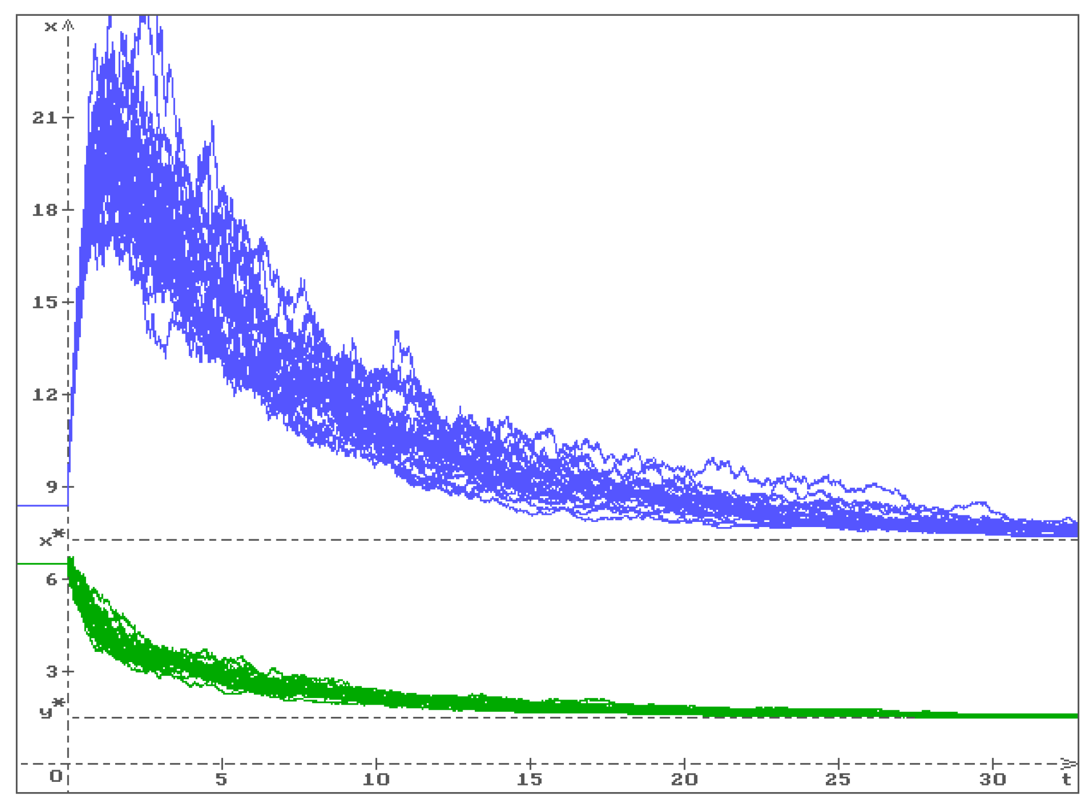
In Figure 1, 25 trajectories (blue) and (green) of the solution of system (7) and (8) are presented by the values of the parameters (26) with the initial conditions , , . The equilibrium is stable in probability, so all trajectories converge to this equilibrium.
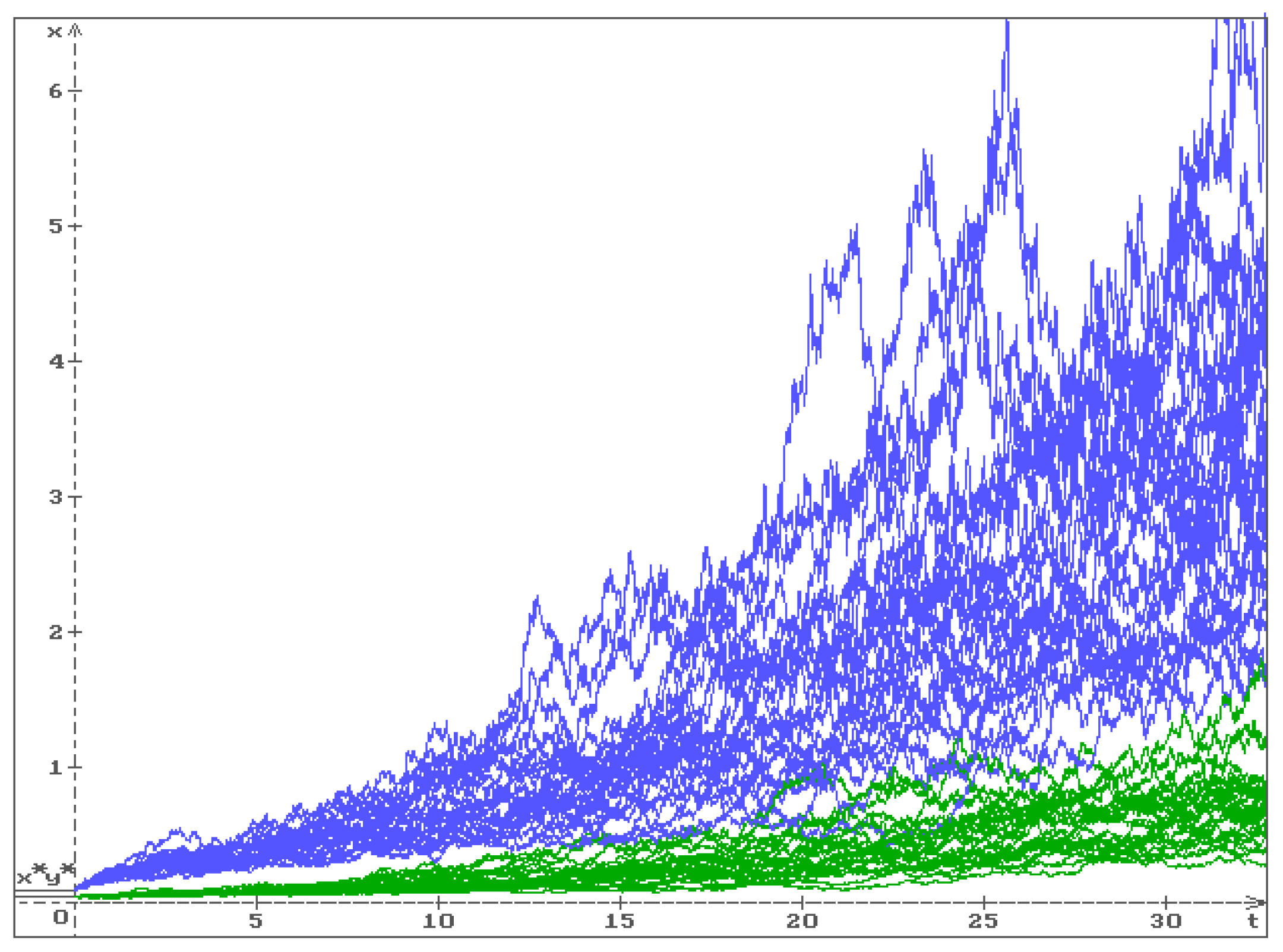
In Figure 2, 25 trajectories (blue) and (green) of the solution of system (7) and (8) are presented by the values of the parameters (26) with the initial conditions , , . The equilibrium is unstable, and all trajectories go out of this equilibrium.
Example 2.
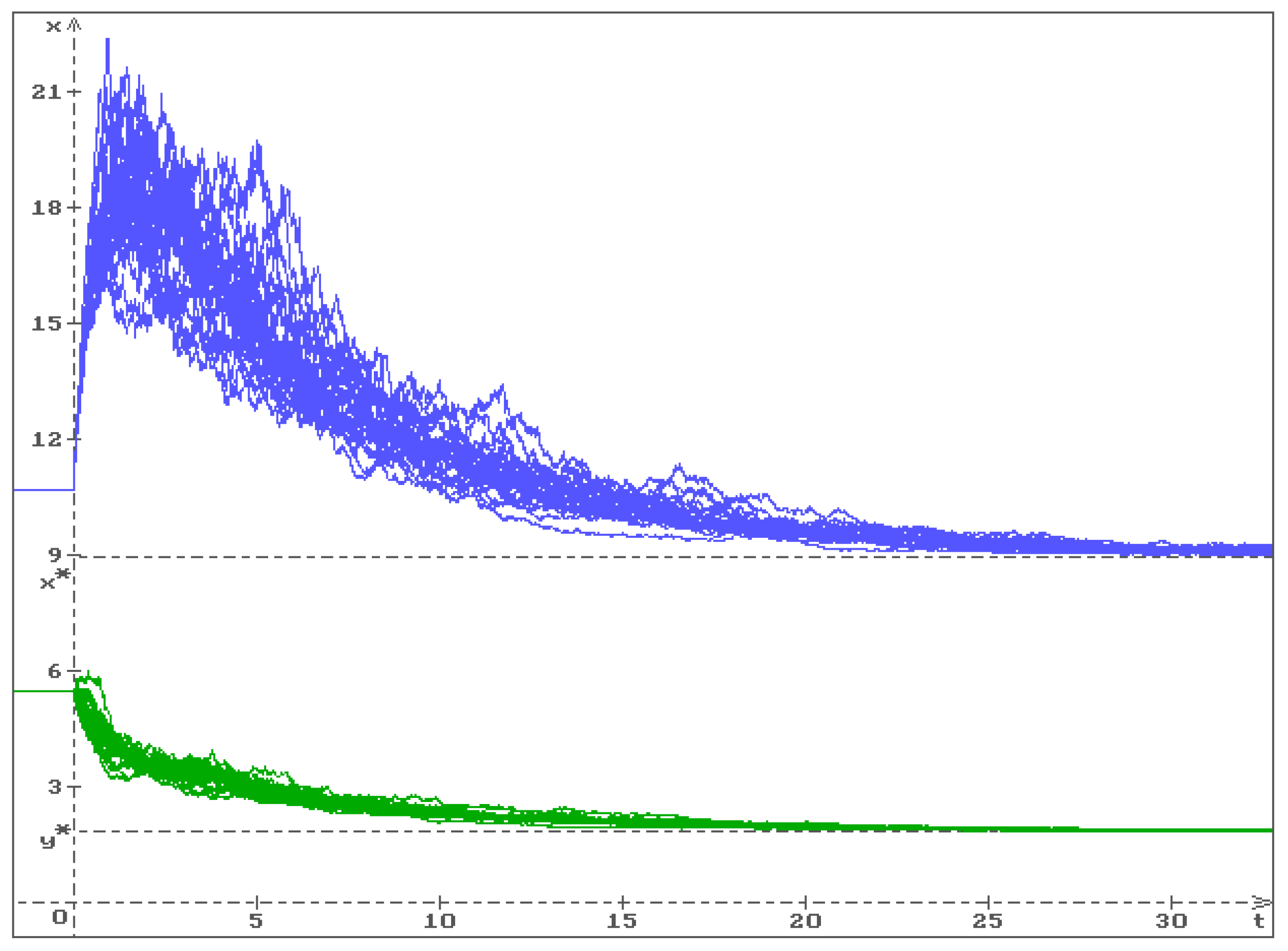
In Figure 3, 25 trajectories (blue) and (green) of the solution of system (7) and (8) are presented by the values of the parameters (26) with the initial conditions , , . The equilibrium is stable in probability, so all trajectories converge to this equilibrium.
4. Conclusions
It is shown how the Lyapunov functionals construction method and the method of linear matrix inequalities (LMIs) can be used for stability and instability investigation of nonlinear systems with a state-dependent delay under stochastic perturbations. Obtained delay-independent and delay-dependent conditions of stability in probability for equilibria of the considered system are formulated in terms of linear matrix inequalities and are illustrated by numerical simulation of solutions of Ito’s stochastic differential equation. The proposed method of stability investigation can be successfully used for similar investigations of other types of nonlinear systems with state-dependent delay under stochastic perturbations.
Funding
This research received no external funding.
Data Availability Statement
Not applicable.
Conflicts of Interest
The author declares no conflict of interest.
Appendix A. Lyapunov Type Theorems
Consider Ito’s stochastic differential equation of neutral type [14,17,18].
where is a value of the solution of Equation (A1) in the time moment t, , , is the trajectory of the solution of Equation (A1) until the time moment t, is a space of -adapted functions , , with continuous trajectories and norm .
Consider a functional that can be presented in the form , , and for put
Denote by D the set of the functionals, for which the function defined in (A2) has a continuous derivative with respect to t and two continuous derivatives with respect to x. Let ∇ and be respectively the first and the second derivatives of the function with respect to x. For the functionals from D the generator L of Equation (A1) has the form [14,15]
Theorem A1
([14]). Let and there exist a functional , positive constants , , , such that the following conditions hold:
References
- Akhtari, B. Numerical solution of stochastic state-dependent delay differential equations: Convergence and stability. Adv. Differ. Equ. 2019, 396, 34. [Google Scholar] [CrossRef] [Green Version]
- Arthi, G.; Park, J.H.; Jung, H.Y. Existence and controllability results for second-order impulsive stochastic evolution systems with state-dependent delay. Appl. Math. Comput. 2014, 248, 328–341. [Google Scholar] [CrossRef]
- Kazmerchuk, Y.I.; Wu, J.H. Stochastic state-dependent delay differential equations with applications in finance. Funct. Differ. Equations 2004, 11, 77–86. [Google Scholar]
- Parthasarathy, C.; Arjunan, M.M. Controllability results for first order impulsive stochastic functional differential systems with state-dependent delay. J. Math. Comput. Sci. 2013, 3, 15–40. [Google Scholar]
- Zuomao, Y.; Lu, F. Existence and controllability of fractional stochastic neutral functional integro-differential systems with state-dependent delay in Frechet spaces. J. Nonlinear Sci. Appl. 2016, 9, 603–616. [Google Scholar]
- Zuomao, Y.; Zhang, H. Existence of solutions to impulsive fractional partial neutral stochastic integro-differential inclusions with state-dependent delay. Electron. J. Differ. Equ. 2013, 81, 1–21. [Google Scholar]
- Cooke, K.L.; Huang, W. On the problem of linearization for state-dependent delay differential equations. Proc. Am. Math. Soc. 1996, 124, 1417–1426. [Google Scholar] [CrossRef]
- Wang, Y.; Liu, X.; Wei, Y. Dynamics of a stage-structured single population model with state-dependent delay. Adv. Differ. Equ. 2018, 2018, 364. [Google Scholar] [CrossRef] [Green Version]
- Shaikhet, L. Stability of stochastic differential equation with distributed and state-dependent delays. J. Appl. Math. Comput. 2020, 4, 181–188. [Google Scholar] [CrossRef]
- Shaikhet, L. About one method of stability investigation for nonlinear stochastic delay differential equations. Int. J. Robust Nonlinear Control 2021, 31, 2946–2959. [Google Scholar] [CrossRef]
- Shaikhet, L. Some generalization of the method of stability investigation for nonlinear stochastic delay differential equations. Symmetry 2022, 14, 1734. [Google Scholar] [CrossRef]
- Fridman, E.; Shaikhet, L. Stabilization by using artificial delays: An LMI approach. Automatica 2017, 81, 429–437. [Google Scholar] [CrossRef]
- Fridman, E.; Shaikhet, L. Simple LMIs for stability of stochastic systems with delay term given by Stieltjes integral or with stabilizing delay. Syst. Control. Lett. 2019, 124, 83–91. [Google Scholar] [CrossRef]
- Shaikhet, L. Lyapunov Functionals and Stability of Stochastic Functional Differential Equations; Springer Science & Business Media: Berlin/Heidelberg, Germany, 2013. [Google Scholar]
- Gikhman, I.I.; Skorokhod, A.V. Stochastic Differential Equations; Springer: Berlin/Heidelberg, Germany, 1972. [Google Scholar]
- Beretta, E.; Kolmanovskii, V.; Shaikhet, L. Stability of epidemic model with time delays influenced by stochastic perturbations. Math. Comput. Simul. 1998, 45, 269–277. [Google Scholar] [CrossRef]
- Kolmanovskii, V.B.; Myshkis, A.D. Introduction to the Theory and Applications of Functional Differential Equations; Kluwer Academic: Dordrecht, The Netherlands, 1999. [Google Scholar]
- Kolmanovskii, V.B.; Nosov, V.R. Stability of Functional Differential Equations; Academic Press: London, UK, 1986. [Google Scholar]
- Melchor-Aguilar, D.; Kharitonov, V.I.; Lozano, R. Stability conditions for integral delay systems. Int. J. Robust Nonlinear Control 2010, 20, 1–15. [Google Scholar] [CrossRef]
Figure 1.
Stable equilibrium : 25 trajectories (blue) and (green) for , , , , , , , and the initial conditions , , . One can see that all trajectories converge to the equilibrium .
Figure 1.
Stable equilibrium : 25 trajectories (blue) and (green) for , , , , , , , and the initial conditions , , . One can see that all trajectories converge to the equilibrium .

Figure 2.
Unstable equilibrium : 25 trajectories (blue) and (green) for , , , , , , , and the initial conditions , , . One can see that all trajectories go out of the equilibrium .
Figure 2.
Unstable equilibrium : 25 trajectories (blue) and (green) for , , , , , , , and the initial conditions , , . One can see that all trajectories go out of the equilibrium .

Figure 3.
Stable equilibrium : 25 trajectories (blue) and (green) for , , , , , , and the initial conditions , , . One can see that all trajectories converge to the equilibrium .
Figure 3.
Stable equilibrium : 25 trajectories (blue) and (green) for , , , , , , and the initial conditions , , . One can see that all trajectories converge to the equilibrium .

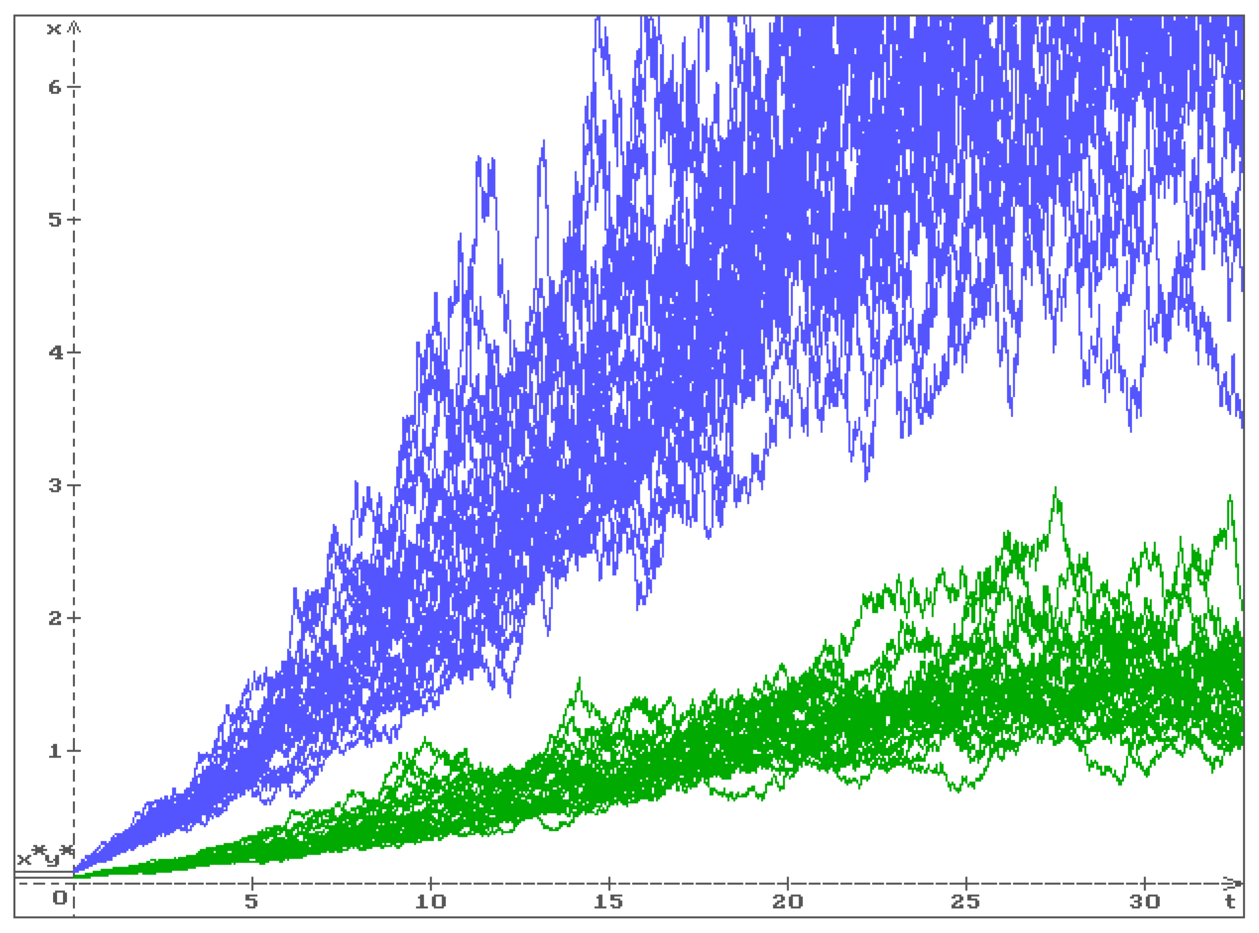
Figure 4.
Unstable equilibrium : 25 trajectories (blue) and (green) for , , , , , , and the initial conditions , , . One can see that all trajectories go out of the equilibrium .
Figure 4.
Unstable equilibrium : 25 trajectories (blue) and (green) for , , , , , , and the initial conditions , , . One can see that all trajectories go out of the equilibrium .

Publisher’s Note: MDPI stays neutral with regard to jurisdictional claims in published maps and institutional affiliations. |
© 2022 by the author. Licensee MDPI, Basel, Switzerland. This article is an open access article distributed under the terms and conditions of the Creative Commons Attribution (CC BY) license (https://creativecommons.org/licenses/by/4.0/).
Share and Cite
MDPI and ACS Style
Shaikhet, L. About Stability of Nonlinear Stochastic Differential Equations with State-Dependent Delay. Symmetry 2022, 14, 2307. https://doi.org/10.3390/sym14112307
AMA Style
Shaikhet L. About Stability of Nonlinear Stochastic Differential Equations with State-Dependent Delay. Symmetry. 2022; 14(11):2307. https://doi.org/10.3390/sym14112307
Chicago/Turabian StyleShaikhet, Leonid. 2022. "About Stability of Nonlinear Stochastic Differential Equations with State-Dependent Delay" Symmetry 14, no. 11: 2307. https://doi.org/10.3390/sym14112307
Note that from the first issue of 2016, this journal uses article numbers instead of page numbers. See further details here.