Article

An Optimization Approach with Single-Valued Neutrosophic Hesitant Fuzzy Dombi Aggregation Operators

1
Department of mathematics, University of the Punjab, Lahore 54590, Pakistan
2
Mathematics, Physical and Natural Sciences Division, University of New Mexico, Gallup Campus, Gallup, NM 87301, USA
3
Department of Operations Research and Statistics, Faculty of Organizational Sciences, University of Belgrade, 11000 Belgrade, Serbia
4
The Faculty of Civil Aviation, Megatrend University, 11000 Belgrade, Serbia
*
Author to whom correspondence should be addressed.
Symmetry 2022, 14(11), 2271; https://doi.org/10.3390/sym14112271
Submission received: 8 October 2022 / Revised: 21 October 2022 / Accepted: 26 October 2022 / Published: 29 October 2022
(This article belongs to the Special Issue Recent Advances in Fuzzy Optimization Methods and Models)

Abstract

:
Using the strength of a single-valued neutrosophic set (SVNS) with the flexibility of a hesitant fuzzy set (HFS) yields a robust model named the single-valued neutrosophic hesitant fuzzy set (SVNHFS). Due to the ability to utilize three independent indexes (truthness, indeterminacy, and falsity), an SVNHFS is an efficient model for optimization and computational intelligence (CI) as well as an intelligent decision support system (IDSS). Taking advantage of the flexibility of operational parameters in Dombi’s t-norm and t-conorm operations, new aggregation operators (AOs) are proposed, which are named the SVN fuzzy Dombi weighted averaging (SVNHFDWA) operator, SVN hesitant fuzzy Dombi ordered weighted averaging (SVNHFDOWA) operator, SVN hesitant fuzzy Dombi hybrid averaging (SVNHFDHWA) operator, SVN hesitant fuzzy Dombi weighted geometric (SVNHFDWG) operator, SVN hesitant fuzzy Dombi ordered weighted geometric (SVNHFDOWG) operator as well as SVN hesitant fuzzy Dombi hybrid weighted geometric (SVNHFDHWG) operator. The efficiency of these AOs is investigated in order to determine the best option using SVN hesitant fuzzy numbers (SVNHFNs) in an IDSS. Additionally, a practical application of SVNHFDWA and SVNHFDWG is also presented to examine symmetrical analysis in the selection of wireless charging station for vehicles.
MSC:
03E72; 94D05; 90B50

1. Introduction

The researchers have struggled for centuries to comprehend the complex relationship between precision and ambiguity. Zadeh [1] was attempting to solve the problem of dealing with uncertain and imprecise information in the framework of computational intelligence when the novel notion of a fuzzy set (FS) developed. In this framework, each object’s membership degree (MD) is composed of a single value which lies in [ 0 , 1 ] . One of its disadvantages is that it only supports MD and does not allow non-membership degree (NMD) to be expressed. Atanassov [2] invented an intuitionistic fuzzy set (IFS) to circumvent the constraints imposed by FS. The MD and NMD of an IFS, both of which have values from 0 and 1, can be used to evaluate the structure of objects. A wide range of information aggregation have been developed in order to consolidate knowledge that is intuitively ambiguous. These aggregation methods have been created to make the information more reasonable and accurate.
Xu [3] was responsible for the creation of multiple kinds of aggregation operators (AOs), including IF weighted, and other operators. Xu is [3] credited with the invention of multiple types of averaging operators, including the IF weighted, ordered weighted, and hybrid averaging operators, amongst other types of averaging operators. These operators are still very useful today. An interval-valued intuitionistic fuzzy set (IVIFS) was presented in [4] as a further developments of an IFS, which is defined by its interval MF and interval NMF in [ 0 , 1 ] .
The authors in [4] suggested the further aspects of an interval-valued intuitionistic fuzzy set (IVIFS), which is distinguished by MD and NMD as fuzzy intervals. This was completed in an effort to further generalize IFSs. Since IFSs and IVIFSs cannot effectively describe uncertain and vague data, Smarandache [5] designed a neutrosophic set (NS) from a mathematical perspective as a technique of expressing imprecise information. The study of an SVNS [6] is more realistic due to its components in compact set [ 0 , 1 ] . An interval neutrosophic set (INS) [7] is another interesting extension of the NS model. A hesitant fuzzy set [8,9] has the ability to seek a solution to the problem of determining the extent to which an individual component belongs to a set, which is notoriously difficult to do. HFS can be seen as a suitable way of permitting multiple different degrees for an element to be added to a set, which is suitable for addressing hesitancy, which is the most prevalent difficulty that arises while making decisions. Because of the circumstance that there is just few truth-membership hesitant grades in an HFS, the challenge cannot be characterized utilizing truth-MD, indeterminacy, or falsity-MD. This is due to the hesitation of decision makers to make suitable choices. On the other hand, an SVNS enables a chance and opportunity to capture vague knowledge that arises from the real-world circumstances. It is quite preferable to handle information that is vague as well as uncertain if possible. It is very useful to describe the degree of truth-MD, indeterminacy, and falsity-MD for IDSS and CI. In order to deal with this scenario, Ye [10] was the one who gave the idea of the SVN hesitant fuzzy set.
One perspective on decision making describes it as a process of problem solving that culminates in the selection of a solution that is considered to be either the optimal or at least an acceptable and reasonable alternative among a set of feasible alternatives. MCDM, which stands for multi-criteria decision making, is a branch of operations research that focuses on the method of determining the best option for a specific set of criteria by thoroughly and rigorously analyzing all of the options that are available. This is accomplished by comparing and contrasting all of the potential choices.
On a continual basis, MCDM challenges and their associated solutions are confronted in multiple fields including the social sciences, economics, management, and medicine. Among the most complex obstacles that one faces when encountering complexities that require MCDM is scrambling to figure out how to incorporate uncertain information pieces that have been provided by a diverse range of sources in the process of arriving at a judgement or conclusions. This is one of the most significant challenges that one faces when encountering challenges that require MCDM.
Researchers utilized a variety of methods, such as rules, aggregation-specific procedures, and various extensions of FS theory, in order to obtain an outstanding aggregation. All of these methodologies are founded on various quantitative aggregation operations. The aggregation operators are remarkably beneficial tools to use when it involves the process of consolidating a variety of information into a single information. A substantial amount of study is currently being directed into comprehending the information aggregation techniques, which are an important tool in their own right. Ye [10] proposed SVNHF averaging operator and SVNHF geometric operator (SVNHFWG). In [11] SVNHF ordered weighted averging (SVNHFOWA) operator and SVNHF hybrid averaging (SVNHFHA) operator were studied. Both The Dombi t-norm and the t-conorm operations, which show how essential it is to have a high degree of flexibility with regard to the operational parameter, were hypothesized of and produced by Dombi [12]. Some operators for IFS, IVIFS, PFS, SVNS, HFS and SVNHFSs are listed in Table 1.
Hanif et al. [46] developed linear Diophontine fuzzy (LDF) graphs with a fresh take on how decisions are made in regard to medical diagnosis. Prakash et al. [47] came up with the innovative ideas of LDF-graph and examined the elements of extending the lifespan of a wireless charging network by employing a mobile robot. Mohamed et al. [48] He developed a study on the assessment of the autonomous charger for electric vehicles (EV) and hybrid electric vehicles (HEV). Tang et al. [49] proposed a symmetric implicational algorithm derived from the intuitionistic fuzzy entropy method. Wang [50] proposed a robust intuitionistic fuzzy analytic hierarchy process. Fuzzy optimization techniques have been utilized by various researchers [51,52,53,54,55,56,57,58]. Shi and Ye [59] proposed Dombi AO for aggregation of neutrosophic cubic sets.
This article provides a number of aggregation operators for the SVNHF framework. Some key features are also demonstrated, including idempotency, monotonicity, boundedness, and commutativity. In addition, a technique for handling IDSS problems is given by utilizing the SVNHFDWA operator and SVNHFDWG operator. In IDSS, an application of SVNHFDWA operator and SVNHFDWG operator is provided. A practical application of SVNHFDWA and SVNHFDWG is also presented to examine symmetrical analysis in the selection of a feasible mobile robot (mobile charger) for electric vehicles (EV) as well as hybrid electric vehicles (HEV).
In Section 2, we review NS, SVNS, HFS, SVNHFS, and their fundamental operations. In Section 3, we study some operational laws of SVNHFSs, and a series of robust AOs are developed in Section 4 that include SVNHFDWA, SVNHFDWG, SVNHFDOWA, SVNHFDOWG, SVNHFDHWA, and SVNHFDHWG. In Section 5, an illustration is established to utilize SVNHFDWA and SVNHFDWG that are helpful in IDSS that might be applied in real-world situations particularly in the selection of feasible mobile robots (mobile charger).

2. Preliminaries

Definition 1 
([5]). Let X be any set. A neutrosophic set (NS) A in X can be identified by the mappings T A , I A , N A : X ( 0 , 1 + ) such that 0 sup T A ( x ) + sup I A ( x ) + sup N A ( x ) 3 + , x X .
Example 1. 
Let X = { ρ 1 , ρ 2 , ρ 3 , ρ 4 , ρ 5 } be a universal set. Then, the NS will be
A = { ρ 1 , { 0.325 , 0.746 , 0.267 } , ρ 2 , { 0.313 , 0.435 , 0.918 } , ρ 3 , { 0.142 , 0.278 , 0.538 } , ρ 4 , { 0.434 , 0.787 , 0.167 } , ρ 5 , { 0.934 , 0.487 , 0.067 } }
Definition 2 
([6]). An SVN S in X is identified by truth-MD T S ( x ) , indeterminacy I S ( x ) , and falsity-MD N S ( x ) such that for each point x in X , T S ( x ) , I S ( x ) , N S ( x ) [ 0 , 1 ] as well as 0 T S ( x ) + I S ( x ) + N S ( x ) 3 . Then, an SVNS S becomes of the form
S = { x , T S ( x ) , I S ( x ) , N S ( x ) | x X }
Definition 3 
([9]). An HFS H in X associates a finite subset of [ 0 , 1 ] to each object ς X . It can be expressed as
H = { ς , h ( ς ) ς X } .
Example 2. 
Let X = { x 1 , x 2 , x 3 , x 4 , x 5 } be a set. Then, the HFS will be
H = { x 1 , { 0.125 , 0.3450 . 867 } , x 2 , { 0.333 , 0.445 , 0.509 , 0.689 } , x 3 , { 0.378 , 0.432 } , x 4 , { 0.004 , 0.243 , 0.754 } , x 5 , { 0.669 , 0.775 } }
where
h ( x 1 ) = { 0.125 , 0.3450 . 867 }
h ( x 2 ) = { 0.333 , 0.445 , 0.509 , 0.689 }
h ( x 3 ) = { 0.378 , 0.432 }
h ( x 4 ) = { 0.004 , 0.243 , 0.754 }
h ( x 5 ) = { 0.669 , 0.775 }
are HF-elements corresponding to x 1 , x 2 , x 3 , x 4 and x 5 , respectively.
Definition 4 
([10]). Let X be a universal set; an SVNHFS in X is expressed as
T = { x , P ( x ) , I ( x ) , N ( x ) | x X }
such that the possible truth-membership hesitant degrees (THD) are represented by P ( x ) , indeterminacy-membership hesitant degrees (IHD) are represented by I ( x ) , and falsity-membership hesitant degrees (FHD) are represented by N ( x ) , respectively.
Example 3. 
Let X = { x 1 , x 2 , x 3 , x 4 } be a universal set. Then, the SVNHFS will be
T = { x 1 , { 0.645 , 0.125 , 0.667 } , { 0.211 } , { 0.111 , 0.200 } , x 2 , { 0.133 , 0.345 } , { 0.988 , 0.259 } , { 0.335 , 0.121 } , x 3 , { 0.511 } , { 0.124 , 0.654 } , { 0.652 , 0.783 , 0.284 } , x 4 , { 0.481 , 0.872 , 0.100 , 0.321 } , { 0.865 } , { 0.768 } }
Definition 5 
([10]). If x 1 = P 1 ( x ) , I 1 ( x ) , N 1 ( x ) , x 2 = P 2 ( x ) , I 2 ( x ) , N 2 ( x ) are two SNVHFNs in X, then
(i) 
x 1 c = { N 1 ( x ) , 1 I 1 ( x ) , P 1 ( x ) }
(ii) 
x 1 x 2 P 1 ( x ) P 2 ( x ) , I 1 ( x ) I 2 ( x ) and N 1 ( x ) N 2 ( x ) for any x N .
(iii) 
x 1 x 2 = P ( P 1 P 2 ) | P max ( P 1 P 2 ) , I ( I 1 I 2 ) | I min ( I 1 + I 2 + ) , N ( N 1 N 2 ) | N min ( N 1 + N 2 + )
(iv) 
x 1 x 2 = P ( P 1 P 2 ) | P min ( P 1 + P 2 + ) , I ( I 1 I 2 ) | I max ( I 1 I 2 ) , N ( N 1 N 2 ) | N max ( N 1 N 2 )
(v) 
x 1 x 2 = { P 1 P 2 , I 1 I 2 , N 1 N 2 } = ϕ 1 P 1 φ 1 I 1 ψ 1 N 1 ϕ 2 P 2 φ 2 I 2 ψ 2 N 2 { ϕ 1 + ϕ 2 ϕ 1 ϕ 2 } , { φ 1 φ 2 } , { ψ 1 ψ 2 }
(vi) 
x 1 x 2 = { P 1 P 2 , I 1 I 2 , N 1 N 2 } = ϕ 1 P 1 φ 1 I 1 ψ 1 N 1 ϕ 2 P 2 φ 2 I 2 ψ 2 N 2 { ϕ 1 ϕ 2 } , { φ 1 + φ 2 φ 1 φ 2 } , { ψ 1 + ψ 2 ψ 1 ψ 2 }
(vii) 
θ x 1 = ϕ 1 P 1 φ 1 I 1 ψ 1 N 1 { 1 ( 1 ϕ 1 ) θ } , { φ 1 ) θ } , { ψ 1 θ } , θ > 0
(viii) 
x 1 θ = ϕ 1 P 1 φ 1 I 1 ψ 1 N 1 { ( ϕ 1 ) θ } , { 1 ( 1 φ 1 ) θ } , { 1 ( 1 ψ 1 ) θ } , θ > 0
Definition 6 
([60]). Let x = P , I , N be a SVNHFN. The score function S ( x ) of x becomes
S ( x ) = 1 3 2 + 1 l P ϕ P ϕ 1 l I φ I φ 1 l N ψ N ψ
Definition 7 
([60]). Let x = P , I , N be a SVNHFN. The accuracy function A ( x ) of x becomes
A ( x ) = 1 l P ϕ P ϕ 1 l N ψ N ψ
Definition 8 
([60]). Let x = P , I , N be a SVNHFN. The certain function C ( x ) of x becomes
C ( x ) = 1 l P ϕ P ϕ
Let x 1 and x 2 be two SVNHFNs. Then:
  • As S ( x 1 ) > S ( x 2 ) , then x 1 is superior to x 2 , designated by x 1 x 2
  • As S ( x 1 ) = S ( x 2 ) and A ( x 1 ) > A ( x 2 ) , then x 1 is superior to x 2 , which is designated by x 1 x 2 .
  • As S ( x 1 ) = S ( x 2 ) , A ( x 1 ) = A ( x 2 ) and C ( x 1 ) > C ( x 2 ) , then x 1 is superior to x 2 , which is designated by x 1 x 2
  • As S ( x 1 ) = S ( x 2 ) , A ( x 1 ) = A ( x 2 ) and C ( x 1 ) = C ( x 2 ) , then x 1 is equal to x 2 , which is designated by x 1 x 2
Definition 9 
([12]). Consider a and b any two real numbers. Dombi t-norm and Dombi t-conorm can be elaborated as follows.
Dom ( a , b ) = 1 1 + 1 a a λ + 1 b b λ 1 / λ
Dom c ( a , b ) = 1 1 1 + a 1 a λ + b 1 b λ 1 / λ
where λ 1 and ( a , b ) [ 0 , 1 ] 2 .

3. Dombi Operations for SVNHFNs

Let x 1 = P 1 ( x ) , I 1 ( x ) , N 1 ( x ) , x 2 = P 2 ( x ) , I 2 ( x ) , N 2 ( x ) and x = P ( x ) , I ( x ) , N ( x ) be three SNVHFNs in X; then, the Dombi operations can be defined as:
  • x 1 x 2 = ϕ 1 P 1 , ϕ 2 P 2 , φ 1 I 1 , φ 2 I 2 , ψ 1 N 1 , ψ 2 N 2 1 1 1 + ϕ 1 1 ϕ 1 λ + ϕ 2 1 ϕ 2 λ 1 / λ , 1 1 + 1 φ 1 φ 1 λ + 1 φ 2 φ 2 λ 1 / λ , 1 1 + 1 ψ 1 ψ 1 λ + 1 ψ 2 ψ 2 λ 1 / λ
  • x 1 x 2 = ϕ 1 P 1 , ϕ 2 P 2 , φ 1 I 1 , φ 2 I 2 , ψ 1 N 1 , ψ 2 N 2 1 1 + 1 ϕ 1 ϕ 1 λ + 1 ϕ 2 ϕ 2 λ 1 / λ , 1 1 1 + φ 1 1 φ 1 λ + φ 2 1 φ 2 λ 1 / λ , 1 1 1 + ψ 1 1 ψ 1 λ + ψ 2 1 ψ 2 λ 1 / λ ,
  • ρ x = ϕ P , φ I , ψ N 1 1 1 + ρ ϕ 1 ϕ λ 1 / λ , 1 1 + ρ 1 φ φ λ 1 / λ , 1 1 + ρ 1 ψ ψ λ 1 / λ
  • x ρ = ϕ P , φ I , ψ N 1 1 + ρ 1 ϕ ϕ λ 1 / λ , 1 1 1 + ρ φ 1 φ λ 1 / λ , 1 1 1 + ρ ψ 1 ψ λ 1 / λ
Theorem 1. 
Let x 1 = P 1 ( x ) , I 1 ( x ) , N 1 ( x ) and x 2 = P 2 ( x ) , I 2 ( x ) , N 2 ( x ) be two SVNHFNs and ρ , ρ 1 , ρ 2 0 be any real numbers; then,
(i) 
x 1 x 2 = x 2 x 1 .
(ii)  
x 1 x 2 = x 2 x 1 .
(iii) 
( x 1 x 2 ) ρ = x 1 ρ x 2 ρ .
(iv) 
ρ ( x 1 x 2 ) = ρ x 1 ρ x 2 .
(v) 
x 1 ρ 1 x 1 ρ 2 = x 1 ρ 1 + ρ 2 .
(vi) 
ρ 1 ( ρ 2 x 1 ) = ( ρ 1 ρ 2 ) x 1 .
(vii) 
( x 1 ρ 1 ) ρ 2 = ( x 1 ) ρ 1 ρ 2 .
(viii) 
ρ 1 x 1 ρ 2 = ( ρ 1 + ρ 2 ) x 1 .
(ix) 
x 1 c x 2 c = ( x 1 x 2 ) c .
(x) 
x 1 c x 2 c = ( x 1 x 2 ) c .
Proof. 
Proof is straight forward.    □

4. Dombi Operators for SVNHF Information

Now, we look at the Dombi SVNHF aggregation operators using SVNHF Dombi operations which are discussed in the previous section. This section introduces a number of aggregation operators, including the SVNHFDWA, SVNHFDWG, SVNHFDOWA, SVNHFDOWG, SVNHFDHA, SVNHFDHG.

4.1. SVNHFDWA Operator

Definition 10. 
Consider a collection of SVNHFNs x i ( i = 1 , 2 , , n ) ; then, the SVNHFDWA operator is defined as follows:
S V N H F D W A ( x 1 , x 2 , , x n ) = i = 1 n ( w i x i ) = w 1 x 1 w 2 x 2 w n x n
Equation (6) gives w = ( w 1 , w 2 , , w n ) T , which is a weight vector (WV) of the SVNHFNs x i ( i = 1 , 2 , , n ) , w i [ 0 , 1 ] with i = 1 n w i = 1 .
Theorem 2. 
Consider a collection of SVNHFNs x i ( i = 1 , 2 , , n ) with WVs w = ( w 1 , w 2 , , w n ) T ; then, the aggregated SVNHFN is SVNHFDWA ( x 1 , x 2 , , x n ) = i = 1 n ( w i x i ) = ϕ 1 P 1 , ϕ 2 P 2 , , ϕ n P n , φ 1 I 1 , φ 2 I 2 , , φ n I n , ψ 1 N 1 , ψ 2 N 2 , , ψ n N n   
1 1 1 + i = 1 n w i ϕ i 1 ϕ i λ 1 / λ , 1 1 + i = 1 n w i 1 φ i φ i λ 1 / λ , 1 1 + i = 1 n w i 1 ψ i ψ i λ 1 / λ
Proof. 
Equation (7) can be proved by using induction on n:
For n = 2 , as
w 1 x 1 = ϕ 1 P 1 , φ 1 I 1 , ψ 1 N 1 1 1 1 + w 1 ϕ 1 1 ϕ 1 λ 1 / λ , 1 1 + w 1 1 φ 1 φ 1 λ 1 / λ , 1 1 + w 1 1 ψ 1 ψ 1 λ 1 / λ
w 2 x 2 = ϕ 2 P 2 , φ 2 I 2 , ψ 2 N 2 1 1 1 + w 2 ϕ 2 1 ϕ 2 λ 1 / λ , 1 1 + w 2 1 φ 2 φ 2 λ 1 / λ , 1 1 + w 2 1 ψ 2 ψ 2 λ 1 / λ then, taking union for ϕ 1 P 1 , ϕ 2 P 2 , φ 1 I 1 , φ 2 I 2 , ψ 1 N 1 , ψ 2 N 2
w 1 x 1 w 2 x 2 = { 1 1 1 + 1 1 1 + w 1 ϕ 1 1 ϕ 1 λ 1 / λ 1 1 + 1 1 + w 1 ϕ 1 1 ϕ 1 λ 1 / λ λ + 1 1 1 + w 2 ϕ 2 1 ϕ 2 λ 1 / λ 1 1 + 1 1 + w 2 ϕ 2 1 ϕ 2 λ 1 / λ λ 1 / λ ,
1 1 + 1 1 1 + w 1 1 φ 1 φ 1 λ 1 / λ 1 1 + w 1 1 φ 1 φ 1 λ 1 / λ λ + 1 1 1 + w 2 1 φ 2 φ 2 λ 1 / λ 1 1 + w 2 1 φ 2 φ 2 λ 1 / λ λ 1 / λ ,
1 1 + 1 1 1 + w 1 1 ψ 1 ψ 1 λ 1 / λ 1 1 + w 1 1 ψ 1 ψ 1 λ 1 / λ λ + 1 1 1 + w 2 1 ψ 2 ψ 2 λ 1 / λ 1 1 + w 2 1 ψ 2 ψ 2 λ 1 / λ λ 1 / λ }
= { 1 1 1 + 1 + w 1 ϕ 1 1 ϕ 1 λ 1 / λ 1 1 + w 1 ϕ 1 1 ϕ 1 λ 1 / λ 1 1 + w 1 ϕ 1 1 ϕ 1 λ 1 / λ λ + 1 + w 2 ϕ 2 1 ϕ 2 λ 1 / λ 1 1 + w 2 ϕ 2 1 ϕ 2 λ 1 / λ 1 1 + w 2 ϕ 2 1 ϕ 2 λ 1 / λ λ 1 / λ ,
1 1 + 1 + w 1 1 φ 1 φ 1 λ 1 / λ 1 1 + w 1 1 φ 1 φ 1 λ 1 / λ 1 1 + w 1 1 φ 1 φ 1 λ 1 / λ λ + 1 + w 2 1 φ 2 φ 2 λ 1 / λ 1 1 + w 2 1 φ 2 φ 2 λ 1 / λ 1 1 + w 2 1 φ 2 φ 2 λ 1 / λ λ 1 / λ ,
1 1 + 1 + w 1 1 ψ 1 ψ 1 λ 1 / λ 1 1 + w 1 1 ψ 1 ψ 1 λ 1 / λ 1 1 + w 1 1 ψ 1 ψ 1 λ 1 / λ λ + 1 + w 2 1 ψ 2 ψ 2 λ 1 / λ 1 1 + w 2 1 ψ 2 ψ 2 λ 1 / λ 1 1 + w 2 1 ψ 2 ψ 2 λ 1 / λ λ 1 / λ }
= ϕ 1 P 1 , ϕ 2 P 2 , φ 1 I 1 , φ 2 I 2 , ψ 1 N 1 , ψ 2 N 2 1 1 1 + w 1 ϕ 1 1 ϕ 1 λ + w 2 ϕ 2 1 ϕ 2 λ 1 / λ , 1 1 + w 1 1 φ 1 φ 1 λ + w 2 1 φ 2 φ 2 λ 1 / λ , 1 1 + w 1 1 ψ 1 ψ 1 λ + w 2 1 ψ 2 ψ 2 λ 1 / λ As Equation (7) is satisfied for n = k , that is
i = 1 k ( w i x i ) = ϕ 1 P 1 , ϕ 2 P 2 , , ϕ k P k , φ 1 I 1 , φ 2 I 2 , , φ k I k , ψ 1 N 1 , ψ 2 N 2 , , ψ k N k 1 1 1 + i = 1 k w i ϕ i 1 ϕ i λ 1 / λ , 1 1 + i = 1 k w i 1 φ i φ i λ 1 / λ , 1 1 + i = 1 k w i 1 ψ i ψ i λ 1 / λ then, when n = k + 1 , by the Dombi addition operation, we have
i = 1 k + 1 ( w i x i ) = i = 1 k ( w i x i ) ( w k + 1 x k + 1 ) = ϕ 1 P 1 , ϕ 2 P 2 , , ϕ k P k , φ 1 I 1 , φ 2 I 2 , , φ k I k , ψ 1 N 1 , ψ 2 N 2 , , ψ k N k 1 1 1 + i = 1 k w i ϕ i 1 ϕ i λ 1 / λ , 1 1 + i = 1 k w i 1 φ i φ i λ 1 / λ , 1 1 + i = 1 k w i 1 ψ i ψ i λ 1 / λ ϕ k + 1 P k + 1 , φ k + 1 I k + 1 , ψ k + 1 N k + 1 1 1 1 + w k + 1 ϕ k + 1 1 ϕ k + 1 λ 1 / λ , 1 1 + w k + 1 1 φ k + 1 φ k + 1 λ 1 / λ , 1 1 + w k + 1 1 ψ k + 1 ψ k + 1 λ 1 / λ
= ϕ 1 P 1 , ϕ 2 P 2 , , ϕ k + 1 P k + 1 , φ 1 I 1 , φ 2 I 2 , , φ k + 1 I k + 1 , ψ 1 N 1 , ψ 2 N 2 , , ψ k + 1 N k + 1 1 1 1 + i = 1 k + 1 w i ϕ i 1 ϕ i λ 1 / λ , 1 1 + i = 1 k + 1 w i 1 φ i φ i λ 1 / λ , 1 1 + i = 1 k + 1 w i 1 ψ i ψ i λ 1 / λ i.e., Equation (7) is satisfied for n = k + 1 . Thus, Equation (7) is satisfied for all n. Then,
SVNHFDWA ( x 1 , x 2 , , x n ) = i = 1 n ( w i x i ) = ϕ 1 P 1 , ϕ 2 P 2 , , ϕ n P n , φ 1 I 1 , φ 2 I 2 , , φ n I n , ψ 1 N 1 , ψ 2 N 2 , , ψ n N n 1 1 1 + i = 1 n w i ϕ i 1 ϕ i λ 1 / λ , 1 1 + i = 1 n w i 1 φ i φ i λ 1 / λ , 1 1 + i = 1 n w i 1 ψ i ψ i λ 1 / λ    □
Example 4. 
Let us consider three SVNHFNs given in Table 2 and w = { 0.25 , 0.35 , 0.40 } T , which is the WV of SVNHFNs. Then, the aggregated SVNHFN with λ = 2 is
SVNHFDWA ( x 1 , x 2 , x 3 ) = i = 1 3 ( w i x i ) = ϕ 1 P 1 , ϕ 2 P 2 , ϕ 3 P 3 , φ 1 I 1 , φ 2 I 2 , φ 3 I 3 , ψ 1 N 1 , ψ 2 N 2 , ψ 3 N 3 1 1 1 + i = 1 3 w i ϕ i 1 ϕ i λ 1 / λ , 1 1 + i = 1 3 w i 1 φ i φ i λ 1 / λ , 1 1 + i = 1 3 w i 1 ψ i ψ i λ 1 / λ
= { 0.671 , 0.678 , 0.697 , 0.703 , 0.754 , 0.756 } , { 0.169 , 0.174 , 0.175 , 0.184 , 0.189 , 0.192 } , { 0.227 , 0.326 }
Now, we examine the nature of λ , which is an operational parameter, and Table 3 shows some of the SVNHFN’s aggregated values.
The SVNHFDWA operator satisfies the following properties:
Theorem 3 
(Commutative property). Let x i = P i , I i , N i be a collection of SVNHFNs and x ˘ i = P ˘ i , I ˘ i , N ˘ i be any permutation of x i = P i , I i , N i . Then,
S V N H F D W A ( x 1 , x 2 , , x n ) = S V N H F D W A ( x ˘ 1 , x ˘ 2 , , x ˘ n )
Proof. 
Proof is obvious.    □
Theorem 4 
(Idempotency property). Let x i = P i , I i , N i be a collection of SVNHFNs. If all x i are equal, i.e., x i = x i , then
S V N H F D W A ( x 1 , x 2 , , x n ) = x
Proof. 
Since x i = x i , then by Equation (7), we have
SVNHFDWA ( x 1 , x 2 , , x n ) = i = 1 n ( w i x i ) = ϕ 1 P 1 , ϕ 2 P 2 , , ϕ n P n , φ 1 I 1 , φ 2 I 2 , , φ n I n , ψ 1 N 1 , ψ 2 N 2 , , ψ n N n 1 1 1 + i = 1 n w i ϕ i 1 ϕ i λ 1 / λ , 1 1 + i = 1 n w i 1 φ i φ i λ 1 / λ , 1 1 + i = 1 n w i 1 ψ i ψ i λ 1 / λ
= ϕ P , φ I , ψ N { 1 1 1 + i = 1 n w i ϕ 1 ϕ λ 1 / λ , 1 1 + i = 1 n w i 1 φ φ λ 1 / λ , 1 1 + i = 1 n w i 1 ψ ψ λ 1 / λ } = ϕ P , φ I , ψ N { 1 1 1 + ( i = 1 n w i ) λ ϕ 1 ϕ λ 1 / λ , 1 1 + ( i = 1 n w i ) λ 1 φ φ λ 1 / λ , 1 1 + ( i = 1 n w i ) λ 1 ψ ψ λ 1 / λ } = ϕ P , φ I , ψ N 1 1 1 + ϕ 1 ϕ λ 1 / λ , 1 1 + 1 φ φ λ 1 / λ , 1 1 + 1 ψ ψ λ 1 / λ = ϕ P , φ I , ψ N 1 1 1 + ϕ 1 ϕ , 1 1 + 1 φ φ , 1 1 + 1 ψ ψ = ϕ P , φ I , ψ N { ϕ , φ , ψ } = P , I , N = x
   □
Theorem 5 
(Monotonicity property). Let x i = P i , I i , N i and x ˘ i = P ˘ i , I ˘ i , N ˘ i be the families of two distinct SVNHFNs. If x ˘ i x i i , then
S V N H F D W A ( x ˘ 1 , x ˘ 2 , , x ˘ n ) S V N H F D W A ( x 1 , x 2 , , x n )
Proof. 
Here, P ˘ i P i , I ˘ i I i , N ˘ i N i i . If P ˘ i P i ,
ϕ ˘ i ϕ i ϕ ˘ i ϕ i 1 ϕ ˘ i 1 ϕ i ϕ ˘ i 1 ϕ ˘ i ϕ i 1 ϕ i ( ϕ ˘ i 1 ϕ ˘ i ) λ ( ϕ i 1 ϕ i ) λ
i = 1 n w i ( ϕ ˘ i 1 ϕ ˘ i ) λ i = 1 n w i ( ϕ i 1 ϕ i ) λ
{ i = 1 n w i ( ϕ ˘ i 1 ϕ ˘ i ) λ } 1 λ { i = 1 n w i ( ϕ i 1 ϕ i ) λ } 1 λ
1 + { i = 1 n w i ( ϕ ˘ i 1 ϕ ˘ i ) λ } 1 λ 1 + { i = 1 n w i ( ϕ i 1 ϕ i ) λ } 1 λ
1 1 + { i = 1 n w i ( ϕ ˘ i 1 ϕ ˘ i ) λ } 1 λ 1 1 + { i = 1 n w i ( ϕ i 1 ϕ i ) λ } 1 λ
ϕ ˘ 1 P ˘ 1 , ϕ ˘ 2 P ˘ 2 , , ϕ ˘ n P ˘ n 1 1 1 + { i = 1 n w i ( ϕ ˘ i 1 ϕ ˘ i ) λ } 1 λ ϕ 1 P 1 , ϕ 2 P 2 , , ϕ n P n 1 1 1 + { i = 1 n w i ( ϕ i 1 ϕ i ) λ } 1 λ
I ˘ i I i ,
φ ˘ i φ i φ ˘ i φ i 1 φ ˘ i 1 φ i 1 φ ˘ i φ ˘ i 1 φ i φ i ( 1 φ ˘ i φ ˘ i ) λ ( 1 φ i φ i ) λ
i = 1 n w i ( 1 φ ˘ i φ ˘ i ) λ i = 1 n w i ( 1 φ i φ i ) λ
{ i = 1 n w i ( 1 φ ˘ i φ ˘ i ) λ } 1 λ { i = 1 n w i ( 1 φ i φ i ) λ } 1 λ
1 + { i = 1 n w i ( 1 φ ˘ i φ ˘ i ) λ } 1 λ 1 + { i = 1 n w i ( 1 φ i φ i ) λ } 1 λ
φ ˘ 1 I ˘ 1 , φ ˘ 2 I ˘ 2 , , φ ˘ n I ˘ n 1 1 + { i = 1 n w i ( 1 φ ˘ i φ ˘ i ) λ } 1 λ φ 1 I 1 , φ 2 I 2 , , φ n I n 1 1 + { i = 1 n w i ( 1 φ i φ i ) λ } 1 λ and
N ˘ i N i ,
ψ ˘ i ψ i ψ ˘ i ψ i 1 ψ ˘ i 1 ψ i 1 ψ ˘ i ψ ˘ i 1 ψ i ψ i ( 1 ψ ˘ i ψ ˘ i ) λ ( 1 ψ i ψ i ) λ
i = 1 n w i ( 1 ψ ˘ i ψ ˘ i ) λ i = 1 n w i ( 1 ψ i ψ i ) λ
{ i = 1 n w i ( 1 ψ ˘ i ψ ˘ i ) λ } 1 λ { i = 1 n w i ( 1 ψ i ψ i ) λ } 1 λ
1 + { i = 1 n w i ( 1 ψ ˘ i ψ ˘ i ) λ } 1 λ 1 + { i = 1 n w i ( 1 ψ i ψ i ) λ } 1 λ
ψ ˘ 1 N ˘ 1 , ψ ˘ 2 N ˘ 2 , , ψ ˘ n N ˘ n 1 1 + { i = 1 n w i ( 1 ψ ˘ i ψ ˘ i ) λ } 1 λ ψ 1 N 1 , ψ 2 N 2 , , ψ n N n 1 1 + { i = 1 n w i ( 1 ψ i ψ i ) λ } 1 λ we obtain that P ˘ i P i , I ˘ i I i , N ˘ i N i i . Therefore,
S V N H F D W A ( x ˘ 1 , x ˘ 2 , , x ˘ n ) S V N H F D W A ( x 1 , x 2 , , x n )
   □
Theorem 6 
(Boundary). Let x i = P i , I i , N i be a collection of SVNHFNs, then
x S V N H F D W A ( x 1 , x 2 , , x n ) x +
where x = P , I , N , x + = P + , I + , N +
P = ϕ i P i min i ( ϕ i ) , P + = ϕ i P i max i ( ϕ i ) I = φ i I i max i ( φ i ) , I + = φ i I i min i ( φ i ) N = ψ i N i max i ( ψ i ) , N + = ψ i N i min i ( ψ i )
Proof. 
As
ϕ i P i min i ( ϕ i ) ϕ i P i ( ϕ i ) ϕ i P i max i ( ϕ i ) ϕ i P i ( 1 max i ϕ i ) ϕ i P i ( 1 ϕ i ) ϕ i P i ( 1 min i ϕ i ) ϕ i P i max i ϕ i 1 max i ϕ i ϕ i P i ϕ i 1 ϕ i ϕ i P i min i ϕ i 1 min i ϕ i ϕ i P i max i ϕ i 1 max i ϕ i λ ϕ i P i ϕ i 1 ϕ i λ ϕ i P i min i ϕ i 1 min i ϕ i λ ϕ i P i i = 1 n w i max i ϕ i 1 max i ϕ i λ ϕ i P i i = 1 n w i ϕ i 1 ϕ i λ ϕ i P i i = 1 n w i min i ϕ i 1 min i ϕ i λ ϕ i P i i = 1 n w i max i ϕ i 1 max i ϕ i λ 1 λ ϕ i P i i = 1 n w i ϕ i 1 ϕ i λ 1 λ ϕ i P i i = 1 n w i min i ϕ i 1 min i ϕ i λ 1 λ ϕ i P i 1 + i = 1 n w i max i ϕ i 1 max i ϕ i λ 1 λ ϕ i P i 1 + i = 1 n w i ϕ i 1 ϕ i λ 1 λ ϕ i P i 1 + i = 1 n w i min i ϕ i 1 min i ϕ i λ 1 λ ϕ i P i 1 1 + i = 1 n w i min i ϕ i 1 min i ϕ i λ 1 λ ϕ i P i 1 1 + i = 1 n w i ϕ i 1 ϕ i λ 1 λ ϕ i P i 1 1 + i = 1 n w i max i ϕ i 1 max i ϕ i λ 1 λ ϕ i P i 1 1 1 + i = 1 n w i min i ϕ i 1 min i ϕ i λ 1 λ ϕ i P i 1 1 1 + i = 1 n w i ϕ i 1 ϕ i λ 1 λ ϕ i P i 1 1 1 + i = 1 n w i max i ϕ i 1 max i ϕ i λ 1 λ
Now,
φ i I i min i ( φ i ) φ i I i ( φ i ) φ i I i max i ( φ i ) φ i I i ( 1 max i φ i ) φ i I i ( 1 φ i ) φ i I i ( 1 min i φ i ) φ i I i 1 max i φ i max i φ i φ i I i 1 φ i φ i φ i I i 1 min i φ i min i φ i φ i I i 1 max i φ i max i φ i λ φ i I i 1 φ i φ i λ φ i I i 1 min i φ i min i φ i λ φ i I i i = 1 n w i 1 max i φ i max i φ i λ φ i I i i = 1 n w i 1 φ i φ i λ φ i I i i = 1 n w i 1 min i φ i min i φ i λ φ i I i i = 1 n w i 1 max i φ i max i φ i λ 1 λ φ i I i i = 1 n w i 1 φ i φ i λ 1 λ φ i I i i = 1 n w i 1 min i φ i min i φ i λ 1 λ φ i I i 1 + i = 1 n w i 1 max i φ i max i φ i λ 1 λ φ i I i 1 + i = 1 n w i 1 φ i φ i λ 1 λ φ i I i 1 + i = 1 n w i 1 min i φ i min i φ i λ 1 λ φ i I i 1 1 + i = 1 n w i 1 min i φ i min i φ i λ 1 λ φ i I i 1 1 + i = 1 n w i 1 φ i φ i λ 1 λ φ i I i 1 1 + i = 1 n w i 1 max i φ i max i φ i λ 1 λ
and
ψ i N i min i ( ψ i ) ψ i N i ( ψ i ) ψ i N i max i ( ψ i ) ψ i N i ( 1 max i ψ i ) ψ i N i ( 1 ψ i ) ψ i N i ( 1 min i ψ i ) ψ i N i 1 max i ψ i max i ψ i ψ i N i 1 ψ i ψ i ψ i N i 1 min i ψ i min i ψ i ψ i N i 1 max i ψ i max i ψ i λ ψ i N i 1 ψ i ψ i λ ψ i N i 1 min i ψ i min i ψ i λ ψ i N i i = 1 n w i 1 max i ψ i max i ψ i λ ψ i N i i = 1 n w i 1 ψ i ψ i λ ψ i N i i = 1 n w i 1 min i ψ i min i ψ i λ ψ i N i i = 1 n w i 1 max i ψ i max i ψ i λ 1 λ ψ i N i i = 1 n w i 1 ψ i ψ i λ 1 λ ψ i N i i = 1 n w i 1 min i ψ i min i ψ i λ 1 λ ψ i N i 1 + i = 1 n w i 1 max i ψ i max i ψ i λ 1 λ ψ i N i 1 + i = 1 n w i 1 ψ i ψ i λ 1 λ ψ i N i 1 + i = 1 n w i 1 min i ψ i min i ψ i λ 1 λ ψ i N i 1 1 + i = 1 n w i 1 min i ψ i min i ψ i λ 1 λ ψ i N i 1 1 + i = 1 n w i 1 ψ i ψ i λ 1 λ ψ i N i 1 1 + i = 1 n w i 1 max i ψ i max i ψ i λ 1 λ
So,
x S V N H F D W A ( x 1 , x 2 , , x n ) x +
   □

4.2. SVN Hesitant Fuzzy Dombi Weighted Geometric Operator (SVNHFDWG)

Definition 11. 
Consider a collection of SVNHFNs x i ; then, the SVNHFDWG operator is defined as follows:
S V N H F D W G ( x 1 , x 2 , , x n ) = i = 1 n ( x i w i ) = x 1 w 1 x 2 w 2 x n w n
The w = ( w 1 , w 2 , , w n ) T in Equation (11) is the WV of the SVNHFNs x i , w i [ 0 , 1 ] and i = 1 n w i = 1 .
Theorem 7. 
Consider a collection of SVNHFNs x i with WVs w = ( w 1 , w 2 , , w n ) T ; then, the aggregated SVNHFN is   
SVNHFDWG ( x 1 , x 2 , , x n ) = i = 1 n ( x i w i ) = ϕ 1 P 1 , ϕ 2 P 2 , , ϕ n P n , φ 1 I 1 , φ 2 I 2 , , φ n I n , ψ 1 N 1 , ψ 2 N 2 , , ψ n N n
1 1 + i = 1 n w i 1 ϕ i ϕ i λ 1 / λ , 1 1 1 + i = 1 n w i φ i 1 φ i λ 1 / λ , 1 1 1 + i = 1 n w i ψ i 1 ψ i λ 1 / λ
Proof. 
For n = 2 , since
x 1 w 1 = ϕ 1 P 1 , φ 1 I 1 , ψ 1 N 1 1 1 + w 1 1 ϕ 1 ϕ 1 λ 1 / λ , 1 1 1 + w 1 φ 1 1 φ 1 λ 1 / λ , 1 1 1 + w 1 ψ 1 1 ψ 1 λ 1 / λ
x 2 w 2 = ϕ 2 P 2 , φ 2 I 2 , ψ 2 N 2 1 1 + w 2 1 ϕ 2 ϕ 2 λ 1 / λ , 1 1 1 + w 2 φ 2 1 φ 2 λ 1 / λ , 1 1 1 + w 2 ψ 2 1 ψ 2 λ 1 / λ then,
x 1 w 1 x 2 w 2 = ϕ 1 P 1 , ϕ 2 P 2 , φ 1 I 1 , φ 2 I 2 , ψ 1 N 1 , ψ 2 N 2 1 1 + 1 1 1 + w 1 1 ϕ 1 ϕ 1 λ 1 / λ 1 1 + w 1 1 ϕ 1 ϕ 1 λ 1 / λ λ + 1 1 1 + w 2 1 ϕ 2 ϕ 2 λ 1 / λ 1 1 + w 2 1 ϕ 2 ϕ 2 λ 1 / λ λ 1 / λ , 1 1 1 + 1 1 1 + w 1 φ 1 1 φ 1 λ 1 / λ 1 1 + 1 1 + w 1 φ 1 1 φ 1 λ 1 / λ λ + 1 1 1 + w 2 φ 2 1 φ 2 λ 1 / λ 1 1 + 1 1 + w 2 φ 2 1 φ 2 λ 1 / λ λ 1 / λ , 1 1 1 + 1 1 1 + w 1 ψ 1 1 ψ 1 λ 1 / λ 1 1 + 1 1 + w 1 ψ 1 1 ψ 1 λ 1 / λ λ + 1 1 1 + w 2 ψ 2 1 ψ 2 λ 1 / λ 1 1 + 1 1 + w 2 ψ 2 1 ψ 2 λ 1 / λ λ 1 / λ
= ϕ 1 P 1 , ϕ 2 P 2 , φ 1 I 1 , φ 2 I 2 , ψ 1 N 1 , ψ 2 N 2 1 1 + 1 + w 1 1 ϕ 1 ϕ 1 λ 1 / λ 1 1 + w 1 1 ϕ 1 ϕ 1 λ 1 / λ 1 1 + w 1 1 ϕ 1 ϕ 1 λ 1 / λ λ + 1 + w 2 1 ϕ 2 ϕ 2 λ 1 / λ 1 1 + w 2 1 ϕ 2 ϕ 2 λ 1 / λ 1 1 + w 2 1 ϕ 2 ϕ 2 λ 1 / λ λ 1 / λ , 1 1 1 + 1 + w 1 φ 1 1 φ 1 λ 1 / λ 1 1 + w 1 φ 1 1 φ 1 λ 1 / λ 1 1 + w 1 φ 1 1 φ 1 λ 1 / λ λ + 1 + w 2 φ 2 1 φ 2 λ 1 / λ 1 1 + w 2 φ 2 1 φ 2 λ 1 / λ 1 1 + w 2 φ 2 1 φ 2 λ 1 / λ λ 1 / λ , 1 1 1 + 1 + w 1 ψ 1 1 ψ 1 λ 1 / λ 1 1 + w 1 ψ 1 1 ψ 1 λ 1 / λ 1 1 + w 1 ψ 1 1 ψ 1 λ 1 / λ λ + 1 + w 2 ψ 2 1 ψ 2 λ 1 / λ 1 1 + w 2 ψ 2 1 ψ 2 λ 1 / λ 1 1 + w 2 ψ 2 1 ψ 2 λ 1 / λ λ 1 / λ
= ϕ 1 P 1 , ϕ 2 P 2 , φ 1 I 1 , φ 2 I 2 , ψ 1 N 1 , ψ 2 N 2 1 1 + w 1 1 ϕ 1 ϕ 1 λ + w 2 1 ϕ 2 ϕ 2 λ 1 / λ , 1 1 1 + w 1 φ 1 1 φ 1 λ + w 2 φ 2 1 φ 2 λ 1 / λ , 1 1 1 + w 1 ψ 1 1 ψ 1 λ + w 2 ψ 2 1 ψ 2 λ 1 / λ If Equation (12) holds for n = k , that is
i = 1 k ( x i w i ) = ϕ 1 P 1 , ϕ 2 P 2 , , ϕ k P k , φ 1 I 1 , φ 2 I 2 , , φ k I k , ψ 1 N 1 , ψ 2 N 2 , , ψ k N k 1 1 + i = 1 k w i 1 ϕ i ϕ i λ 1 / λ , 1 1 1 + i = 1 k w i φ i 1 φ i λ 1 / λ , 1 1 1 + i = 1 k w i ψ i 1 ψ i λ 1 / λ then, when n = k + 1 , by the Dombi multiplication operation, we have
i = 1 k + 1 ( x i w i ) = i = 1 k ( x i w i ) ( x k + 1 w k + 1 ) = ϕ 1 P 1 , ϕ 2 P 2 , , ϕ k P k , φ 1 I 1 , φ 2 I 2 , , φ k I k , ψ 1 N 1 , ψ 2 N 2 , , ψ k N k 1 1 + i = 1 k w i 1 ϕ i ϕ i λ 1 / λ , 1 1 1 + i = 1 k w i φ i 1 φ i λ 1 / λ , 1 1 1 + i = 1 k w i ψ i 1 ψ i λ 1 / λ ϕ k + 1 P k + 1 , φ k + 1 I k + 1 , ψ k + 1 N k + 1 1 1 + w k + 1 1 ϕ k + 1 ϕ k + 1 λ 1 / λ , 1 1 1 + w k + 1 φ k + 1 1 φ k + 1 λ 1 / λ , 1 1 1 + w k + 1 ψ k + 1 1 ψ k + 1 λ 1 / λ
= ϕ 1 P 1 , ϕ 2 P 2 , , ϕ k + 1 P k + 1 , φ 1 I 1 , φ 2 I 2 , , φ k + 1 I k + 1 , ψ 1 N 1 , ψ 2 N 2 , , ψ k + 1 N k + 1 1 1 + i = 1 k + 1 w i 1 ϕ i ϕ i λ 1 / λ , 1 1 1 + i = 1 k + 1 w i φ i 1 φ i λ 1 / λ . 1 1 1 + i = 1 k + 1 w i ψ i 1 ψ i λ 1 / λ i.e., Equation (12) holds for n = k + 1 . Thus, Equation (12) holds for all n. Then,
SVNHFDWG ( x 1 , x 2 , , x n ) = i = 1 n ( x i w i ) = ϕ 1 P 1 , ϕ 2 P 2 , , ϕ n P n , φ 1 I 1 , φ 2 I 2 , , φ n I n , ψ 1 N 1 , ψ 2 N 2 , , ψ n N n 1 1 + i = 1 n w i 1 ϕ i ϕ i λ 1 / λ , 1 1 1 + i = 1 n w i φ i 1 φ i λ 1 / λ , 1 1 1 + i = 1 n w i ψ i 1 ψ i λ 1 / λ    □
Example 5. 
Let us consider three SVNHFNs given in Table 2 and let w = { 0.25 , 0.35 , 0.40 } T be the WV of these three SVNHFNs. Then, the aggregated SVNHFN with λ = 2 is
SVNHFDWG ( x 1 , x 2 , x 3 ) = i = 1 3 ( x i w i ) = ϕ 1 P 1 , ϕ 2 P 2 , ϕ 3 P 3 , φ 1 I 1 , φ 2 I 2 , φ 3 I 3 , ψ 1 N 1 , ψ 2 N 2 , ψ 3 N 3 1 1 + i = 1 3 w i 1 ϕ i ϕ i λ 1 / λ , 1 1 1 + i = 1 3 w i φ i 1 φ i λ 1 / λ , 1 1 1 + i = 1 3 w i ψ i 1 ψ i λ 1 / λ
= { 0.531 , 0.588 , 0.573 , 0.658 , 0.586 , 0.684 } , { 0.233 , 0.296 , 0.374 , 0.293 , 0.336 , 0.398 } , { 0.408 , 0.416 }
Now, we examine the nature of λ , which is an operational parameter, and Table 4 shows some of the SVNHFN’s aggregated values.
Theorem 8 
(Idempotency property). Let x i = P i , I i , N i be a collection of SVNHFNs. If all x i are equal, i.e., x i = x i , then
S V N H F D W G ( x 1 , x 2 , , x n ) = x
Theorem 9 
(Monotonicity property). Let x i = P i , I i , N i and x ˘ i = P ˘ i , I ˘ i , N ˘ i be two collections of SVNHFNs. If x i x ˘ i i , then
S V N H F D W G ( x 1 , x 2 , , x n ) S V N H F D W G ( x ˘ 1 , x ˘ 2 , , x ˘ n )
Theorem 10 
(Boundary). Let x i = P i , I i , N i be a collection of SVNHFNs, then
x S V N H F D W G ( x 1 , x 2 , , x n ) x +
where x = P , I , N , x + = P + , I + , N +
P = ϕ i P i min i ( ϕ i ) , P + = ϕ i P i max i ( ϕ i )
I = φ i I i max i ( φ i ) , I + = φ i I i min i ( φ i )
N = ψ i N i max i ( ψ i ) , N + = ψ i N i min i ( ψ i )

4.3. SVNHFDOWA Operator

Definition 12. 
Consider a collection of SVNHFNs x i ; then, the SVNHFDOWA operator is defined as follows:
S V N H F D O W A ( x 1 , x 2 , , x n ) = i = 1 n ( w i x σ i ) = w 1 x σ 1 w 2 x σ 2 w n x σ n
The w = ( w 1 , w 2 , , w n ) T in Equation (15) is the WV of the SVNHFNs x i , w i [ 0 , 1 ] and i = 1 n w i = 1 and σ is a permutation such that x σ i ia the largest number in ( x 1 , x 2 , , x n ) .
Theorem 11. 
Consider a collection of SVNHFNs x i with WVs w = ( w 1 , w 2 , , w n ) T ; then, the aggregated SVNHFN is   
SVNHFDOWA ( x 1 , x 2 , , x n ) = i = 1 n ( w i x σ i ) = ϕ σ 1 P σ 1 , ϕ σ 2 P σ 2 , , ϕ σ n P σ n , φ σ 1 I σ 1 , φ σ 2 I σ 2 , , φ σ n I σ n , ψ σ 1 N σ 1 , ψ σ 2 N σ 2 , , ψ σ n N σ n
1 1 1 + i = 1 n w i ϕ σ i 1 ϕ σ i λ 1 / λ , 1 1 + i = 1 n w i 1 φ σ i φ σ i λ 1 / λ , 1 1 + i = 1 n w i 1 ψ σ i ψ σ i λ 1 / λ
Example 6. 
Let us consider three SVNHFNs given in Table 2 and w = { 0.25 , 0.35 , 0.40 } T let be the WV of these three SVNHFNs. Then, the aggregated SVNHFN with λ = 2 is
According to Equation (1), the score function of x 1 , x 2 and x 3 is calculated as follows:
S ( x 1 ) = 0.685 , S ( x 2 ) = 0.741 , S ( x 3 ) = 0.623
Since
S ( x 2 ) > S ( x 1 ) > S ( x 3 )
x σ 1 = x 2 = { 0.519 , 0.678 , 0.800 } , { 0.200 , 0.350 } , { 0.156 , 0.259 }
x σ 2 = x 1 = { 0.432 , 0.567 } , { 0.111 } , { 0.334 }
x σ 3 = x 3 = { 0.750 } , { 0.290 , 0.381 , 0.476 } , { 0.500 }
By using the concept of the SVNHFDOWA operator, we have   
SVNHFDOWA ( x 1 , x 2 , , x n ) = i = 1 n ( w i x σ i ) = ϕ σ 1 P σ 1 , ϕ σ 2 P σ 2 , , ϕ σ n P σ n , φ σ 1 I σ 1 , φ σ 2 I σ 2 , , φ σ n I σ n , ψ σ 1 N σ 1 , ψ σ 2 N σ 2 , , ψ σ n N σ n 1 1 1 + i = 1 n w i ϕ σ i 1 ϕ σ i λ 1 / λ , 1 1 + i = 1 n w i 1 φ σ i φ σ i λ 1 / λ , 1 1 + i = 1 n w i 1 ψ σ i ψ σ i λ 1 / λ
= { 0.669 , 0.689 , 0.736 , 0.679 , 0.697 , 0.741 } , { 0.157 , 0.165 , 0.160 , 0.168 , 0.162 , 0.170 } , { 0.249 , 0.338 }
When the parameter λ is provided in multiple quantities, several aggregated SVNHFNs can be determined, which are all displayed in Table 5 below.
Theorem 12 
(Idempotency property). Let x i = P i , I i , N i be a collection of SVNHFNs. If all x i are equal, i.e., x i = x i , then
S V N H F D O W A ( x 1 , x 2 , , x n ) = x
Theorem 13 
(Monotonicity property). Let x i = P i , I i , N i and x ˘ i = P ˘ i , I ˘ i , N ˘ i be two collections of SVNHFNs. If x i x ˘ i i , then
S V N H F D O W A ( x 1 , x 2 , , x n ) S V N H F D O W A ( x ˘ 1 , x ˘ 2 , , x ˘ n )
Theorem 14 
(Boundary). Let x i = P i , I i , N i be a collection of SVNHFNs, then
x S V N H F D O W A ( x 1 , x 2 , , x n ) x +

4.4. SVNHFDOWG Operator

Definition 13. 
Consider a collection of SVNHFNs x i ; then, the SVNHFDOWG operator is described as follows:
S V N H F D O W G ( x 1 , x 2 , , x n ) = i = 1 n ( x σ i w i ) = x σ 1 w 1 x σ 2 w 2 x σ n w n
The w = ( w 1 , w 2 , , w n ) T in Equation (19) is the WV of the SVNHFNs x i , w i [ 0 , 1 ] and i = 1 n w i = 1 .
Theorem 15. 
Consider a collection of SVNHFNs x i with WVs w = ( w 1 , w 2 , , w n ) T ; then, the aggregated SVNHFN is   
SVNHFDOWG ( x 1 , x 2 , , x n ) = i = 1 n ( x σ i w i ) = ϕ σ 1 P σ 1 , ϕ σ 2 P σ 2 , , ϕ σ n P σ n , φ σ 1 I σ 1 , φ σ 2 I σ 2 , , φ σ n I σ n , ψ σ 1 N σ 1 , ψ σ 2 N σ 2 , , ψ σ n N σ n
1 1 + i = 1 n w i 1 ϕ σ i ϕ σ i λ 1 / λ , 1 1 1 + i = 1 n w i φ σ i 1 φ σ i λ 1 / λ , 1 1 1 + i = 1 n w i ψ σ i 1 ψ σ i λ 1 / λ
Example 7. 
Let us consider three SVNHFNs given in Table 2 and let w = { 0.25 , 0.35 , 0.40 } T be the WV of these three SVNHFNs. Then, for the aggregated SVNHFN, λ = 2 .
According to Equation (1), the score function of x 1 , x 2 and x 3 is calculated as follows:
S ( x 1 ) = 0.685 , S ( x 2 ) = 0.741 , S ( x 3 ) = 0.623
Since
S ( x 2 ) > S ( x 1 ) > S ( x 3 )
x σ 1 = x 2 = { 0.519 , 0.678 , 0.800 } , { 0.200 , 0.350 } , { 0.156 , 0.259 }
x σ 2 = x 1 = { 0.432 , 0.567 } , { 0.111 } , { 0.334 }
x σ 3 = x 3 = { 0.750 } , { 0.290 , 0.381 , 0.476 } , { 0.500 }
Using the SVNHFDOWG operator, we obtain   
SVNHFDOWG ( x 1 , x 2 , , x n ) = i = 1 n ( x σ i w i ) = ϕ σ 1 P σ 1 , ϕ σ 2 P σ 2 , , ϕ σ n P σ n , φ σ 1 I σ 1 , φ σ 2 I σ 2 , , φ σ n I σ n , ψ σ 1 N σ 1 , ψ σ 2 N σ 2 , , ψ σ n N σ n 1 1 + i = 1 n w i 1 ϕ σ i ϕ σ i λ 1 / λ , 1 1 1 + i = 1 n w i φ σ i 1 φ σ i λ 1 / λ , 1 1 1 + i = 1 n w i ψ σ i 1 ψ σ i λ 1 / λ
= { 0.518 , 0.543 , 0.551 , 0.595 , 0.644 , 0.661 } , { 0.229 , 0.324 , 0.372 , 0.276 , 0.294 , 0.390 } , { 0.413 , 0.419 }
When the parameter λ is provided with multiple quantities, several aggregated SVNHFNs can be determined, which are all displayed in Table 6 below.
Theorem 16 
(Idempotency property). Let x i = P i , I i , N i be a collection of SVNHFNs. If all x i are equal, i.e., x i = x i , then
S V N H F D O W G ( x 1 , x 2 , , x n ) = x
Theorem 17 
(Monotonicity property). Let x i = P i , I i , N i and x ˘ i = P ˘ i , I ˘ i , N ˘ i be two groups of SVNHFNs. If x i x ˘ i i , then
S V N H F D O W G ( x 1 , x 2 , , x n ) S V N H F D O W G ( x ˘ 1 , x ˘ 2 , , x ˘ n )
Theorem 18 
(Boundary). Let x i = P i , I i , N i be a collection of SVNHFNs, then
x S V N H F D O W G ( x 1 , x 2 , , x n ) x +

4.5. SVNHFDHA Operator

Definition 14. 
Consider a collection of SVNHFNs x i , where w = ( w 1 , w 2 , , w n ) T is the WV of the SVNHFNs x i , w i [ 0 , 1 ] and w = { w 1 , w 2 , , w n } T are the associated WV of the aggregated documents, w i [ 0 , 1 ] and i = 1 n w i = 1 . Then, the SVNHFDHA operator is defined as follows:
S V N H F D H A ( x 1 , x 2 , , x n ) = i = 1 n ( w i x ˙ σ i ) = w 1 x ˙ σ 1 w 2 x ˙ σ 2 w n x ˙ σ n
where x ˙ σ i is the largest number in x ˙ i = n w i x i .
Theorem 19. 
Consider a collection of SVNHFNs x i with WVs w = ( w 1 , w 2 , , w n ) T ; then, the aggregated SVNHFN is   
SVNHFDHA ( x 1 , x 2 , , x n ) = i = 1 n ( w i x ˙ σ i ) = ϕ ˙ σ 1 P ˙ σ 1 , ϕ ˙ σ 2 P ˙ σ 2 , , ϕ ˙ σ n P ˙ σ n , φ ˙ σ 1 I ˙ σ 1 , φ ˙ σ 2 I ˙ σ 2 , , φ ˙ σ n I ˙ σ n , ψ ˙ σ 1 N ˙ σ 1 , ψ ˙ σ 2 N ˙ σ 2 , , ψ ˙ σ n N ˙ σ n
1 1 1 + i = 1 n w i ϕ ˙ σ i 1 ϕ ˙ σ i λ 1 / λ , 1 1 + i = 1 n w i 1 φ ˙ σ i φ ˙ σ i λ 1 / λ , 1 1 + i = 1 n w i 1 ψ ˙ σ i ψ ˙ σ i λ 1 / λ
where x ˙ σ i is the largest number in x ˙ i = n w i x i .
Example 8. 
Let us consider three SVNHFNs given in Table 2 and let w = { 0.25 , 0.35 , 0.40 } T be the WV of these three SVNHFNs and w = { 0.15 , 0.65 , 0.20 } T be the associated WV. Then, the aggregated SVNHFN with λ = 2 is
x ˙ 1 = { 0.397 , 0.531 } , { 0.126 } , { 0.367 }
x ˙ 2 = { 0.525 , 0.683 , 0.804 } , { 0.196 , 0.344 } , { 0.153 , 0.254 }
x ˙ 3 = { 0.767 } , { 0.272 , 0.360 , 0.453 } , { 0.477 }
According to Equation (1), the score function of x ˙ 1 , x ˙ 2 and x ˙ 3 is calculated as follows:
S ( x ˙ 1 ) = 0.657 , S ( x ˙ 2 ) = 0.746 , S ( x ˙ 3 ) = 0.643
Since
S ( x ˙ 2 ) > S ( x ˙ 1 ) > S ( x ˙ 3 )
Then
x ˙ σ 1 = x ˙ 2 = { 0.525 , 0.683 , 0.804 } , { 0.196 , 0.344 } , { 0.153 , 0.254 }
x ˙ σ 2 = x ˙ 1 = { 0.397 , 0.531 } , { 0.126 } , { 0.367 }
x ˙ σ 3 = x ˙ 3 = { 0.767 } , { 0.272 , 0.360 , 0.453 } , { 0.477 }
Using the concept of the SVNHFDHA operator, we have   
SVNHFDHA ( x 1 , x 2 , , x n ) = i = 1 n ( w i x σ i ˙ ) = ϕ ˙ σ 1 P ˙ σ 1 , ϕ ˙ σ 2 P ˙ σ 2 , , ϕ ˙ σ n P ˙ σ n , φ ˙ σ 1 I ˙ σ 1 , φ ˙ σ 2 I ˙ σ 2 , , φ ˙ σ n I ˙ σ n , ψ ˙ σ 1 N ˙ σ 1 , ψ ˙ σ 2 N ˙ σ 2 , , ψ ˙ σ n N ˙ σ n 1 1 1 + i = 1 n w i ϕ ˙ σ i 1 ϕ ˙ σ i λ 1 / λ , 1 1 + i = 1 n w i 1 φ ˙ σ i φ ˙ σ i λ 1 / λ , 1 1 + i = 1 n w i 1 ψ ˙ σ i ψ ˙ σ i λ 1 / λ where x ˙ σ i is the largest number in x ˙ i = n w i x i .
= { 0.619 , 0.639 , 0.690 , 0.641 , 0.658 , 0.702 } , { 0.144 , 0.148 , 0.146 , 0.149 , 0.146 , 0.150 } , { 0.278 , 0.149 }

4.6. SVNHFDHG Operator

Definition 15. 
Consider a collection of SVNHFNs x i , where w = ( w 1 , w 2 , , w n ) T is the WV of the SVNHFNs x i , w i [ 0 , 1 ] and w = { w 1 , w 2 , , w n } T is the associated WV of the aggregated documents, w i [ 0 , 1 ] and i = 1 n w i = 1 ; then, the SVNHFDHG operator is defined as follows:
S V N H F D H G ( x 1 , x 2 , , x n ) = i = 1 n ( x ˙ ˜ σ i w i ) = x ˙ ˜ σ 1 w 1 x ˙ ˜ σ 2 w 2 x ˙ ˜ σ n w n
where x ˙ ˜ σ i is the largest number in x ˙ ˜ i = x i n w i ( i = 1 , 2 , , n ) .
Theorem 20. 
Consider a collection of SVNHFNs x i with WVs w = ( w 1 , w 2 , , w n ) T ; then, the aggregated SVNHFN is   
SVNHFDHG ( x 1 , x 2 , , x n ) = i = 1 n ( x ˙ ˜ σ i w i ) = ϕ ˙ σ 1 P ˙ σ 1 , ϕ ˙ σ 2 P ˙ σ 2 , , ϕ ˙ σ n P ˙ σ n , φ ˙ σ 1 I ˙ σ 1 , φ ˙ σ 2 I ˙ σ 2 , , φ ˙ σ n I ˙ σ n , ψ ˙ σ 1 N ˙ σ 1 , ψ ˙ σ 2 N ˙ σ 2 , , ψ ˙ σ n N ˙ σ n
1 1 + i = 1 n w i 1 ϕ ˙ ˜ σ i ϕ ˙ ˜ σ i λ 1 / λ , 1 1 1 + i = 1 n w i φ ˙ ˜ σ i 1 φ ˙ ˜ σ i λ 1 / λ , 1 1 1 + i = 1 n w i ψ ˙ ˜ σ i 1 ψ ˙ ˜ σ i λ 1 / λ
where x ˙ ˜ σ i is the largest number in x ˙ ˜ i = x i n w i ( i = 1 , 2 , , n ) .
Example 9. 
Let us consider three SVNHFNs given in Table 2 and let w = { 0.25 , 0.35 , 0.40 } T be the WV of these three SVNHFNs, and let w = { 0.15 , 0.65 , 0.20 } T be the associated WV. Then, the aggregated SVNHFN with λ = 2 is
x ˙ 1 = { 0.468 , 0.602 } , { 0.098 } , { 0.303 }
x ˙ 2 = { 0.513 , 0.673 , 0.796 } , { 0.204 , 0.356 } , { 0.159 , 0.264 }
x ˙ 3 = { 0.733 } , { 0.309 , 0.403 , 0.499 } , { 0.523 }
According to Equation (1), the score function of x ˙ 1 , x ˙ 2 and x ˙ 3 is calculated as follows:
S ( x ˙ 1 ) = 0.711 , S ( x ˙ 2 ) = 0.737 , S ( x ˙ 3 ) = 0.602
Since
S ( x ˙ 2 ) > S ( x ˙ 1 ) > S ( x ˙ 3 )
Then
x ˙ σ 1 = x ˙ 2 = { 0.513 , 0.673 , 0.796 } , { 0.204 , 0.356 } , { 0.159 , 0.264 }
x ˙ σ 2 = x ˙ 1 = { 0.468 , 0.602 } , { 0.098 } , { 0.303 }
x ˙ σ 3 = x ˙ 3 = { 0.733 } , { 0.309 , 0.403 , 0.499 } , { 0.523 }
Using the SVNHFDHG operator, we calculate   
SVNHFDHG ( x 1 , x 2 , , x n ) = i = 1 n ( x ˙ ˜ σ i w i ) = ϕ ˙ σ 1 P ˙ σ 1 , ϕ ˙ σ 2 P ˙ σ 2 , , ϕ ˙ σ n P ˙ σ n , φ ˙ σ 1 I ˙ σ 1 , φ ˙ σ 2 I ˙ σ 2 , , φ ˙ σ n I ˙ σ n , ψ ˙ σ 1 N ˙ σ 1 , ψ ˙ σ 2 N ˙ σ 2 , , ψ ˙ σ n N ˙ σ n 1 1 + i = 1 n w i 1 ϕ ˙ ˜ σ i ϕ ˙ ˜ σ i λ 1 / λ , 1 1 1 + i = 1 n w i φ ˙ ˜ σ i 1 φ ˙ ˜ σ i λ 1 / λ , 1 1 1 + i = 1 n w i ψ ˙ ˜ σ i 1 ψ ˙ ˜ σ i λ 1 / λ where x ˙ ˜ σ i is the largest number in x ˙ ˜ i = x i n w i ( i = 1 , 2 , , n ) .
= { 0.500 , 0.619 , 0.675 , 0.640 , 0.656 , 0.697 } , { 0.193 , 0.234 , 0.248 , 0.276 , 0.317 , 0.334 } , { 0.378 , 0.382 }

5. An Optimization Method with Proposed Operators

5.1. Numerical Example

Wireless Charging System (WCS) with mobile robot for Electrical Vehicles: In a scenario in which enabling charging stations for an electric vehicle is a critical aspect of expediting the transformation to a higher sustainable energy system, other solutions may be deployed in addition to the charging stations. Inductive charging is one way to overcome the challenge. Everything is extensible from a technical standpoint; nevertheless, as the power transfer rates increase, the complexity and size of the electronics that regulate power must also increase. Most significantly, when the power increases, a number of new issues, such as power dissipation and thermal management, need to be taken into consideration. The higher the power utilization and the level of inefficiency, the greater the amount of heat that is lost and the greater the amount of work that must be completed to control it ( https://www.powerelectronicsnews.com/wireless-charging-technology-for-evs/ (accessed on 1 October 2022). WCS is an approach that permits the transmission of electrical power without the requirements of the use of infrastructure that is referred to as wireless charging. This is made possible by WCS. This strategy is designed to be used for the aim of offering sites that are difficult to access. An electromagnetic field, which acts as the basis of the system, is used to enable the transfer of energy. The transmission of energy from a sender to a receiver is made possible by the utilization of an electromagnetic field, which serves as the fundamental component of the system. This field also serves as a foundation of the framework.
In the present application, we utilize an intelligent decision support system (IDSS) to find a best wireless charging system and optimal charging station.
Prakash et al. [47] came up with the innovative idea of an LDF-graph and examined the elements of extending the lifespan of a wireless charging sensor network by employing a mobile robot. In addition to that, they were composed of three major aspects, as demonstrated in Figure 1.
Let us assume that A γ = { A 1 γ A 2 γ A 3 γ A 4 γ } is the set of four feasible mobile robot chargers, and we determine the ranking of these alternatives as well as the optimal mobile charger. The decision makers select three different criterion C = { C 1 , C 2 , C 3 } that are demonstrated in Table 7.
With the WV w = ( 0.40 , 0.25 , 0.35 ) T given by the decision maker.
Step 1. 
The decision matrix is expressed in Table 8 with the SVN hesitant fuzzy information.
Step 2. 
Compute the collective SVNHFN x i ( i = 1 , 2 , 3 , 4 ) for the alternatives A i γ ( i = 1 , 2 , 3 , 4 ) by utilizing SVNHFDWA operator: x i = SVNHFDWA ( x i 1 , x i 2 , , x i m ) = j = 1 m ( w j x i j ) = ϕ i 1 P i 1 , ϕ i 2 P i 2 , , ϕ i m P i m , φ i 1 I i 1 , φ i 2 I i 2 , , φ i m I i m , ψ i 1 N i 1 , ψ i 2 N i 2 , , ψ i m N i m
1 1 1 + j = 1 m w j ϕ i j 1 ϕ i j λ 1 / λ , 1 1 + j = 1 m w j 1 φ i j φ i j λ 1 / λ , 1 1 + j = 1 m w j 1 ψ i j ψ i j λ 1 / λ
x 1 = { 0.727 , 0.775 , 0.827 , 0.840 , 0.755 , 0.834 , 0.790 , 0.845 } , { 0.252 , 0.285 , 0.299 , 0.367 } , { 0.184 , 0.405 , 0.185 , 0.408 } x 2 = { 0.657 , 0.679 , 0.731 , 0.670 , 0.690 , 0.737 } , { 0.151 , 0.153 , 0.154 , 0.157 , 0.160 , 0.162 } , { 0.247 , 0.334 } x 3 = { 0.780 , 0.796 } , { 0.381 } , { 0.201 , 0.238 , 0.293 , 0.220 , 0.276 , 0.389 } x 4 = { 0.969 , 0.969 } , { 0.153 , 0.144 , 0.133 , 0.144 , 0.207 , 0.208 , 0.265 , 0.268 , 0.224 , 0.309 , 0.226 , 0.313 } , { 0.268 }
Step 3. 
Calculate the score function of x i ( i = 1 , 2 , 3 , 4 ) by using Equation (1); then, we obtain
S ( x 1 ) = 0.73
S ( x 2 ) = 0.75
S ( x 3 ) = 0.71
S ( x 4 ) = 0.89
Step 4. 
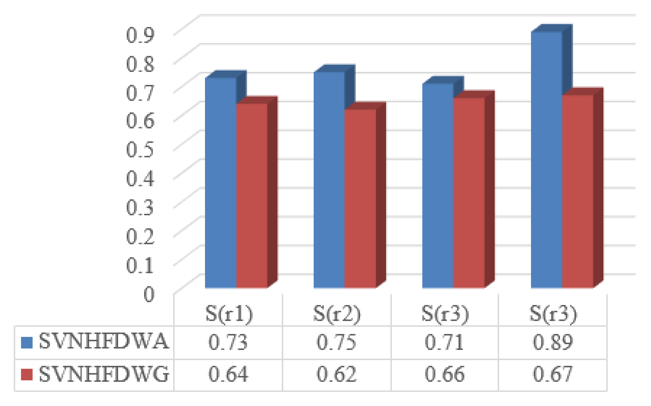
Rank the alternatives according to score function,
x 4 x 2 x 1 x 3
Step 5. 
Ranking of alternatives shows that x 4 is the best alternative among four alternatives.
If we solve the problem of making decisions based on numerous attributes by employing the SVNHFDWG operator, the process of creating decisions may be outlined in the following way:
Step 2. 
Compute the collective SVNHFN x i ( i = 1 , 2 , 3 , 4 ) for the alternatives A i γ ( i = 1 , 2 , 3 , 4 ) by utilizing the SVNHFDWG operator:
x i = SVNHFDWG ( x i 1 , x i 2 , , x i m ) = j = 1 m x i j w j = ϕ i 1 P i 1 , ϕ i 2 P i 2 , , ϕ i m P i m , φ i 1 I i 1 , φ i 2 I i 2 , , φ i m I i m , ψ i 1 N i 1 , ψ i 2 N i 2 , , ψ i m N i m
1 1 1 + j = 1 m w j 1 ϕ i j ϕ i j λ 1 / λ , 1 1 + j = 1 m w j φ i j 1 φ i j λ 1 / λ , 1 1 + j = 1 m w j ψ i j 1 ψ i j λ 1 / λ
x 1 = { 0.662 , 0.694 , 0.667 , 0.700 , 0.726 , 0.733 , 0.782 , 0.795 } , { 0.344 , 0.366 , 0.369 , 0.387 } , { 0.397 , 0.405 , 0.458 , 0.473 } x 2 = { 0.507 , 0.530 , 0.537 , 0.589 , 0.635 , 0.651 } , { 0.221 , 0.282 , 0.358 , 0.271 , 0.315 , 0.377 } , { 0.404 , 0.410 } x 3 = { 0.715 , 0.756 } , { 0.383 } , { 0.351 , 0.355 , 0.382 , 0.378 , 0.382 , 0.404 } x 4 = { 0.856 , 0.915 } , { 0.301 , 0.317 , 0.385 , 0.394 , 0.317 , 0.394 , 0.332 , 0.402 , 0.341 , 0.354 , 0.408 , 0.415 } , { 0.511 }
Step 3. 
Calculate the score function of x i ( i = 1 , 2 , 3 , 4 ) by using Equation (1); then, we obtain
S ( x 1 ) = 0.64
S ( x 2 ) = 0.62
S ( x 3 ) = 0.66
S ( x 4 ) = 0.67
Step 4. 
The score function provides real numbers to the alternatives, and these alternatives gained the ranking as follows. The score function assigns real numbers to every alternative, and the order in which these alternatives are arranged follow a usual order from higher values to lower values as follows:
x 4 x 3 x 1 x 2
Step 5. 
The ranking of alternatives clearly describes that x 4 is the top alternative among four alternatives.

5.2. Comparative Analysis

The symmetry of top alternative can be seen by using Algorithm 1 for SVNHFWA, SVNHFWG, SVNHFDWA and SVNHFDWG operators. On the other hand, the order in which the options are ranked is not entirely consistent. This demonstrates that the ranking of alternatives is determined to seek the top alternative and positions of remaining alternatives. The comparative analysis of this ranking of alternatives is expressed in Table 9.
Algorithm 1: Algorithm for SVNHF information using Dombi aggregation operators
Consider a set of alternatives A γ = { A 1 γ A 2 γ , , A n γ } and a set of criterion C = { C 1 , C 2 , , C m } . The decision maker D gives his/her own decision matrix D = ( x i j ) n × m in the form of SVNHFNs, x i j is given for alternatives A i γ A γ with respect to criterion C j C .
Step 1. Consider a decision matrix D = ( x i j ) n × m in the form of SVNHFNs.
Step 2. Compute the collective SVNHFN x i ( i = 1 , 2 , , n ) for the alternatives A i γ ( i = 1 , 2 , , n ) by utilizing the SVNHFDWA operator:
x i = SVNHFDWA ( x i 1 , x i 2 , , x i m ) = j = 1 m ( w j x i j ) = ϕ i 1 P i 1 , ϕ i 2 P i 2 , , ϕ i m P i m , φ i 1 I i 1 , φ i 2 I i 2 , , φ i m I i m , ψ i 1 N i 1 , ψ i 2 N i 2 , , ψ i m N i m
1 1 1 + j = 1 m w j ϕ i j 1 ϕ i j λ 1 / λ , 1 1 + j = 1 m w j 1 φ i j φ i j λ 1 / λ , 1 1 + j = 1 m w j 1 ψ i j ψ i j λ 1 / λ
or by utilizing the SVNHFDWG operator:
x i = SVNHFDWG ( x i 1 , x i 2 , , x i m ) = j = 1 m x i j w j = ϕ i 1 P i 1 , ϕ i 2 P i 2 , , ϕ i m P i m , φ i 1 I i 1 , φ i 2 I i 2 , , φ i m I i m , ψ i 1 N i 1 , ψ i 2 N i 2 , , ψ i m N i m
1 1 1 + j = 1 m w j 1 ϕ i j ϕ i j λ 1 / λ , 1 1 + j = 1 m w j φ i j 1 φ i j λ 1 / λ , 1 1 + j = 1 m w j ψ i j 1 ψ i j λ 1 / λ
Step 3. Compute the score function of the collective SVNHFNs x i ( i = 1 , 2 , , n ) by utilizing Equation (1).
Step 4. Using a score function, rank the alternatives.
Step 5. Choose the top alternative.
The comparison bar chart of ranking with SVNHFWA and SVNHFWG is shown in Figure 2.

6. Conclusions

SVNHFS is a robust fusion of an SVNS and HFS created for scenarios where each object has some possible values determined by truth-MD, indeterminacy, and falsity-MD. In this article, we propose an SVNHFDWA operator, SVNHFDWG operator, SVNHFDOWA operator, SVNHFDOWG operator, SVNHFDHA operator and SVNHFDHG operator. In addition, we proposed two innovative MADM techniques based on the SVNHFDWA and SVNHFDWG operators. The benefits of these methods are outlined in more detail below.
  • First, the SVNHFDWA and SVNHFDWG operators have significant properties such as idempotency, commutativity as well as boundedness and monotonity.
  • Second, the SVNHFDWA and SVNHFDWG operators can be converted to the previous AOs for SVNHFSs, which identify the versatility of proposed AOs.
  • Third, when compared to other existing approaches for MADM problems in an SVNHF environment, the results achieved by the SVNHFDWA and SVNHFDWG operators are reliable and accurate, which demonstrates their applicability in practical settings.
  • The techniques that are proposed for MADM in this paper are able to further acknowledge more association between attributes and alternatives, which demonstrates that they have a greater accuracy and a larger reference value than the techniques that are currently in use and that are unable to take into account the inter-relationships of attributes in practical applications. This means that the techniques that are proposed for MADM in this paper can further recognize more association between attributes.
  • A practical application of the proposed aggregation operators is also presented to examine symmetrical analysis in the selection of a feasible mobile robot (mobile charger) for vehicles.
  • It would be interesting to use the proposed AOs in future studies to deal with personalized individual semantics-based consistency control consensus problems in IDSS, consensus reaching with non-cooperative behavior management decision-making problems, and two-sided matching decision making with multi-granular and incomplete criteria weight information. In the context of this discussion on the constraints imposed by proposed AOs, there is no interaction between the degrees of membership, abstention, and non-membership. New hybrid structure of interactive and prioritized AOs may be seen being put into place on this side of the planned AOs.

Author Contributions

S.B., M.R.H. and M.R. worked on the methodology, conceptualization, and writing the original draft. M.R. and D.P. worked on software, validation, and investigation. F.S. and D.S. were responsible for the the project administration, supervision, and formal analysis. All authors have read and agreed to the published version of the manuscript.

Funding

This research received no external funding.

Institutional Review Board Statement

Not applicable.

Informed Consent Statement

Not applicable.

Data Availability Statement

Not applicable.

Conflicts of Interest

The authors declare no conflict of interest.

References

  1. Zadeh, L.A. Fuzzy sets. Inform. Control 1965, 8, 338–356. [Google Scholar] [CrossRef] [Green Version]
  2. Atanassov, K.T. Intuitionistic fuzzy sets. Fuzzy Set Syst. 1986, 20, 87–96. [Google Scholar] [CrossRef]
  3. Xu, Z. Intuitionistic fuzzy aggregation operators. IEEE Trans. Fuzzy Syst. 2007, 15, 1179–1187. [Google Scholar]
  4. Atanassov, K.; Gargov, G. Interval-valued intuitionistic fuzzy sets. Fuzzy Sets Syst. 1989, 31, 343–349. [Google Scholar] [CrossRef]
  5. Smarandache, F. A Unifying Field in Logics. Neutrosophy: Neutrosophic Probability, Set and Logic; American Research Press: Rehoboth, DE, USA, 1999. [Google Scholar]
  6. Wang, H.; Smarandache, F.; Zhang, Y.; Sunderraman, R. Single-Valued Neutrosophic Sets; Technical Sciences and Applied Mathematics; Infinite Study: Hurstville, Australia, 2012. [Google Scholar]
  7. Wang, H.; Smarandache, F.; Zhang, Y.Q.; Sunderraman, R. Interval Neutrosophic Sets and Logic: Theory and Applications in Computing; Hexis: Phoenix, AZ, USA, 2005; Volume 7. [Google Scholar]
  8. Torra, V.; Narukawa, Y. On hesitant fuzzy sets and decision. In Proceedings of the IEEE International Conference on Fuzzy Systems, Tianjin, China, 14–16 August 2009; pp. 1378–1382. [Google Scholar]
  9. Torra, V. Hesitant fuzzy sets. Int. J. Intell. Syst. 2010, 25, 529–539. [Google Scholar] [CrossRef]
  10. Ye, J. Multiple attribute decision making method under a single-valued neutrosophic hesitant fuzzy environment. J. Intell. Syst. 2015, 24, 23–36. [Google Scholar] [CrossRef]
  11. Liu, C.F.; Luo, Y.S. New aggregation operators of single-valued neutrosophic hesitant fuzzy set and their application in multi-attribute decision making. Pattern Anal. Appl. 2019, 22, 417–427. [Google Scholar] [CrossRef]
  12. Dombi, J. A general class of fuzzy operators, the demorgan class of fuzzy operators and fuzziness measures induced by fuzzy operators. Fuzzy Sets Syst. 1982, 8, 149–163. [Google Scholar] [CrossRef]
  13. Seikh, M.R.; Mandal, U. Intuitionistic fuzzy Dombi aggregation operators and their application to multiple attribute decision-making. Granul. Comput. 2021, 6, 473–488. [Google Scholar] [CrossRef]
  14. Liu, P.D.; Liu, J.L.; Chen, S.M. Some intuitionistic fuzzy Dombi Bonferroni mean operators and their application to multi-attribute group decision making. J. Oper. Res. Soc. 2017, 69, 1–26. [Google Scholar] [CrossRef]
  15. Wang, W.; Liu, X. Intuitionistic Fuzzy Information Aggregation Using Einstein Operations. IEEE Trans. Fuzzy Syst. 2012, 20, 923–938. [Google Scholar] [CrossRef]
  16. Yua, X.; Xu, Z. Prioritized intuitionistic fuzzy aggregation operators. Inf. Fusion 2013, 14, 108–116. [Google Scholar] [CrossRef]
  17. Alkenani, A.; Anjum, R.; Islam, S. Intuitionistic Fuzzy Prioritized Aggregation Operators Based on Priority Degrees with Application to Multicriteria Decision-Making. J. Funct. Spaces 2022, 2022, 4751835. [Google Scholar]
  18. Tan, C.; Chen, X. Intuitionistic fuzzy Choquet integral operator for multi-criteria decision making. Expert Syst. Appl. 2010, 37, 149–157. [Google Scholar] [CrossRef]
  19. Xu, Z. Approaches to multiple attribute group decision making based on intuitionistic fuzzy power aggregation operators. Knowl.-Based Syst. 2011, 24, 749–760. [Google Scholar] [CrossRef]
  20. Yang, W.; Chen, Z. The quasi-arithmetic intuitionistic fuzzy OWA operators. Knowl.-Based Syst. 2012, 27, 219–233. [Google Scholar] [CrossRef]
  21. Wu, L.; Wei, G.; Wu, J.; Wei, C. Some Interval-Valued Intuitionistic Fuzzy Dombi Heronian Mean Operators and their Application for Evaluating the Ecological Value of Forest Ecological Tourism Demonstration Areas. Int. J. Environ. Res. Public Health 2020, 17, 829. [Google Scholar] [CrossRef] [Green Version]
  22. Wu, L.; Wei, G.; Gao, H.; Wei, Y. Some Interval-Valued Intuitionistic Fuzzy Dombi Hamy Mean Operators and Their Application for Evaluating the Elderly Tourism Service Quality in Tourism Destination. Mathematics 2018, 6, 294. [Google Scholar] [CrossRef] [Green Version]
  23. Wang, Q.; Sun, H. Interval-Valued Intuitionistic Fuzzy Einstein Geometric Choquet Integral Operator and Its Application to Multiattribute Group Decision-Making. Math. Probl. Eng. 2018, 2018, 9364987. [Google Scholar] [CrossRef]
  24. Wang, W.; Liu, X. Interval-valued intuitionistic fuzzy hybrid weighted averaging operator based on Einstein operation and its application to decision making. J. Intell. Fuzzy Syst. 2013, 25, 279–290. [Google Scholar] [CrossRef]
  25. Liu, P. Some Hamacher Aggregation operators based on the interval-valued intuitionistic fuzzy numbers and their application to group decision making. IEEE Trans. Fuzzy Syst. 2013, 22, 83–97. [Google Scholar] [CrossRef]
  26. Akram, M.; Dudek, W.A.; Dar, J.M. Pythagorean Dombi fuzzy aggregation operators with application in multi criteria decision-making. Int. J. Intell. Syst. 2019, 34, 3000–3019. [Google Scholar] [CrossRef]
  27. Jana, C.; Senapati, T.; Pal, M. Pythagorean fuzzy Dombi aggregation operators and its applications in multiple attribute decision-making. Int. J. Intell. Syst. 2019, 34, 1–21. [Google Scholar] [CrossRef]
  28. Rahman, K.; Abdullah, S.; Ali, A.; Amin, F. Pythagorean Fuzzy Einstein Hybrid Averaging Aggregation Operator and its Application to Multiple-Attribute Group Decision Making. J. Intell. Syst. 2018, 40, 180–187. [Google Scholar] [CrossRef]
  29. Khan, M.S.A.; Abdullah, S.; Ali, A.; Amin, F. Pythagorean fuzzy prioritized aggregation operators and their application to multi-attribute group decision making. Granul. Comput. 2019, 4, 249–263. [Google Scholar] [CrossRef]
  30. Farid, H.M.A.; Riaz, M. Pythagorean fuzzy prioritized aggregation operators with priority degrees for multi-criteria decision-making. Int. J. Intell. Comput. Cybern. 2022, 15, 510–539. [Google Scholar] [CrossRef]
  31. Wang, L.; Li, N. Pythagorean fuzzy interaction power Bonferroni mean aggregation operators in multiple attribute decision making. Int. J. Intell. Syst. 2020, 35, 150–183. [Google Scholar] [CrossRef]
  32. Liang, D.; Zhang, Y.; Xu, Z.; Darko, A.P. Pythagorean fuzzy Bonferroni mean aggregation operator and its accelerative calculating algorithm with the multithreading. Int. J. Intell. Syst. 2018, 33, 615–633. [Google Scholar] [CrossRef]
  33. Chen, J.; Ye, J. Some Single-Valued Neutrosophic Dombi Weighted Aggregation Operators for Multiple Attribute Decision-Making. Symmetry 2017, 9, 82. [Google Scholar] [CrossRef]
  34. Jana, C.; Pal, M. Multi-criteria decision making process based on some single-valued neutrosophic Dombi power aggregation operators. Soft Comput. 2021, 25, 5055–5072. [Google Scholar] [CrossRef]
  35. Wei, G.; Wei, Y. Some single-valued neutrosophic dombi prioritized weighted aggregation operators in multiple attribute decision making. J. Intell. Fuzzy 2018, 35, 2001–2013. [Google Scholar] [CrossRef]
  36. Liu, P.; Khan, Q.; Mahmood, T. Multiple-attribute decision making based on single-valued neutrosophic Schweizer-Sklar prioritized aggregation operator. Cogn. Syst. Res. 2019, 57, 175–196. [Google Scholar] [CrossRef]
  37. Farid, H.M.A.; Garg, H.; Riaz, M.; Garcia, G.S. Multi-criteria group decision-making algorithm based on single-valued neutrosophic Einstein prioritized aggregation operators and its applications. Manag. Decis. 2022. [Google Scholar] [CrossRef]
  38. He, X. Typhoon disaster assessment based on Dombi hesitant fuzzy information aggregation operators. Nat. Hazards J. Int. Soc. Prev. Mitig. Nat. Hazards 2018, 90, 1153–1175. [Google Scholar] [CrossRef]
  39. Liu, P.; Saha, A.; Dutta, D.; Kar, S. Multi-Attribute Decision-Making Using Hesitant Fuzzy Dombi–Archimedean Weighted Aggregation Operators. Int. J. Comput. Intell. Syst. 2021, 14, 386–411. [Google Scholar] [CrossRef]
  40. Saha, A.; Dutta, D.; Kar, S. Some new hybrid hesitant fuzzy weighted aggregation operators based on Archimedean and Dombi operations for multi-attribute decision making. Neural Comput. Appl. 2021, 33, 8753–8776. [Google Scholar] [CrossRef]
  41. Yu, Q.; Hou, F.; Zhai, Y.; Du, Y. Some Hesitant Fuzzy Einstein Aggregation Operators and Their Application to Multiple Attribute Group Decision Making. Int. J. Intell. Syst. 2015, 31, 722–746. [Google Scholar] [CrossRef]
  42. Zhou, L.; Zhao, X.; Wei, G. Hesitant fuzzy Hamacher Aggregation operators and their application to multiple attribute decision making. J. Intell. Fuzzy Syst. 2014, 26, 2689–2699. [Google Scholar] [CrossRef]
  43. Li, X.; Zhang, X. Single-Valued Neutrosophic Hesitant Fuzzy Choquet Aggregation Operators for Multi-Attribute Decision Making. Symmetry 2018, 10, 50. [Google Scholar] [CrossRef] [Green Version]
  44. Wang, R.; Li, Y. Generalized Single-Valued Neutrosophic Hesitant Fuzzy Prioritized Aggregation Operators and Their Applications to Multiple Criteria Decision-Making. Information 2018, 9, 10. [Google Scholar] [CrossRef] [Green Version]
  45. Wang, L.; Bao, Y.L. Multiple-Attribute Decision-Making Method Based on Normalized Geometric Aggregation Operators of Single-Valued Neutrosophic Hesitant Fuzzy Information. Complexity 2021, 2021, 5580761. [Google Scholar] [CrossRef]
  46. Hanif, M.Z.; Yaqoob, N.; Riaz, M.; Aslam, M. Linear Diophantine fuzzy graphs with new decision-making approach. AIMS Math. 2022, 7, 14532–14556. [Google Scholar] [CrossRef]
  47. Prakash, K.; Parimala, M.; Garg, H.; Riaz, M. Lifetime prolongation of a wireless charging sensor network using a mobile robot via linear Diophantine fuzzy graph environment. Complex Intell. Syst. 2022, 8, 2419–2434. [Google Scholar] [CrossRef]
  48. Mohamed, N.; Aymen, F.; Mouna, B.H.; Alassaad, S. Review on autonomous charger for EV and HEV. In Proceedings of the 2017 IEEE International Conference on Green Energy Conversion Systems (GECS), Hammamet, Tunisia, 23–25 March 2017; pp. 1–6. [Google Scholar]
  49. Tang, Y.M.; Zhang, L.; Bao, G.Q.; Ren, F.J.; Pedrycz, W. Symmetric implicational algorithm derived from intuitionistic fuzzy entropy. Iran. J. Fuzzy Syst. 2022, 19, 27–44. [Google Scholar]
  50. Wang, Z.J. A Representable Uninorm-Based Intuitionistic Fuzzy Analytic Hierarchy Process. IEEE Trans. Fuzzy Syst. 2020, 28, 2555–2569. [Google Scholar] [CrossRef]
  51. Lodwick, W.A.; Kacprzyk, J. (Eds.) Fuzzy Optimization: Recent Advances and Applications; Springer: Berlin/Heidelberg, Germany, 2010; Volume 254. [Google Scholar]
  52. Riaz, M.; Farid, H.M.A. Picture fuzzy aggregation approach with application to third-party logistic provider selection process. Rep. Mech. Eng. 2022, 3, 318–327. [Google Scholar] [CrossRef]
  53. Karaaslan, F.; Çağman, N. Parameter trees based on soft set theory and their similarity measures. Soft Comput. 2022, 26, 4629–4639. [Google Scholar] [CrossRef]
  54. Karamasa, Ç.; Karabasevic, D.; Stanujkic, D.; Kookhdan, A.; Mishra, A.; Ertürk, M. An extended single-valued neutrosophic AHP and MULTIMOORA method to evaluate the optimal training aircraft for flight training organizations. Facta Univ. Ser. Mech. Eng. 2021, 19, 555–578. [Google Scholar] [CrossRef]
  55. Ali, Z.; Mahmood, T.; Ullah, K.; Khan, Q. Einstein Geometric Aggregation Operators using a Novel Complex Interval-valued Pythagorean Fuzzy Setting with Application in Green Supplier Chain Management. Rep. Mech. Eng. 2021, 2, 105–134. [Google Scholar] [CrossRef]
  56. Bozanic, D.; Milic, A.; Tešic, D.; Salabun, W.; Pamucar, D. D numbers—FUCOM—Fuzzy RAFSI model for selecting the group of construction machines for enabling mobility. Facta Univ. Ser. Mech. Eng. 2021, 19, 447–471. [Google Scholar]
  57. Ashraf, A.; Ullah, K.; Hussain, A.; Bari, M. Interval-Valued Picture Fuzzy Maclaurin Symmetric Mean Operator with application in Multiple Attribute Decision-Making. Rep. Mech. Eng. 2022, 3, 301–317. [Google Scholar] [CrossRef]
  58. Sahu, R.; Dash, S.R.; Das, S. Career selection of students using hybridized distance measure based on picture fuzzy set and rough set theory. Decis. Mak. Appl. Manag. Eng. 2021, 4, 104–126. [Google Scholar] [CrossRef]
  59. Shi, L.; Ye, J. Dombi aggregation operators of neutrosophic cubic sets for multiple attribute decision-making. Algorithms 2018, 11, 29. [Google Scholar] [CrossRef]
  60. Biswas, P.; Pramanik, S.; Giri, B.C. GRA Method of Multiple Attribute Decision Making with Single Valued Neutrosophic Hesitant Fuzzy Set Information. New Trends Neutrosophic Theory Appl. 2016, 55–63. [Google Scholar]
Figure 1. Sensor network for mobile robot charger.
Symmetry 14 02271 g001
Figure 2. Comparison bar chart of ranking with SVNHFWA and SVNHFWG.
Symmetry 14 02271 g002
Table 1. Operators for fuzzy sets.
Fuzzy SetOperatorReference
IFSDombi aggregation operator[13]
Dombi Bonferroni mean operators[14]
Einstein aggregation operators[15]
Prioritized aggregation operators[16]
Prioritized AO with priority degrees[17]
Choquet integral operator[18]
Power AAO and GAO[19]
Quasi AO[20]
IVIFSDombi Heronian mean AO[21]
Dombi Hamy mean operators[22]
Einstein Geometric Choquet Integral operator[23]
Hybrid WAO based on Einstein operation[24]
Hamacher AO[25]
PFSDombi aggregation AO[26,27]
Einstein hybrid averaging aggregation operator[28]
Prioritized aggregation operators[29]
Prioritized aggregation operators based on priority degrees[30]
Interaction power Bonferroni mean AO[31]
Bonferroni mean AO[32]
SVNSDombi weighted aggregation operators[33]
Dombi power aggregation operators[34]
Dombi prioritized weighted aggregation operators[35]
Schweizer–Sklar prioritized aggregation operator[36]
Einstein prioritized aggregation operators[37]
HFSDombi aggregation operators[38]
Dombi–Archimedean weighted aggregation operators[39,40]
Einstein aggregation operators[41]
Hamacher Aggregation operators[42]
SVNHFSChoquet aggregation operators[43]
Prioritized aggregation operators[44]
Normalized geometric aggregation operators[45]
Table 2. SVNHFNs.
Table 2. SVNHFNs.
x 1 { 0.432 , 0.567 } , { 0.111 } , { 0.334 }
x 2 { 0.519 , 0.678 , 0.800 } , { 0.200 , 0.350 } , { 0.156 , 0.259 }
x 3 { 0.750 } , { 0.290 , 0.381 , 0.476 } , { 0.500 }
Table 3. Aggregated SVNHFNs based on SVNHFDWA operator.
ParameterAggregated SVNHFNs
λ = 1 { 0.639 , 0.680 , 0.736 , 0.656 , 0.694 , 0.745 } , { 0.186 , 0.198 , 0.207 , 0.216 , 0.232 , 0.244 } , { 0.264 , 0.345 }
λ = 2 { 0.671 , 0.678 , 0.697 , 0.703 , 0.754 , 0.756 } , { 0.169 , 0.174 , 0.175 , 0.184 , 0.189 , 0.192 } , { 0.227 , 0.326 }
λ = 4 { 0.706 , 0.715 , 0.769 , 0.707 , 0.716 , 0.769 } , { 0.147 , 0.147 , 0.147 , 0.150 , 0.150 , 0.150 } , { 0.193 , 0.303 }
λ = 5 { 0.714 , 0.720 , 0.773 , 0.715 , 0.720 , 0.773 } , { 0.140 , 0.140 , 0.140 , 0.141 , 0.141 , 0.141 } , { 0.186 , 0.296 }
λ = 10 { 0.732 , 0.733 , 0.784 , 0.732 , 0.733 , 0.784 } , { 0.125 , 0.125 , 0.125 , 0.125 , 0.125 , 0.125 } , { 0.170 , 0.279 }
λ = 20 { 0.741 , 0.741 , 0.791 , 0.741 , 0.741 , 0.791 } , { 0.118 , 0.118 , 0.118 , 0.118 , 0.118 , 0.118 } , { 0.163 , 0.269 }
λ = 50 { 0.747 , 0.747 , 0.797 , 0.747 , 0.747 , 0.797 } , { 0.114 , 0.114 , 0.114 , 0.114 , 0.114 , 0.114 } , { 0.158 , 0.263 }
λ = 100 { 0.748 , 0.748 , 0.798 , 0.748 , 0.748 , 0.798 } , { 0.112 , 0.112 , 0.112 , 0.112 , 0.112 , 0.112 } , { 0.158 , 0.261 }
Table 4. Aggregated SVNHFNs based on SVNHFDWG operator.
ParameterAggregated SVNHFNs
λ = 1 { 0.560 , 0.607 , 0.614 , 0.671 , 0.645 , 0.708 } , { 0.220 , 0.267 , 0.325 , 0.277 , 0.318 , 0.368 } , { 0.371 , 0.393 }
λ = 2 { 0.531 , 0.588 , 0.573 , 0.658 , 0.586 , 0.684 } , { 0.233 , 0.296 , 0.374 , 0.293 , 0.336 , 0.398 } , { 0.408 , 0.416 }
λ = 4 { 0.499 , 0.566 , 0.516 , 0.636 , 0.518 , 0.645 } , { 0.251 , 0.330 , 0.420 , 0.310 , 0.352 , 0.426 } , { 0.445 , 0.446 }
λ = 5 { 0.490 , 0.559 , 0.500 , 0.627 , 0.501 , 0.632 } , { 0.257 , 0.339 , 0.431 , 0.315 , 0.356 , 0.434 } , { 0.455 , 0.456 }
λ = 10 { 0.465 , 0.543 , 0.466 , 0.600 , 0.466 , 0.601 } , { 0.272 , 0.360 , 0.453 , 0.328 , 0.364 , 0.453 } , { 0.477 , 0.477 }
λ = 20 { 0.449 , 0.532 , 0.449 , 0.584 , 0.449 , 0.584 } , { 0.281 , 0.370 , 0.465 , 0.338 , 0.371 , 0.465 } , { 0.489 , 0.489 }
λ = 50 { 0.439 , 0.524 , 0.439 , 0.574 , 0.439 , 0.574 } , { 0.286 , 0.377 , 0.471 , 0.345 , 0.377 , 0.471 } , { 0.495 , 0.495 }
λ = 100 { 0.435 , 0.522 , 0.435 , 0.570 , 0.435 , 0.570 } , { 0.288 , 0.379 , 0.474 , 0.348 , 0.379 , 0.474 } , { 0.498 , 0.498 }
Table 5. Aggregated SVNHFNs based on SVNHFDOWA operator.
ParameterAggregated SVNHFNs
λ = 1 { 0.634 , 0.666 , 0.711 , 0.658 , 0.686 , 0.727 } , { 0.173 , 0.191 , 0.183 , 0.203 , 0.191 , 0.212 } , { 0.290 , 0.355 }
λ = 2 { 0.669 , 0.689 , 0.736 , 0.679 , 0.697 , 0.741 } , { 0.157 , 0.165 , 0.160 , 0.168 , 0.162 , 0.170 } , { 0.249 , 0.338 }
λ = 4 { 0.705 , 0.7120 . 758 , 0.707 , 0.713 , 0.759 } , { 0.138 , 0.139 , 0.138 , 0.140 , 0.138 , 0.140 } , { 0.206 , 0.314 }
λ = 5 { 0.714 , 0.718 , 0.764 , 0.715 , 0.719 , 0.764 } , { 0.133 , 0.133 , 0.133 , 0.133 , 0.133 , 0.133 } , { 0.196 , 0.306 }
λ = 10 { 0.732 , 0.733 , 0.778 , 0.732 , 0.733 , 0.778 } , { 0.122 , 0.122 , 0.122 , 0.122 , 0.122 , 0.122 } , { 0.175 , 0.286 }
λ = 20 { 0.741 , 0.741 , 0.789 , 0.741 , 0.741 , 0.789 } , { 0.116 , 0.116 , 0.116 , 0.116 , 0.116 , 0.116 } , { 0.165 , 0.273 }
λ = 50 { 0.747 , 0.747 , 0.796 , 0.747 , 0.747 , 0.796 } , { 0.113 , 0.113 , 0.113 , 0.113 , 0.113 , 0.113 } , { 0.160 , 0.264 }
λ = 100 { 0.748 , 0.748 , 0.798 , 0.748 , 0.748 , 0.798 } , { 0.112 , 0.112 , 0.112 , 0.112 , 0.112 , 0.112 } , { 0.158 , 0.262 }
Table 6. Aggregated SVNHFNs based on SVNHFDOWG operator.
ParameterAggregated SVNHFNs
λ = 1 { 0.548 , 0.584 , 0.604 , 0.613 , 0.658 , 0.683 } , { 0.212 , 0.298 , 0.320 , 0.255 , 0.261 , 0.351 } , { 0.383 , 0.399 }
λ = 2 { 0.518 , 0.543 , 0.551 , 0.595 , 0.644 , 0.661 } , { 0.229 , 0.324 , 0.372 , 0.276 , 0.294 , 0.390 } , { 0.413 , 0.419 }
λ = 4 { 0.487 , 0.4960 . 497 , 0.573 , 0.622 , 0.627 } , { 0.249 , 0.346 , 0.420 , 0.298 , 0.330 , 0.424 } , { 0.446 , 0.447 }
λ = 5 { 0.478 , 0.484 , 0.484 , 0.566 , 0.614 , 0.617 } , { 0.256 , 0.351 , 0.431 , 0.304 , 0.339 , 0.433 } , { 0.456 , 0.456 }
λ = 10 { 0.457 , 0.458 , 0.458 , 0.549 , 0.592 , 0.593 } , { 0.272 , 0.363 , 0.453 , 0.321 , 0.360 , 0.453 } , { 0.477 , 0.477 }
λ = 20 { 0.445 , 0.445 , 0.445 , 0.536 , 0.580 , 0.580 } , { 0.281 , 0.371 , 0.465 , 0.334 , 0.370 , 0.465 } , { 0.486 , 0.486 }
λ = 50 { 0.437 , 0.437 , 0.437 , 0.526 , 0.572 , 0.572 } , { 0.286 , 0.377 , 0.471 , 0.344 , 0.377 , 0.471 } , { 0.495 , 0.495 }
λ = 100 { 0.435 , 0.435 , 0.435 , 0.522 , 0.570 , 0.570 } , { 0.288 , 0.379 , 0.474 , 0.347 , 0.379 , 0.474 } , { 0.498 , 0.498 }
Table 7. Criterion for mobile robot charger.
CriterionSignificance of Criterion
C 1 
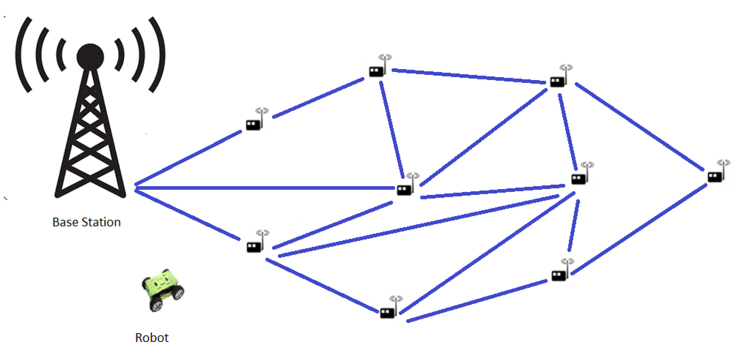
Type of mobile charger (MC).
C 2 Each individual node that makes up a wireless sensor system is provided with its
own wireless power receiver.
C 3 The energy generation station is located in the base station. It is in charge of determining
the amount of energy that is required for each node and supplying that information to the
robot along with the nodes’ respective positions.
Table 8. Tabular representation of SVNHFNs.
Alternatives C 1
A 1 γ { 0.678 , 0.801 } , { 0.222 , 0.333 } , { 0.444 , 0.550 }
A 2 γ { 0.432 , 0.567 } , { 0.111 } , { 0.334 }
A 3 γ { 0.676 , 0.768 } , { 0.382 } , { 0.449 }
A 4 γ { 0.980 } , { 0.100 , 0.230 , 0.320 } , { 0.200 }
Alternatives C 2
A 1 γ { 0.810 , 0.900 } , { 0.215 , 0.356 } , { 0.400 }
A 2 γ { 0.519 , 0.678 , 0.800 } , { 0.200 , 0.350 } , { 0.156 , 0.259 }
A 3 γ { 0.856 } , { 0.358 } , { 0.200 , 0.380 }
A 4 γ { 0.900 } , { 0.450 , 0.550 } , { 0.660 }
Alternatives C 3
A 1 γ { 0.600 , 0.750 } , { 0.444 } , { 0.121 , 0.344 }
A 2 γ { 0.750 } , { 0.290 , 0.381 , 0.476 } , { 0.500 }
A 3 γ { 0.706 } , { 0.400 } , { 0.150 , 0.200 , 0.350 }
A 4 γ { 0.789 , 0.890 } , { 0.159 , 0.260 } , { 0.370 }
Table 9. Comparison table.
OperatorRankingOptimal Alternative
SVNHFWA x 4 x 2 x 1 x 3 x 4
SVNHFWG x 4 x 3 x 1 x 2 x 4
SVNHFDWA x 4 x 2 x 1 x 3 x 4
SVNHFDWG x 4 x 3 x 1 x 2 x 4
SVNHFCOA [43] x 4 x 3 x 2 x 1 x 4
GSVNHFPWA [44] x 4 x 3 x 1 x 2 x 4
Publisher’s Note: MDPI stays neutral with regard to jurisdictional claims in published maps and institutional affiliations.

