Article

Perturbed Newton Methods for Solving Nonlinear Equations with Applications

1
Department of Computing and Mathematical Sciences, Cameron University, Lawton, OK 73505, USA
2
Department of Mathematics, University of Houston, Houston, TX 77204, USA
3
Department of Theory of Optimal Processes, Ivan Franko National University of Lviv, Universytetska Str. 1, 79000 Lviv, Ukraine
*
Author to whom correspondence should be addressed.
Symmetry 2022, 14(10), 2206; https://doi.org/10.3390/sym14102206
Submission received: 9 September 2022 / Revised: 15 October 2022 / Accepted: 17 October 2022 / Published: 20 October 2022

Abstract

:
Symmetries play an important role in the study of a plethora of physical phenomena, including the study of microworlds. These phenomena reduce to solving nonlinear equations in abstract spaces. Therefore, it is important to design iterative methods for approximating the solutions, since closed forms of them can be found only in special cases. Several iterative methods were developed whose convergence was established under very general conditions. Numerous applications are also provided to solve systems of nonlinear equations and differential equations appearing in the aforementioned areas. The ball convergence analysis was developed for the King-like and Jarratt-like families of methods to solve equations under the same set of conditions. Earlier studies have used conditions up to the fifth derivative, but they failed to show the fourth convergence order. Moreover, no error distances or results on the uniqueness of the solution were given either. However, we provide such results involving the derivative only appearing on these methods. Hence, we have expanded the usage of these methods. In the case of the Jarratt-like family of methods, our results also hold for Banach space-valued equations. Moreover, we compare the convergence ball and the dynamical features both theoretically and in numerical experiments.
MSC:
37N30; 65H05; 65H10; 30C15

1. Introduction

Let M = R or C and T M be a non-empty, convex and open set. We denote by B ¯ ( q * , μ ) the closure of the open ball B ( q * , μ ) with radius μ > 0 and center q * M . Suppose the set { B L : M M linear and bounded operators} is denoted by L ( M , M ) . Consider the non-linear equation
F ( q ) = 0 ,
where F : T M M is differentiable. Nonlinear equations of the type (1) are often used in science and other practical domains to tackle a variety of very challenging problems from diverse disciplines. Notice that solving these equations is a difficult process; the answer has only been found analytically in a small number of situations. As a result, iterative procedures are often utilized to solve these equations. The job of developing a successful iterative approach for tackling Equation (1) is a great challenge. A traditional technique, Newton’s iterative technique, is the one that is most commonly used to solve this problem. More results on advanced forms, in terms of efficiency and convergence order, of popular methods such as Newton’s, Jarratt’s, King’s and Chebyshev’s methods, are presented in [1,2,3,4,5,6,7,8,9]. Chun [10] developed fourth-order classes of new modifications of King’s family of methods [11] for solving nonlinear equations. These methods involve two function evaluations and one of its first derivatives per iteration. Additionally, as a special variant of King’s method, the classical Traub–Ostrowski method was derived. Wang et al. [12] presented a sixth-order variant of Jarratt’s method, which requires the evaluation of the function at an additional point in the iteration procedure of Jarratt’s method [13]. A new family of fourth-order methods independent of the second derivative was introduced by Ghanbari in [14]. This family generates the King’s family and some other well-known methods as specific cases. Grau-Sánchez and Gutiérrez [15], by using Obreshkov-like techniques, described two families of zero-finding iterative approaches. An efficient family of nonlinear system solvers was suggested by Cordero et al. [16] using a reduced composition technique on Newton’s and Jarratt’s methods. Sharma et al. [17] composed two weighted-Newton steps to construct an efficient, fourth-order weighted-Newton method to solve nonlinear systems. Sharma and Arora [18] introduced iterative methods of fourth and sixth convergence order for solving nonlinear systems. Two bi-parametric fourth-order families of predictor-corrector iterative solvers are given in [19]. Solaiman et al. [20] proposed a modified class of fourth and eighth-convergence order iterative methods based on King’s method for nonlinear equations. In each iteration, three function evaluations are required for the fourth-order methods, and the eighth-order methods require four evaluations. Other results related to the convergence and dynamics of iterative formulas can be found in [3,21,22,23,24,25,26,27,28,29].
This paper deals with a comparison of the convergence balls and the complex dynamical features between the King-like and Jarratt-like families of methods. These methods are as follows:
King-like family of methods (KLFM):
y n = q n F ( q n ) 1 F ( q n ) q n + 1 = y n A n 1 B n F ( q n ) 1 F ( y n )
and
Jarratt-like family of methods (JLFM):
y n = q n α F ( q n ) 1 F ( q n ) q n + 1 = y n γ C n 1 H n ( y n q n ) ,
where α , β , γ , δ M ,
A n = F ( q n ) + ( δ 2 ) F ( y n ) , B n = F ( q n ) + δ F ( y n ) , C n = I + β H n
and
H n = H ( y n , q n ) = F ( q n ) 1 ( F ( y n ) F ( q n ) ) .
If α = 1 , β = 3 2 , γ = 3 4 and δ [ 0 , 2 ] , methods (2) and (3) reduce to the ones studied in [2,11,13], where it was shown they are of fourth-order using fifth derivative and Taylor expansions. As such results require derivatives of higher orders, these methods are very hard to execute, since their scope of application is small. Notice, however, those derivatives of orders higher than one do not appear in these methods. Hence, the earlier results limit the applicability of these methods to equations containing functions that are at least five times differentiable, although they may converge. Hence, their applicability is restricted. To support our argument, we consider the following motivational function
F ( q ) = q 3 ln ( q 2 ) + q 5 q 4 , if q 0 0 , if q = 0 ,
where M = R and F is defined on T = [ 1 2 , 3 2 ] . Then, it is extremely important to emphasize that F is unbounded. As a consequence, the previous convergence findings for KLFM and JKLM, which are based on F ( v ) , are invalid in this case. Additionally, these convergence results supply negligible information regarding the limits on error q n q * , the convergence domain and about the whereabouts of the solution q * . We need the ball analysis of iterative methods for determining the convergence radii, establishing error bounds and calculating the region in which q * is unique. The most significant benefit of the ball analysis is that it simplifies the very demanding task of selecting a starting point. Having this perspective, we are encouraged to analyze and compare the balls of convergence of KLFM and JKLM under the same set of assumptions based on just the first derivative of F, which only appears in these methods. In addition to providing the error estimates q n q * and convergence radii, the convergence theorems that we established also offer a correct location of the solution q * . Notice also that the local convergence results are important, since they demonstrate the degree of difficulty in choosing the initial points. The dynamic comparison between these methods is also presented.
It is worth noticing that methods (2)–(4) are explicit. We refer the reader to [30,31,32] for important implicit methods. This type of method is out of the scope of this paper. However, we plan to study such methods in our future research, since they provide better stability during data processing along the same lines.
Various portions of this paper may be described as follows: Section 2 discusses the key convergence theorems on the ball analysis of KLFM and JFLM. Comparison of attraction basins for these methods is the main content of Section 3. Section 4 is devoted to numerical applications of various kinds. Section 5 contains the final remarks of this research.

2. Ball Comparison

We first present the ball convergence analysis for KLMF. Let S = [ 0 , ) .
Suppose function(s):
(i)
ω 0 ( t ) 1
has a minimal zero ρ 0 S \ { 0 } for function ω 0 : S S that is non-decreasing and continuous. Set S 0 = [ 0 , ρ 0 ) .
(ii)
h 1 ( t ) 1
has a minimal zero d 1 S 0 \ { 0 } , where function ω : [ 0 , 2 ρ 0 ) S is non-decreasing and continuous and h 1 : S 0 S is defined by
h 1 ( t ) = 0 1 ω ( ( 1 θ ) t ) d θ 1 ω 0 ( t ) .
(iii)
ω 0 ( h 1 ( t ) ) 1 and p ( t ) 1
have minimal zeros ρ 1 and ρ p S 0 \ { 0 } , respectively, where ω 1 : S 0 S is non-decreasing and continuous, and p : S 0 S is defined by
p ( t ) = 0 1 ω 0 ( θ t ) d θ + | δ 2 | 0 1 ω 1 ( θ h 1 ( t ) t ) d θ h 1 ( t ) .
Set ρ = min { ρ 1 , ρ p } and S 1 = [ 0 , ρ ) .
(iv)
h 2 ( t ) 1
has a minimal zero d 2 S 1 \ { 0 } , where h 2 : S 1 S is defined by
h 2 ( t ) = [ 0 1 ω ( ( 1 θ ) h 1 ( t ) t ) d θ 1 ω 0 ( h 1 ( t ) t ) + ( ω 0 ( t ) + ω 0 ( h 1 ( t ) t ) ) 0 1 ω 1 ( θ h 1 ( t ) t ) d θ ( 1 ω 0 ( t ) ) ( 1 ω 0 ( h 1 ( t ) t ) ) + 2 0 1 ω 1 ( θ h 1 ( t ) t ) d θ ( 1 ω 0 ( t ) ) ( 1 p ( t ) ) ] h 1 ( t ) .
Then, parameter d is defined by
d = min { d m } , m = 1 , 2
which shall be shown to be a convergence radius for KLMF. Set S 2 = [ 0 , d ) .
Notice that it is implied by (5)
0 ω 0 ( t ) < 1 ,
0 ω 0 ( h 1 ( t ) t ) < 1 ,
0 p ( t ) < 1
and
0 h m ( t ) < 1 , m = 1 , 2 ,
are satisfied if t S 2 .
The developed conditions ( C ) play a role in the ball convergence analysis of KLFM if functions ω are as given previously, and q * is a simple zero of F.
Suppose:
( C 1 )
F ( q * ) 1 ( F ( v ) F ( q * ) ) ω 0 ( v q * )
for each v T . Set T 0 = T B ( q * , ρ 0 ) .
( C 2 )
F ( q * ) 1 ( F ( u ) F ( z ) ) ω ( u z )
and
F ( q * ) 1 F ( z ) ω 1 ( z q * )
for each u , z T 0 .
( C 3 )
B ¯ ( q * , d ˜ ) T for some d ˜ to be given the latter.
( C 4 )
There exists d * d ˜ satisfying
0 1 ω 0 ( θ d * ) d θ < 1 .
Set T 1 = T B ¯ ( q * , d * ) .
Next, the main ball convergence for KLFM is given utilizing conditions (C).
Theorem 1.
Under conditions (C) for d ˜ = d , choose starting point q 0 B ( q * , d ) \ { q * } . Then, we get lim n q n = q * , which is the only zero of F in the domain T 1 given in ( C 4 ) .
Proof. 
Mathematical induction on i shall establish items
y i q * h 1 ( q i q * ) q i q * q i q * < d
q i + 1 q * h 2 ( q i q * ) q i q * q i q * .
Let q B ( q * , d ) \ { q * } . Using (5), (6) and ( C 1 ) , we obtain
F ( q * ) 1 ( F ( q ) F ( q * ) ) ω 0 ( q q * ) ω 0 ( d ) < 1
implying with a lemma due to Banach on linear operations with inverses [3,33] that F ( q ) is invertible with
F ( q ) 1 F ( q * ) 1 1 ω 0 ( q q * ) .
Notice that we now have that y 0 is well defined by the first substep of KLFM if n = 0 , from which we can also write
y 0 q * = q 0 q * F ( q 0 ) 1 F ( q 0 ) = ( F ( q 0 ) 1 F ( q * ) ) 0 1 F ( q * ) 1 ( F ( q * + θ ( q 0 q * ) ) F ( q 0 ) ) d θ ( q 0 q * ) .
By (5), (9) (for m = 1 ), (13) (for q = q 0 ), ( C 2 ) , ( C 3 ) and (14), we have
y 0 q * 0 1 ω ( ( 1 θ ) q 0 q * ) d θ q 0 q * 1 ω 0 ( q 0 q * ) h 1 ( q 0 q * ) q 0 q * q 0 q * < d
showing (10) for i = 0 and y 0 B ( q * , d ) .
Next, we shall establish the invertibility of A 0 provided that q 0 q * (otherwise, the proof for items (10) and (11) is terminated). In view of (5), (8), ( C 2 ) and (15), we have
( F ( q * ) ( q 0 q * ) ) 1 ( F ( q 0 ) F ( q * ) F ( q * ) ( q 0 q * ) + ( δ 2 ) ( F ( y 0 ) F ( q * ) ) ) 1 q 0 q * 0 1 F ( q * ) 1 F ( q * + θ ( q 0 q * ) ) F ( q * ) ) d θ q 0 q * + | δ 2 | 0 1 F ( q * ) 1 F ( q * + θ ( y 0 q * ) ) d θ y 0 q * ] 0 1 ω 0 ( θ q 0 q * ) d θ + | δ 2 | 0 1 ω 1 ( θ h 1 ( q 0 q * ) q 0 q * d θ h 1 ( q 0 q * ) = p ( q 0 q * ) p ( d ) < 1 ,
so
A 0 1 F ( q * ) 1 1 p ( q 0 q * ) ,
and q 1 is well defined by the second substep of KLFM, from which we can also write
q 1 q * = y 0 q * F ( y 0 ) 1 F ( y 0 ) + F ( y 0 ) 1 F ( y 0 ) A 0 1 B 0 F ( q 0 ) 1 F ( y 0 ) + F ( q 0 ) 1 F ( y 0 ) F ( q 0 ) 1 F ( y 0 ) = y 0 q * F ( y 0 ) 1 F ( y 0 ) + ( F ( y 0 ) 1 F ( q 0 ) 1 ) F ( y 0 ) ( A 0 1 B 0 I ) F ( q 0 ) 1 F ( y 0 ) = ( y 0 q * F ( y 0 ) 1 F ( y 0 ) ) + F ( y 0 ) 1 ( F ( q 0 ) F ( y 0 ) ) F ( q 0 ) 1 F ( y 0 ) A 0 1 ( B 0 A 0 ) F ( q 0 ) 1 F ( y 0 ) .
It then follows by (5), (9) (for m = 2 ), (13) (for q = q 0 , y 0 ), (15), (17) and (18) that
q 1 q * [ 0 1 ω ( ( 1 θ ) y 0 q * ) d θ 1 ω 0 ( y 0 q * ) + ( ω 0 ( q 0 q * ) + ω 0 ( y 0 q * ) ) 0 1 ω 1 ( θ y 0 q * ) d θ ( 1 ω 0 ( q 0 q * ) ) ( 1 ω 0 ( y 0 q * ) ) + 2 0 1 ω 1 ( θ y 0 q * ) d θ ( 1 ω 0 ( q 0 q * ) ( 1 p ( q 0 q * ) ) ] y 0 q * h 2 ( q 0 q * ) q 0 q * q 0 q * ,
showing (11) for i = 0 and q 1 B ( q * , d ) . By exchanging q 0 , y 0 and q 1 for q i , y i and q i + 1 in the preceding calculations, we complete the induction for items (10) and (11). Hence, by the estimation
q i + 1 q * r q i q * < d ,
where r = h 2 ( q 0 q * ) [ 0 , 1 ) , we deduce that lim i q i = q * and q i + 1 B ( q * , d ) . The uniqueness part is shown by setting Q = 0 1 F ( q * + θ ( y q * ) ) d θ for y T 1 with F ( y ) = 0 . Using ( C 1 ) and ( C 4 ) , we obtain
F ( q * ) 1 ( Q F ( q * ) ) 0 1 ω 0 ( θ y q * ) d θ 0 1 ω 0 ( θ d * ) d θ < 1 ,
so we conclude q * = y by the identity 0 = F ( y ) F ( q * ) = Q ( y q * ) and the invertibility of Q. □
Next, we present the ball convergence analysis of JLFM similarly. However, this time, functions are defined by
h 1 ¯ ( t ) = 0 1 ω ( ( 1 θ ) t ) d θ + | 1 α | 0 1 ω 1 ( θ t ) d θ 1 ω 0 ( t )
and
h 2 ¯ ( t ) = h 1 ¯ ( t ) + | γ | ( ω 0 ( t ) + ω 0 ( h 1 ¯ ( t ) t ) ) 0 1 ω 1 ( θ t ) d θ ( 1 ω 0 ( t ) ) 2 ( 1 p ¯ ( t ) ) ,
where
p ¯ ( t ) = | β | ( ω 0 ( t ) + ω 0 ( h 1 ¯ ( t ) t ) ) 1 ω 0 ( t ) .
The convergence radius is given by
d ¯ = min { d k ¯ } , k = 1 , 2 ,
where d k ¯ are supposed to be zeros of the functions h k ¯ ( t ) 1 , respectively. The functions h k ¯ are motivated by the estimates (obtained under the conditions (C) for d ˜ = d ¯ ) :
y n q * = q n q * F ( q n ) 1 F ( q n ) + ( 1 α ) F ( q n ) 1 F ( q n )
so
y n q * ( 0 1 ω ( ( 1 θ ) q n q * ) d θ + | 1 α | 0 1 ω 1 ( θ q n q * ) d θ ) q n q * 1 ω 0 ( q n q * ) h 1 ¯ ( q n q * ) q n q * q n q * < d ¯ ,
q n + 1 q * = y n q * + γ C n 1 F ( q n ) 1 ( F ( y n ) F ( q n ) ) F ( q n ) 1 F ( q n ) ,
so
q n + 1 q * [ h 1 ¯ ( q n q * ) + | γ | ( ω 0 ( q n q * ) + ω 0 ( y n q * ) ) 0 1 ω 1 ( θ q n q * ) d θ ( 1 ω 0 ( q n q * ) ) 2 ( 1 p ¯ ( q n q * ) ) ] q n q * h 2 ¯ ( q n q * ) q n q * q n q * ,
where we also used
C n I = | β | F ( q n ) 1 ( F ( y n ) F ( q n ) ) | β | ( ω 0 ( q n q * ) + ω 0 ( y n q * ) ) 1 ω 0 ( q n q * ) p ¯ ( q n q * ) q ( d ) < 1 ,
so
C n 1 1 1 p ¯ ( q n q * ) .
Hence, we arrived at the corresponding ball convergence result for JLFM:
Theorem 2.
Under conditions (C) for d ˜ = d ¯ , choose starting point q 0 B ( q * , d ˜ ) \ { q * } . Then, the conclusions of Theorem 1 hold for JLFM with d ¯ and h k ¯ replacing d and h k , respectively.

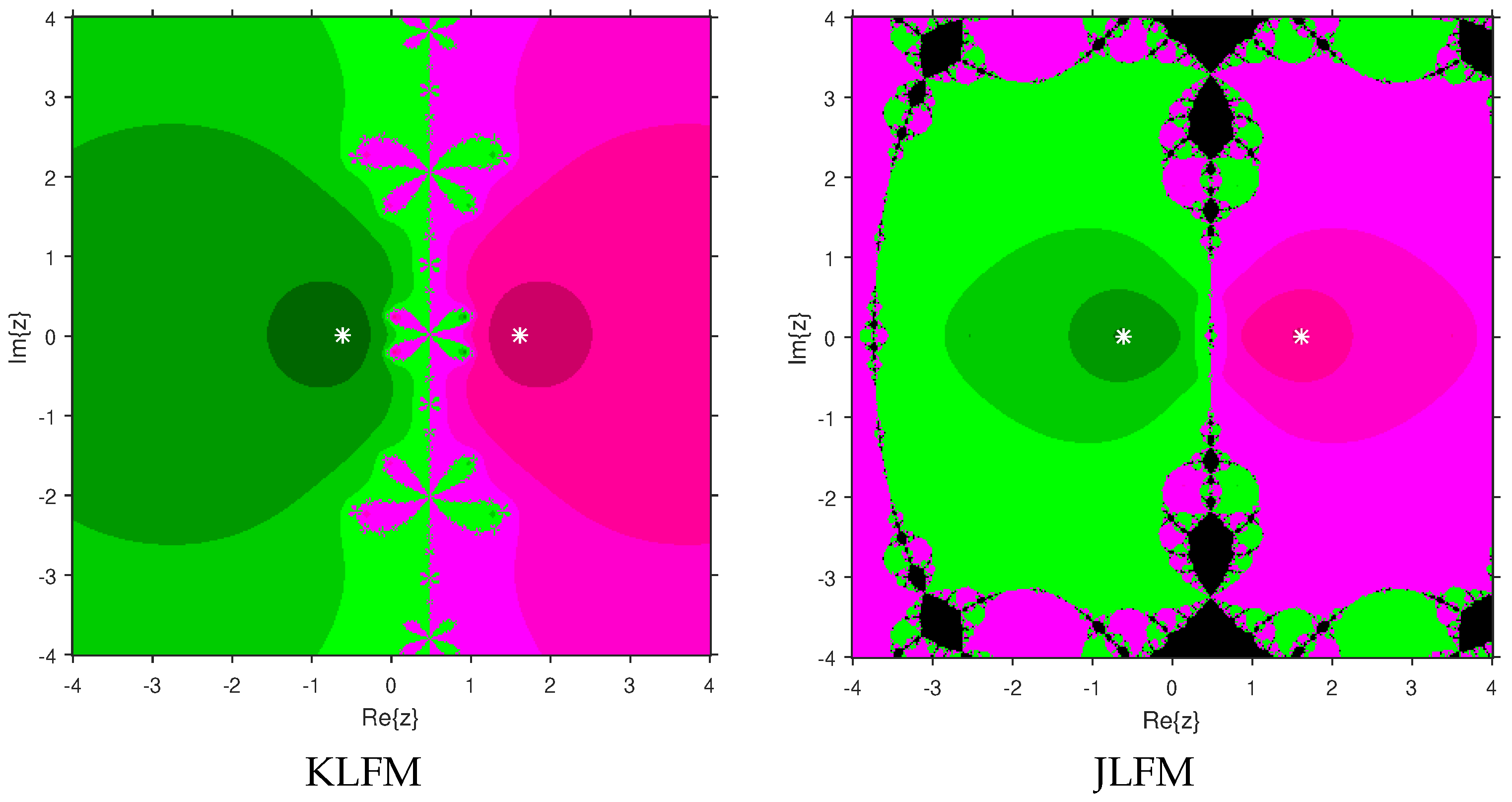
3. Comparison of Attraction Basins

The dynamical qualities of KLFM and JLFM were compared by analyzing the attraction basins for these methods. For generating the basins, these methods were applied to various complex polynomials W k ( z ) , k = 1 , 2 , , 10 , of degrees more than or equal to two. A region Z = [ 4 , 4 ] × [ 4 , 4 ] on C was selected with a grid of 400 × 400 points. Then, these methods were applied to find solutions of the considered polynomials W k ( z ) , where each point z 0 Z was engaged as a stater. If the point z 0 belonged to the set { z 0 C : z j z * a s j } , then it remained in the basin of a zero z * of a considered polynomial. We represent this z 0 with a distinct color related to z * . We assigned the light to dark colors to each z 0 as per the number of iterations. Non-convergence zones are displayed in black. We use the accuracy z j z * < 10 6 or executed 100 iterations for terminating the process. The diagrams were designed in MATLAB 2019a.
We start by considering polynomials W 1 ( z ) = z 2 1 and W 2 ( z ) = z 2 z 1 of degree two. The results of the comparison between the attraction basins for KLFM and JLFM are displayed in Figure 1 and Figure 2. In Figure 1, green and pink areas indicate the attraction basins corresponding to the zeros 1 and 1, respectively, of W 1 ( z ) . The basins of the solutions 1 + 5 2 and 1 5 2 of W 2 ( z ) = 0 are shown in Figure 2 in pink and green, respectively. Figure 3 and Figure 4 offer the attraction basins for KLFM and JLFM associated with the zeros of W 3 ( z ) = z 3 + ( 0.7250 + 1.6500 i ) z 0.2750 1.6500 i and W 4 ( z ) = z 3 z . The basins for KLFM and JLFM associated with the zeros 1, 1.401440 + 0.915201 i and 0.4014403 0.915201 i of W 3 ( z ) are given in Figure 3 using green, pink and blue, respectively. In Figure 4, the basins of the solutions 0, 1 and 1 of W 4 ( z ) = 0 are yellow, magenta and cyan, respectively. Next, we used polynomials W 5 ( z ) = z 4 10 z 2 + 9 and W 6 ( z ) = z 4 z of degree four to compare the attraction basins for KLFM and JLFM. The basins for KLFM and JLFM corresponding to the zeros 1 , 3, 3 and 1 of W 5 ( z ) are demonstrated in Figure 5 using yellow, pink, green and blue, respectively. Figure 6 provides the comparison of basins for these schemes associated with the solutions 0, 1, 1 2 3 2 i and 1 2 + 3 2 i of W 6 ( z ) = 0 , which are denoted in green, blue, yellow and red regions, respectively. Moreover, we selected polynomials W 7 ( z ) = z 5 + z and W 8 ( z ) = z 5 5 z 3 + 4 z of degree five to design and compare the attraction basins for KLFM and JLFM. In Figure 7, green, cyan, red, pink and yellow regions illustrate the attraction basins of the solutions 0.707106 0.707106 i , 0.707106 + 0.707106 i , 0.707106 + 0.707106 i , 0.707106 0.707106 i and 0, respectively, of W 7 ( z ) = 0 . Figure 8 gives the basins of zeros 0, 2, 1 , 2 and 1 of W 8 ( z ) in yellow, magenta, red, green and cyan, respectively. Lastly, sixth-degree complex polynomials W 9 ( z ) = z 6 + z 1 and W 10 ( z ) = z 6 0.5 z 5 + 11 4 ( 1 + i ) z 4 1 4 ( 19 + 3 i ) z 3 + 1 4 ( 11 + i ) z 2 1 4 ( 19 + 3 i ) z + 3 2 3 i are considered. In Figure 9, green, pink, red, yellow, cyan and blue colors illustrate the basins in relation to the solutions 1.134724 , 0.629372 0.735755 i , 0.7780895 , 0.451055 1.002364 i , 0.629372 + 0.735755 i and 0.451055 + 1.002364 i of W 9 ( z ) = 0 , respectively. In Figure 10, the attraction basins for KLFM and JLFM corresponding to the zeros 1 i , 1 2 i 2 , 3 2 i , 1, i and 1 + 2 i of W 10 ( z ) are given in blue, yellow, green, magenta, cyan and red, respectively.
From Figure 1, Figure 2, Figure 3, Figure 4, Figure 5, Figure 6, Figure 7, Figure 8, Figure 9 and Figure 10, we can deduce that KLFM has the wider basins in comparison to JLFM. It can be seen that the black zones that appear in Figure 1, Figure 5 and Figure 8 only appear for the JLFM and not the KLFM. Furthermore, the KLFM is better than the JLFM in terms of less chaotic behavior, as it can be seen that basins are bigger with the KLFM, and there are fewer changes of basin than for the JLFM in each figure, which means that the fractal dimension is smaller in KLFM, and consequently less chaotic. Hence, the overall conclusion of this comparison is that the numerical stability of KLFM is higher than that of JLFM. This means that KLFM is the preferred option for solving real problems. Moreover, in relation to the patterns that appear in the basin of attraction, it is clear that the KLFM is similar to third-order methods such us Halley or Chebyshev methods, and the immediate basin of attraction is big, and black zones are avoided. On the other hand, in the JLFM, everything seems more independent with different structures; for example, see Figure 9, where the roots are bounded by a small basin, and then a really big one in red appears in Figure 1, Figure 5 and Figure 8, where zones with no convergence appear, especially in Figure 5 where almost the half of the plane is black. Finally, in Figure 4, Figure 6, Figure 7 and Figure 9, it seems that compactification appears in the roots, but one of the basins is much bigger than the rest, and this behavior is really interesting and could be considered in the future.

4. Numerical Examples

A comparison of the radii of convergence balls is presented in this section. By applying the newly suggested theorems, the radii of KLFM and JLFM were obtained and compared for three numerical problems.
Example 1.
Let M = R and T = [ 1 , 1 ] . Consider F on T defined by
F ( q ) = e q 1 .
Using this definition, we have F ( q ) = e q and the solution q * = 0 . In order to verify the conditions ( C ) , we see that since F ( q * ) = 1 ,
| f ( q * ) 1 ( F ( v ) F ( q * ) ) | = | e v 1 | 1 + 1 2 2 ! + + 1 n ! 1 | v 0 | , | f ( q * ) 1 ( F ( u ) F ( z ) ) | = | e u e z | e ξ | u z | , ξ = 1 e 1 , | F ( q * ) 1 F ( z ) | = e z e 1 1 e 2 ,
since
T 0 = [ 1 , 1 ] B 0 , 1 e 1 = B 0 , 1 e 1 .
Hence, we can choose
w 0 ( t ) = ( e 1 ) t , w ( t ) = e 1 e 1 t and w 1 ( t ) = 2 .
Using Theorem 1 and Theorem 2, the values of d ˜ (for δ = 2 ) and d ¯ were calculated and are presented in Table 1.
Example 2.
Let M = R and T = [ 1 , 1 ] . Define F on T by
F ( q ) = sin ( q ) .
Using this definition, we have q * = 0 , such that F ( q ) = cos ( q ) :
| F ( q * ) 1 ( F ( v ) F ( q * ) ) | = | sin ( ξ ) | | v 0 | 1 | v 0 | , | F ( q * ) 1 ( F ( u ) F ( z ) ) | = | sin ( ξ ) | | u z | 1 | u z | , | F ( q * ) 1 F ( z ) | = | cos ( z ) | 1 /
Hence, we can choose w 0 ( t ) = w ( t ) = w 1 ( t ) = 1 . Using Theorem 1 and Theorem 2, the values of d ˜ (for δ = 2 ) and d ¯ are calculated and presented in Table 2.
Example 3.
In the end, we address the motivational problem given in the first section. We have q * = 1 . Additionally, ω 0 ( t ) = ω ( t ) = 96.662907 t and ω 1 ( t ) = 2 . We applied Theorem 1 and Theorem 2 to compute values of d ˜ (for δ = 2 ) and d ¯ . These values are presented in Table 3.

5. Conclusions

We provided the ball analysis results for the KLFM and JLFM under the same set of conditions. To establish these results, the first derivative and generalized Lipschitz conditions were employed. In this way, the usefulness of these methods was improved. In addition, the convergence ball and dynamics comparison between these methods were presented. Based on the comparison results, it was derived that the stability of the KLFM is higher, and it is a much better method than the JLFM in terms of convergence ball and dynamical quality. Notice that although method (3) (JLFM) was studied on M, the same proofs can be given for F : D B 1 B 2 , where B 1 and B 2 are Banach spaces and D is open and convex. Hence, the earlier result also extends to hold for Banach space-valued equations. As you may have noticed, our methodology does not depend on the methods. Therefore, it can be used to extend the usage of other methods using inverses. That includes single and multistep methods. Our future research will include the study of implicit methods, such as the ones in [30,31,32] and other such methods along the same lines, since they provide better stability during data processing.

Author Contributions

Conceptualization, I.K.A., S.R., S.S. and H.Y.; methodology, I.K.A., S.R., S.S. and H.Y.; software, I.K.A., S.R., S.S. and H.Y.; validation, I.K.A. and S.R.; formal analysis, I.K.A., S.R., S.S. and H.Y.; investigation, I.K.A., S.R., S.S. and H.Y.; resources, I.K.A., S.R., S.S. and H.Y.; data curation, I.K.A., S.R., S.S. and H.Y.; writing—original draft preparation, I.K.A., S.R., S.S. and H.Y.; writing—review and editing, I.K.A., S.R., S.S. and H.Y.; visualization, I.K.A., S.R., S.S. and H.Y.; supervision, I.K.A., S.R., S.S. and H.Y.; project administration, I.K.A., S.R., S.S. and H.Y.; funding acquisition, I.K.A., S.R., S.S. and H.Y. All authors have read and agreed to the published version of the manuscript.

Funding

This research received no external funding.

Informed Consent Statement

Not applicable.

Data Availability Statement

Not applicable.

Conflicts of Interest

The authors declare no conflict of interest.

References

  1. Amat, S.; Busquier, S. Advances in Iterative Methods for Nonlinear Equations; Springer: Cham, Switzerland, 2016. [Google Scholar]
  2. Amat, S.; Busquier, S.; Plaza, S. Dynamics of the King and Jarratt iterations. Aequationes Math. 2005, 69, 212–223. [Google Scholar] [CrossRef]
  3. Argyros, I.K. The Theory and Applications of Iteration Methods, 2nd ed.; Engineering Series; CRC Press, Taylor and Francis Group: Boca Raton, FL, USA, 2022. [Google Scholar]
  4. Cordero, A.; Torregrosa, J.R. Variants of Newtons method using fifth-order quadrature formulas. Appl. Math. Comput. 2007, 190, 686–698. [Google Scholar]
  5. Ezquerro, J.A.; Gutiérrez, J.M.; Hernández, M.A.; Salanova, M.A. Chebyshev-like methods and quadratic equations. Rev. Anal. Numer. Théor. Approx. 1999, 28, 23–35. [Google Scholar]
  6. Hueso, J.L.; Martínez, E.; Teruel, C. Convergence, efficiency and dynamics of new fourth and sixth order families of iterative methods for nonlinear systems. J. Comput. Appl. Math. 2015, 275, 412–420. [Google Scholar] [CrossRef]
  7. Petković, M.S.; Neta, B.; Petković, L.; Džunixcx, D. Multipoint Methods for Solving Nonlinear Equations; Elsevier: Amsterdam, The Netherlands, 2013. [Google Scholar]
  8. Rheinboldt, W.C. An adaptive continuation process for solving systems of nonlinear equations. In Mathematical Models and Numerical Methods; Tikhonov, A.N., Ed.; Instytut Matematyczny Polskiej Akademi Nauk: Warsaw, Poland, 1978; Volume 3, pp. 129–142. [Google Scholar]
  9. Traub, J.F. Iterative Methods for Solution of Equations; Prentice-Hall: Upper Saddle River, NJ, USA, 1964. [Google Scholar]
  10. Chun, C. Some variants of King’s fourth-order family of methods for nonlinear equations. Appl. Math. Comput. 2007, 190, 57–62. [Google Scholar] [CrossRef]
  11. King, J.F. A family of fourth-order methods for nonlinear equations. SIAM J. Numer. Anal. 1973, 10, 876–879. [Google Scholar] [CrossRef]
  12. Wang, X.; Kou, J.; Li, Y. Modified Jarratt method with sixth-order convergence. Appl. Math. Lett. 2009, 22, 1798–1802. [Google Scholar] [CrossRef] [Green Version]
  13. Jarratt, P. Some fourth order multipoint iterative methods for solving equations. Math. Comp. 1966, 20, 434–437. [Google Scholar] [CrossRef]
  14. Ghanbari, B. A new general fourth-order family of methods for finding simple roots of nonlinear equations. J. King Saud Univ.-Sci. 2011, 23, 395–398. [Google Scholar] [CrossRef] [Green Version]
  15. Grau-Sánchez, M.; Gutiérrez, J.M. Zero-finder methods derived from Obreshkovs techniques. Appl. Math. Comput. 2009, 215, 2992–3001. [Google Scholar]
  16. Cordero, A.; Hueso, J.L.; Martínez, E.; Torregrosa, J.R. A modified Newton–Jarratt’s composition. Numer. Algorithms 2010, 55, 87–99. [Google Scholar] [CrossRef]
  17. Sharma, J.R.; Guna, R.K.; Sharma, R. An efficient fourth order weighted-Newton method for systems of nonlinear equations. Numer. Algorithms 2013, 62, 307–323. [Google Scholar] [CrossRef]
  18. Sharma, J.R.; Arora, H. Efficient Jarratt-like methods for solving systems of nonlinear equations. Calcolo 2014, 51, 193–210. [Google Scholar] [CrossRef]
  19. Cordero, A.; García-Maimó, J.; Torregrosa, J.R.; Vassileva, M.P. Solving nonlinear problems by Ostrowski-Chun type parametric families. J. Math. Chem. 2015, 53, 430–449. [Google Scholar] [CrossRef] [Green Version]
  20. Solaiman, O.S.; Karim, S.A.A.; Hashim, I. Optimal fourth- and eighth-order of convergence derivative-free modifications of King’s method. J. King Saud Univ.-Sci. 2019, 31, 1499–1504. [Google Scholar] [CrossRef]
  21. Blanchard, P. Complex Analytic Dynamics on the Riemann Sphere. Bull. Am. Math. Soc. 1984, 11, 85–141. [Google Scholar] [CrossRef] [Green Version]
  22. Chen, D. On the convergence and optimal error estimates of King’s iteration procedures for solving nonlinear equations. Int. J. Comput. Math. 1989, 26, 229–237. [Google Scholar] [CrossRef]
  23. Hernández, M.A.; Salanova, M.A. Relaxing convergence conditions for the Jarratt method. Southwest J. Pure Appl. Math. 1997, 2, 16–19. [Google Scholar]
  24. Kou, J.; Li, Y. An improvement of the Jarratt method. Appl. Math. Comput. 2007, 189, 1816–1821. [Google Scholar] [CrossRef]
  25. Magreñán, Á.A. Different anomalies in a Jarratt family of iterative root-finding methods. Appl. Math. Comput. 2014, 233, 29–38. [Google Scholar]
  26. Neta, B.; Scott, M.; Chun, C. Basins of attraction for several methods to find simple roots of nonlinear equations. Appl. Math. Comput. 2012, 218, 10548–10556. [Google Scholar] [CrossRef]
  27. Regmi, S.; Argyros, I.K.; George, S.; Argyros, C.I. On the local convergence and comparison between two novel eighth convergence order schemes for solving nonlinear equations. Nonlinear Stud. 2021, 28, 1107–1116. [Google Scholar]
  28. Sharma, D.; Parhi, S.K.; Sunanda, S.K. Extending the convergence domain of deformed Halley method under ω condition in Banach spaces. Bol. Soc. Mat. Mex. 2021, 27, 32. [Google Scholar] [CrossRef]
  29. Sharma, D.; Parhi, S.K. On the local convergence of higher order methods in Banach spaces. Fixed Point Theory 2021, 22, 855–870. [Google Scholar] [CrossRef]
  30. Xu, Y.; Jiao, Y.; Chen, Z. On an independent subharmonic sequence for vibration isolation and suppression in a nonlinear rotor system. Mech. Syst. Signal Process. 2022, 178, 109259. [Google Scholar] [CrossRef]
  31. Xu, Y.; Chen, Z.; Luo, A. On bifurcation trees of period-1 to period-2 motions in a nonlinear Jeffcott rotor system. Int. J. Mech. Sci. 2019, 160, 429–450. [Google Scholar] [CrossRef]
  32. Xu, Y.; Chen, Z.; Luo, A. Period-1 Motion to Chaos in a Nonlinear Flexible Rotor System. Int. J. Bifurc. Chaos 2020, 30, 2050077. [Google Scholar] [CrossRef]
  33. Argyros, I.K. Unified convergence criteria for iterative Banach space valued methods with applications. Mathematics 2021, 9, 1942. [Google Scholar] [CrossRef]
Figure 1. Attraction basins comparison between KLFM and JLFM in relation to W 1 ( z ) .
Symmetry 14 02206 g001
Figure 2. Attraction basins comparison between KLFM and JLFM in relation to W 2 ( z ) .
Symmetry 14 02206 g002
Figure 3. Attraction basins comparison between KLFM and JLFM in relation to W 3 ( z ) .
Symmetry 14 02206 g003
Figure 4. Attraction basins comparison between KLFM and JLFM in relation to W 4 ( z ) .
Symmetry 14 02206 g004
Figure 5. Attraction basins comparison between KLFM and JLFM in relation to W 5 ( z ) .
Symmetry 14 02206 g005
Figure 6. Attraction basins comparison between KLFM and JLFM in relation to W 6 ( z ) .
Symmetry 14 02206 g006
Figure 7. Attraction basins comparison between KLFM and JLFM in relation to W 7 ( z ) .
Symmetry 14 02206 g007
Figure 8. Attraction basins comparison between KLFM and JLFM in relation to W 8 ( z ) .
Symmetry 14 02206 g008
Figure 9. Attraction basins comparison between KLFM and JLFM in relation to W 9 ( z ) .
Symmetry 14 02206 g009
Figure 10. Attraction basins comparison between KLFM and JLFM in relation to W 10 ( z ) .
Symmetry 14 02206 g010
Table 1. Comparison of convergence radii for Example 1.
KLFMJLFM
d 1 = 0.382692 d ¯ 1 = 0.382692
d 2 = 0.130790 d ¯ 2 = 0.114125
d ˜ = 0.130790 d ¯ = 0.114125
Table 2. Comparison of convergence radii for Example 2.
KLFMJLFM
d 1 = 0.666667 d ¯ 1 = 0.666667
d 2 = 0.318305 d ¯ 2 = 0.243217
d ˜ = 0.318305 d ¯ = 0.243217
Table 3. Comparison of convergence radii for Example 3.
KLFMJLFM
d 1 = 0.006897 d ¯ 1 = 0.006897
d 2 = 0.002379 d ¯ 2 = 0.002039
d ˜ = 0.002379 d ¯ = 0.002039
Publisher’s Note: MDPI stays neutral with regard to jurisdictional claims in published maps and institutional affiliations.

