Article

A Study of the Higgs Mass with the Effective Potential and Higgs Decays in the U(1)XSSM

1
Department of Physics, Hebei University, Baoding 071002, China
2
Key Laboratory of High-Precision Computation and Application of Quantum Field Theory of Hebei Province, Baoding 071002, China
3
Department of Physics, Chongqing University, Chongqing 401331, China
*
Author to whom correspondence should be addressed.
Symmetry 2022, 14(10), 2153; https://doi.org/10.3390/sym14102153
Submission received: 16 September 2022 / Revised: 8 October 2022 / Accepted: 11 October 2022 / Published: 14 October 2022
(This article belongs to the Special Issue Supersymmetry with Higgs Bosons Research)

Abstract

:
As the U(1) extension of the minimal supersymmetric standard model, the U ( 1 ) X SSM has new superfields, such as right-handed neutrinos, and three Higgs singlets. In the U ( 1 ) X SSM, the lightest CP-even Higgs mass m h 0 is studied by using the Higgs effective potential with one-loop corrections. We also calculate the Higgs decays h 0 γ γ , h 0 V V ( V = W , Z ) , h 0 l l ¯ Z , and h 0 ν ν ¯ Z . The obtained results are reasonable, and they are in favor of the study of the Higgs characteristic and the phenomenology of the U ( 1 ) X SSM.
PACS:
11.30.Er; 12.60.Jv; 14.80.Cp

1. Introduction

In the standard model (SM) of particle physics, the Higgs boson is the last particle to have been discovered, and it is inherently related to the mechanism of spontaneous symmetry breaking (SSB). The observation of the Higgs boson in 2012 [1,2] was a great success for the SM. Nevertheless, more detailed and precise investigations of the Higgs boson are required, and the search for a new physics beyond the SM is one of the major issues of particle physics. On the other hand, the SM has some shortcomings, such as its inability to explain neutrino mass and mixing [3,4], its inability to provide candidates for cold dark matter, its inability to explain the asymmetry of matter and antimatter in the universe, etc.
A famous extension of the SM is the minimal supersymmetric extension of the standard model (MSSM) [5,6], which has been researched by physicists for several decades. People have also extended the MSSM into multiple models, of which the U(1) extensions of MSSM are interesting. The U ( 1 ) X extension of the MSSM is called the U ( 1 ) X SSM [7,8,9] with the local gauge group S U ( 3 ) C × S U ( 2 ) L × U ( 1 ) Y × U ( 1 ) X . The U ( 1 ) X SSM has more superfields (three Higgs singlets and right-handed neutrinos) than the MSSM. The additional right-handed neutrinos can not only explain the tiny mass of the neutrino, but also provide a new dark matter candidate—the light sneutrino. The μ problem appearing in the MSSM is relieved in the U ( 1 ) X SSM by the terms μ H ^ u H ^ d and λ H S ^ H ^ u H ^ d , which produce an effective μ e f f = μ + λ H v S / 2 . The Higgs singlet S has a non-zero VEV ( v S / 2 ). The mixing of the CP-even parts of H d , H u , η , η ¯ , S can improve the lightest CP-even Higgs mass at the tree level.
Higgs pairs can be produced through gluon–gluon fusion [10,11] in pp collisions through loop diagrams. The Higgs boson mass and decays, including h 0 γ γ and h 0 V V ( with V = Z , W ) , have been studied in several models, such as the MSSM, NMSSM [12], B-LSSM [13], BLMSSM [14], and so on. In the U ( 1 ) X SSM, we study the lightest CP-even Higgs mass through the Higgs effective potential with one-loop corrections. The Higgs boson decays h 0 γ γ , h 0 V V ( with V = Z , W ) , h 0 l l ¯ Z , and h 0 ν l ν ¯ l Z ( with l = e , μ , τ ) are all calculated in this work.
For the decays h 0 to γ γ , Z Z , and W W , the current values of the corresponding ratios R γ γ , R Z Z , R W W are, respectively, R γ γ = 1.10 ± 0.07 , R W W = 1.19 ± 0.12 and R Z Z = 1.01 ± 0.07 [15]. R X X is a ratio that is defined as
R X X = Γ U ( 1 ) X ( h 0 g g ) Γ U ( 1 ) X ( h 0 X X ) Γ S M ( h 0 g g ) Γ S M ( h 0 X X ) .
The Higgs boson decays h 0 l l ¯ Z and h 0 ν l ν ¯ l Z ( with l = e , μ , τ ) [16] are within the reachable region of the LHC. Some future experiments that will include two circular lepton colliders (CEPC and FCC-ee) [17] and a linear lepton collider (ILC) have been proposed in order to study the properties of the Higgs boson. The accuracy of these colliders in measuring the Higgs boson decays will be clearly improved, and we believe that the decays h 0 l l ¯ Z and h 0 ν l ν ¯ l Z ( with l = e , μ , τ ) can be detected in the near future.
In Section 2, we briefly introduce the main content of the U ( 1 ) X SSM and its superfields. The formulations for the Higgs effective potential and Higgs boson decays h 0 γ γ ( W W , Z Z ) , h 0 l l ¯ Z , and h 0 ν l ν ¯ l Z ( with l = e , μ , τ ) are shown in Section 3. We analyze the results numerically in Section 4 and obtain a reasonable parameter space. The last section is used for the discussion and conclusion.

2. The Main Content of the U ( 1 ) X SSM

We extend the MSSM with the local gauge group U ( 1 ) X to obtain the U ( 1 ) X SSM, which has new superfields: three generations of right-handed neutrinos and three Higgs singlets. Then, the U ( 1 ) X SSM can account for the data of the neutrino oscillation. The introduction of three Higgs singlets ( η , η ¯ , and S) leads to the extension of the mass-squared matrix for CP-even Higgs. The new mixing of Higgs can improve the lightest CP-even Higgs mass at the tree level. One can find the particle contents in [8,18].
In the U ( 1 ) X SSM, the superpotential and soft SUSY breaking terms are shown [8,9,18]:
W = l W S ^ + μ H ^ u H ^ d + M S S ^ S ^ Y d d ^ q ^ H ^ d Y e e ^ l ^ H ^ d + λ H S ^ H ^ u H ^ d + λ C S ^ η ^ η ¯ ^ + κ 3 S ^ S ^ S ^ + Y u u ^ q ^ H ^ u + Y X ν ^ η ¯ ^ ν ^ + Y ν ν ^ l ^ H ^ u .
L s o f t = L s o f t M S S M B S S 2 L S S T κ 3 S 3 T λ C S η η ¯ + ϵ i j T λ H S H d i H u j T X I J η ¯ ν ˜ R I ν ˜ R J + ϵ i j T ν I J H u i ν ˜ R I l ˜ j J m η 2 | η | 2 m η ¯ 2 | η ¯ | 2 m S 2 S 2 ( m ν ˜ R 2 ) I J ν ˜ R I ν ˜ R J 1 2 M S λ X ˜ 2 + 2 M B B λ B ˜ λ X ˜ + h . c .
The two Higgs doublets and three Higgs singlets are
H u = H u + 1 2 v u + ϕ u + i P u 0 , H d = 1 2 v d + ϕ d + i P d 0 H d , η = 1 2 v η + ϕ η + i P η 0 , η ¯ = 1 2 v η ¯ + ϕ η ¯ + i P η ¯ 0 , S = 1 2 v S + ϕ s + i P s 0 .
v u , v d , v η , v η ¯ , and v S , respectively, represent the VEVs of the Higgs superfields H u , H d , η , η ¯ , and S. The definitions of the two angles are tan β = v u / v d and tan β η = v η ¯ / v η .
Y Y denotes the U ( 1 ) Y charge and Y X represents the U ( 1 ) X charge. One can write the covariant derivatives of the U ( 1 ) X SSM in the form
D μ = μ i Y , X g Y , g Y X g X Y , g X A μ Y A μ X ,
where A μ Y and A μ X denote the gauge fields of U ( 1 ) Y and U ( 1 ) X , respectively.
It is convenient to perform a change in the basis with the rotation matrix R [19,20]:
D μ = μ i Y Y , Y X g Y , g Y X g X Y , g X R T R A μ Y A μ X ,
g Y , g Y X g X Y , g X R T = g 1 , g Y X 0 , g X , R A μ Y A μ X = A μ Y A μ X .
In the end, the covariant derivatives of the U ( 1 ) X SSM turn into
D μ = μ i Y Y , Y X g 1 , g Y X 0 , g X A μ Y A μ X .
In the U ( 1 ) X SSM, the gauge bosons A μ X , A μ Y , and V μ 3 mix together at the tree level. We deduce their mass eigenvalues as
m γ 2 = 0 , m Z , Z 2 = 1 8 ( ( g 1 2 + g 2 2 + ( g Y X + g X ) 2 ) v 2 + 4 g X 2 ξ 2 ( g 1 2 + g 2 2 + ( g Y X + g X ) 2 ) 2 v 4 + 8 ( ( g Y X + g X ) 2 g 1 2 g 2 2 ) g X 2 v 2 ξ 2 + 16 g X 4 ξ 4 ) .
with v 2 = v u 2 + v d 2 and ξ 2 = v η 2 + v η ¯ 2 . Two mixing angles θ W and θ W [9,18] are used here.
Supposing μ , λ H , λ C , l W , M S , B μ , L S , T κ , T λ C , T λ H , κ , B S as real parameters, we show the simplified Higgs potential at the tree level [8]:
V 0 = 1 2 g X ( g X + g Y X ) ( | H d 0 | 2 | H u 0 | 2 ) ( | η | 2 | η ¯ | 2 ) + λ H 2 | H u 0 H d 0 | 2 + m S 2 | S | 2 + l W 2 + 1 8 g 1 2 + g 2 2 + ( g X + g Y X ) 2 ( | H d 0 | 2 | H u 0 | 2 ) 2 + 1 2 g X 2 ( | η | 2 | η ¯ | 2 ) 2 + λ C 2 | η η ¯ | 2 + ( μ 2 + λ H 2 | S | 2 + 2 Re [ μ λ H S ] ) ( | H d 0 | 2 + | H u 0 | 2 ) + λ C 2 | S | 2 ( | η | 2 + | η ¯ | 2 ) + m η 2 | η | 2 + 2 Re [ ( l W + 2 M S S ) ( λ C η η ¯ λ H H u 0 H d 0 + κ S 2 ) ] + 4 M S 2 | S | 2 + κ 2 | S | 4 + m η ¯ 2 | η ¯ | 2 + 2 Re [ λ C κ η η ¯ S 2 + 2 l W M S S λ C λ H η η ¯ H u 0 H d 0 ] + m H u 0 2 | H u | 2 + m H d 2 | H d | 2 + 2 Re L S S H d 0 H u 0 B μ + λ H κ ( S 2 ) + T λ H S + 1 3 T k S 3 + T λ C η η ¯ S + B S S 2 .
The corresponding tadpole equations at the tree level were also obtained in [8]. The tree-level mass-squared matrix for the CP-even Higgs ( ϕ d , ϕ u , ϕ η , ϕ η ¯ , ϕ s ) is
M h , t r e e 2 = m ϕ d ϕ d m ϕ u ϕ d m ϕ η ϕ d m ϕ η ¯ ϕ d m ϕ s ϕ d m ϕ d ϕ u m ϕ u ϕ u m ϕ η ϕ u m ϕ η ¯ ϕ u m ϕ s ϕ u m ϕ d ϕ η m ϕ u ϕ η m ϕ η ϕ η m ϕ η ¯ ϕ η m ϕ s ϕ η m ϕ d ϕ η ¯ m ϕ u ϕ η ¯ m ϕ η ϕ η ¯ m ϕ η ¯ ϕ η ¯ m ϕ s ϕ η ¯ m ϕ d ϕ s m ϕ u ϕ s m ϕ η ϕ s m ϕ η ¯ ϕ s m ϕ s ϕ s ,
m ϕ d ϕ d = m H d 2 + μ 2 + 1 8 ( [ g 1 2 + ( g X + g Y X ) 2 + g 2 2 ] ( 3 v d 2 v u 2 ) + 2 ( g Y X g X + g X 2 ) ( v η 2 v η ¯ 2 ) ) + 2 v S μ λ H + 1 2 ( v u 2 + v S 2 ) λ H 2 ,
m ϕ d ϕ u = 1 4 g 2 2 + ( g Y X + g X ) 2 + g 1 2 v d v u + λ H 2 v d v u λ H l W 1 2 λ H ( v η v η ¯ λ C + v S 2 κ ) B μ 2 v S ( 1 2 T λ H + M S λ H ) ,
m ϕ u ϕ u = m H u 2 + μ 2 + 1 8 ( [ g 1 2 + ( g X + g Y X ) 2 + g 2 2 ] ( 3 v u 2 v d 2 ) + 2 ( g Y X g X + g X 2 ) ( v η ¯ 2 v η 2 ) ) + 2 v S μ λ H + 1 2 ( v d 2 + v S 2 ) λ H 2 ,
m ϕ d ϕ η = 1 2 g X ( g Y X + g X ) v d v η 1 2 v u v η ¯ λ H λ C ,
m ϕ u ϕ η = 1 2 g X ( g Y X + g X ) v u v η 1 2 v d v η ¯ λ H λ C ,
m ϕ η ϕ η = m η 2 + 1 4 ( g Y X g X + g X 2 ) ( v d 2 v u 2 ) + 2 g X 2 ( 3 v η 2 v η ¯ 2 ) + λ C 2 2 ( v η ¯ 2 + v S 2 ) ,
m ϕ d ϕ η ¯ = 1 2 g X ( g Y X + g X ) v d v η ¯ 1 2 v u v η λ H λ C ,
m ϕ u ϕ η ¯ = 1 2 g X ( g Y X + g X ) v u v η ¯ 1 2 v d v η λ H λ C ,
m ϕ η ϕ η ¯ = ( λ C 2 g X 2 ) v η v η ¯ + λ C 2 ( 2 l W λ H v d v u ) + v S 2 ( 2 M S λ C + T λ C ) + v S 2 2 λ C κ ,
m ϕ η ¯ ϕ η ¯ = m η ¯ 2 + 1 4 ( g Y X g X + g X 2 ) ( v u 2 v d 2 ) + 2 g X 2 ( 3 v η ¯ 2 v η 2 ) + λ C 2 2 v η 2 + v S 2 ,
m ϕ d ϕ s = λ H v d v S + 2 v d μ v u ( κ v S + 2 M S ) λ H 1 2 v u T λ H ,
m ϕ u ϕ s = λ H v u v S + 2 v u μ v d ( κ v S + 2 M S ) λ H 1 2 v d T λ H ,
m ϕ η ϕ s = λ C v η v S + v η ¯ ( κ v S + 2 M S ) λ C + 1 2 v η ¯ T λ C ,
m ϕ η ¯ ϕ s = λ C v η ¯ v S + v η ( κ v S + 2 M S ) λ C + 1 2 v η T λ C ,
m ϕ s ϕ s = m S 2 + 2 l W + 3 v S ( κ v S + 2 2 M S ) + λ C v η v η ¯ λ H v d v u κ + 2 B S + 1 2 λ C 2 ξ 2 + 1 2 λ H 2 v 2 + 4 M S 2 + 2 v S T κ .

3. Formulation

The one-loop effective potential can be written in the following form:
V e f f = V 0 + V 1 .
Here, V 1 is the potential from a one-loop correction. With the dimensional reduction and the DR renormalization scheme, the effective Higgs potential up to the one-loop correction is shown in the Landau gauge, and the concrete form of V 1 is [21,22,23]:
V 1 = i n i 64 π 2 m i 4 ( ϕ d , ϕ u , ϕ η , ϕ η ¯ , ϕ s ) log m i 2 ( ϕ d , ϕ u , ϕ η , ϕ η ¯ , ϕ s ) Q 2 3 2 .
We take the renormalization scale Q at the TeV order. The degrees of freedom for each mass eigenstate are represented by n i (−12 for quarks, −4 for leptons and charginos, −2 for neutralinos and neutrinos, 6 for squarks, 2 for sleptons and charged Higgs, 3 and 6 for Z ( Z ) and W bosons, and 1 for sneutrinos and the neutral Higgs scalars). The mass matrices are needed, and we collect the mass matrices of the CP-even sneutrino, CP-odd sneutrino, slepton, squark, chargino, and neutralino.
The mass matrix for the CP-even sneutrino ( ϕ l , ϕ r ) reads
M ν ˜ R 2 = m ϕ l ϕ l m ϕ r ϕ l T m ϕ l ϕ r m ϕ r ϕ r ,
m ϕ l ϕ l = 1 8 ( g 1 2 + g Y X 2 + g 2 2 + g Y X g X ) ( v d 2 v u 2 ) + 2 g Y X g X ( v η 2 v η ¯ 2 ) + v u 2 2 Y ν 2 + m L ˜ 2 , m ϕ l ϕ r = 1 2 v u T ν + v u v η ¯ Y X Y ν 1 2 v d ( λ H v S + 2 μ ) Y ν , m ϕ r ϕ r = 1 8 ( g Y X g X + g X 2 ) ( v d 2 v u 2 ) + 2 g X 2 ( v η 2 v η ¯ 2 ) + v η v S Y X λ C + m ν ˜ 2 + 1 2 v u 2 | Y ν | 2 + v η ¯ ( 2 v η ¯ Y X 2 + 2 T X ) .
To obtain the masses of sneutrinos, the rotation matrix Z R is used to diagonalize M ν ˜ R 2 .
We also deduce the mass matrix for a CP-odd sneutrino ( σ l , σ r ) :
M ν ˜ I 2 = m σ l σ l m σ r σ l T m σ l σ r m σ r σ r ,
m σ l σ l = 1 8 ( g 1 2 + g Y X 2 + g 2 2 + g Y X g X ) ( v d 2 v u 2 ) + 2 g Y X g X ( v η 2 v η ¯ 2 ) + v u 2 2 Y ν 2 + m L ˜ 2 , m σ l σ r = 1 2 v u T ν v u v η ¯ Y X Y ν 1 2 v d ( λ H v S + 2 μ ) Y ν , m σ r σ r = 1 8 ( g Y X g X + g X 2 ) ( v d 2 v u 2 ) + 2 g X 2 ( v η 2 v η ¯ 2 ) v η v S Y X λ C + m ν ˜ 2 + 1 2 v u 2 | Y ν | 2 + v η ¯ ( 2 v η ¯ Y X Y X 2 T X ) .
We use Z I to diagonalize the mass-squared matrix of the sneutrino M ν ˜ I 2 .
On the basis of ( e ˜ L , e ˜ R ) , the mass matrix for a slepton is shown and diagonalized by Z E through the formula Z E m e ˜ 2 Z E , = m 2 , e ˜ d i a g ,
m e ˜ 2 = m e ˜ L e ˜ L 1 2 2 v d T e v u ( λ H v S + 2 μ ) Y e 1 2 2 v d T e v u Y e ( 2 μ + v S λ H ) m e ˜ R e ˜ R .
m e ˜ L e ˜ L = m L ˜ 2 + 1 8 ( g 1 2 + g Y X 2 + g Y X g X g 2 2 ) ( v d 2 v u 2 ) + 2 g Y X g X ( v η 2 v η ¯ 2 ) + v d 2 2 Y e 2 , m e ˜ R e ˜ R = m E ˜ 2 1 8 ( [ 2 ( g 1 2 + g Y X 2 ) + 3 g Y X g X + g X 2 ] ( v d 2 v u 2 ) + ( 4 g Y X g X + 2 g X 2 ) ( v η 2 v η ¯ 2 ) ) + 1 2 v d 2 Y e 2 .
The mass-squared matrix for a down-type squark is shown on the basis of d ˜ L 0 , d ˜ R 0 :
M D ˜ 2 = m d ˜ L 0 d ˜ L 0 , m d ˜ R 0 d ˜ L 0 , m d ˜ L 0 d ˜ R 0 , m d ˜ R 0 d ˜ R 0 , ,
where
m d ˜ L 0 d ˜ L 0 , = 1 24 ( 3 g 2 2 + g 1 2 + g Y X 2 + g Y X g X ) ( v u 2 v d 2 ) + 2 g Y X g X ( v η ¯ 2 v η 2 ) + m Q ˜ 2 + v d 2 2 Y d 2 , m d ˜ L 0 d ˜ R 0 , = 1 2 2 ( v d T d + v u Y d μ ) + v u v S Y d λ H , m d ˜ R 0 d ˜ R 0 , = 1 24 ( 2 g 1 2 + 2 g Y X 2 + 5 g Y X g X + 3 g X 2 ) ( v u 2 v d 2 ) + 2 ( 2 g Y X g X + 3 g X 2 ) ( v η ¯ 2 v η 2 ) + m D ˜ 2 + v d 2 2 Y d 2 .
On the basis of u ˜ L 0 , u ˜ R 0 , the mass-squared matrix for an up-type squark is
M U ˜ 2 = m u ˜ L 0 u ˜ L 0 , m u ˜ R 0 u ˜ L 0 , m u ˜ L 0 u ˜ R 0 , m u ˜ R 0 u ˜ R 0 , ,
where
m u ˜ L 0 u ˜ L 0 , = 1 24 ( g 1 2 3 g 2 2 + g Y X 2 + g Y X g X ) ( v u 2 v d 2 ) + g Y X g X ( 2 v η ¯ 2 2 v η 2 ) + m Q ˜ 2 + v u 2 2 Y u 2 , m u ˜ L 0 u ˜ R 0 , = 1 2 2 ( v d Y u μ v u T u ) + v d v S Y u λ H , m u ˜ R 0 u ˜ R 0 , = 1 24 ( 4 g 1 2 + 4 g Y X 2 + 7 g Y X g X + 3 g X 2 ) ( v d 2 v u 2 ) + 2 ( 4 g Y X g X + 3 g X 2 ) ( v η 2 v η ¯ 2 ) + m U ˜ 2 + v u 2 2 Y u 2 .
On the basis of ( λ B ˜ , W ˜ 0 , H ˜ d 0 , H ˜ u 0 , λ X ˜ , η ˜ , η ¯ ˜ , s ˜ ) , the mass matrix for a neutralino is
m χ ˜ 0 = M 1 0 g 1 2 v d g 1 2 v u M B B 0 0 0 0 M 2 1 2 g 2 v d 1 2 g 2 v u 0 0 0 0 g 1 2 v d 1 2 g 2 v d 0 m H ˜ u 0 H ˜ d 0 m λ X ˜ H ˜ d 0 0 0 λ H v u 2 g 1 2 v u 1 2 g 2 v u m H ˜ d 0 H ˜ u 0 0 m λ X ˜ H ˜ u 0 0 0 λ H v d 2 M B B 0 m H ˜ d 0 λ X ˜ m H ˜ u 0 λ X ˜ M B L g X v η g X v η ¯ 0 0 0 0 0 g X v η 0 1 2 λ C v S 1 2 λ C v η ¯ 0 0 0 0 g X v η ¯ 1 2 λ C v S 0 1 2 λ C v η 0 0 λ H v u 2 λ H v d 2 0 1 2 λ C v η ¯ 1 2 λ C v η m s ˜ s ˜ ,
m H ˜ d 0 H ˜ u 0 = 1 2 λ H v S μ , m H ˜ d 0 λ X ˜ = 1 2 ( g Y X + g X ) v d , m H ˜ u 0 λ X ˜ = 1 2 ( g Y X + g X ) v u , m s ˜ s ˜ = 2 M S + 2 κ v S .
This matrix is diagonalized by Z N
Z N m χ ˜ 0 Z N = m χ ˜ 0 d i a g .
On the basis of W ˜ , H ˜ d , W ˜ + , H ˜ u + , the definition of the mass matrix for charginos is given by
M χ ˜ ± = M 2 1 2 g 2 v u 1 2 g 2 v d 1 2 λ H v S + μ .
This matrix is diagonalized by U and V:
U M χ ˜ ± V = M χ ˜ ± d i a g .
Here, we use the conditions at the one-loop level through the following formula:
V e f f ϕ u = V e f f ϕ d = V e f f ϕ η = V e f f ϕ η ¯ = V e f f ϕ s = 0 .
The corresponding analytic results are very tedious, and we resolve the equations numerically. In order to save space in the text, we do not show the tedious analytic results here.
The mass-squared matrix of the CP-even Higgs is corrected by one-loop contributions from the effective potential V e f f :
M h 2 = M h , t r e e 2 + Δ M h 2 .
The elements of the corrected mass-squared matrix M h , i j 2 can be deduced from the one-loop effective potential V e f f through the following formula:
M h , i j 2 = 2 V e f f ϕ i ϕ j | ϕ i , ϕ j = ϕ d , ϕ u , ϕ η , ϕ η ¯ , ϕ s .
The lightest eigenvalue of M h 2 should be the square of m h 0 125 GeV.
Gluon fusion ( g g h 0 ) [10,11] chiefly produces h 0 at the LHC. With large Yukawa coupling, the virtual t-quark loop is the dominant contribution in the one-loop diagrams. Large couplings of new particles can lead to considerable corrections:
Γ N P ( h 0 g g ) = G F α s 2 m h 0 3 64 2 π 3 | q g h 0 q q A 1 / 2 ( x q ) + q ˜ g h 0 q ˜ q ˜ m Z 2 m q ˜ 2 A 0 ( x q ˜ ) | 2 ,
with x a = m h 0 2 / ( 4 m a 2 ) . Here, q represents a quark, and q ˜ denotes a squark. The functions A 1 / 2 ( x ) and A 0 ( x ) are defined as
A 1 / 2 ( x ) = 2 x + ( x 1 ) g ( x ) / x 2 , A 0 ( x ) = g ( x ) x / x 2 ,
g ( x ) = arcsin 2 x , x 1 1 4 ln 1 + 1 1 / x 1 1 1 / x i π 2 , x > 1 .
The concrete expressions for g h 0 q q and g h 0 q ˜ q ˜ are
g h 0 q q = v m q C h 0 q q , g h 0 q ˜ q ˜ = S W C W e m Z C h 0 q ˜ q ˜ .
Here, S W = sin θ W and C W = cos θ W , with θ W denoting the Weinberg angle. The coupling constants C h 0 q q and C h 0 q ˜ q ˜ are defined as
L C h 0 q q ( h 0 q ¯ q ) + C h 0 q ˜ q ˜ ( h 0 q ˜ q ˜ ) ,
C h 0 d d = 1 2 Y d Z b , 1 H , C h 0 u u = 1 2 Y u Z b , 2 H .
The couplings of the CP-even Higgs with scalar quarks ( C h 0 D ˜ j D ˜ k and C h 0 U ˜ j U ˜ k ) are deduced as
C h 0 D ˜ j D ˜ k = 1 12 a = 1 3 { Z j a D , Z k a D ( 12 v d Y d , a 2 Z i 1 H + ( v d Z i 1 H v u Z i 2 H ) ( 3 g 2 2 + g Y X g X + g 1 2 + g Y X 2 ) + 2 g Y X g X ( v η Z i 3 H v η ¯ Z i 4 H ) ) + Z j 3 + a D , Z k 3 + a D ( 2 ( 2 g Y X g X + 3 g X 2 ) ( v η Z i 3 H v η ¯ Z i 4 H ) + ( 2 g 1 2 + 2 g Y X 2 + 3 g X 2 + 5 g Y X g X ) ( v d Z i 1 H v u Z i 2 H ) 12 v d Y d , a 2 Z i 1 H ) + 6 ( ( Z j a D , Z k 3 + a D + Z j 3 + a D , Z k a D ) [ Y d , a ( λ H v S Z i 2 H + 2 μ Z i 2 H + λ H v u Z i 5 H ) 2 Z i 1 H T d , a ] ) } ,
C h 0 U ˜ j U ˜ k = 1 12 a = 1 3 { Z j a U , Z k a U ( 12 v u Y u , a 2 Z i 2 H ( v d Z i 1 H v u Z i 2 H ) + ( g 1 2 3 g 2 2 + g Y X g X + g Y X 2 ) + 2 g Y X g X ( v η Z i 3 H v η ¯ Z i 4 H ) ) + Z j 3 + a U , Z k 3 + a U ( 2 ( 3 g X 2 + 4 g Y X g X ) ( v η ¯ Z i 4 H v η Z i 3 H ) + ( 3 g X 2 + 4 g 1 2 + 4 g Y X 2 + 7 g Y X g X ) ( v u Z i 2 H v d Z i 1 H ) 12 v u Y u , a 2 Z i 2 H ) + 6 ( ( Z j a U , Z k 3 + a U + Z j 3 + a U , Z k a U ) [ Y u , a ( 2 μ Z i 1 H + λ H v d Z i 5 H + λ H v S Z i 1 H ) 2 T u , a Z i 2 H ] ) ) } .
For the decay h 0 γ γ , the leading order contributions are from the one-loop diagrams. The decay width is written in the following form:
Γ U ( 1 ) X ( h 0 γ γ ) = G F α 2 m h 0 3 128 2 π 3 | f N c Q f 2 g h 0 f f A 1 / 2 ( x f ) + g h 0 H ± H ± m W 2 m H ± 2 A 0 ( x H ± ) + g h 0 W W A 1 ( x W ) + i = 1 2 g h 0 χ i ± χ i ± m W m χ i A 1 / 2 ( x χ i ) + f ˜ N c Q f 2 g h 0 f ˜ f ˜ m Z 2 m f ˜ 2 A 0 ( x f ˜ ) | 2 .
The function A 1 ( x ) is defined as
A 1 ( x ) = 2 x 2 + 3 x + 3 ( 2 x 1 ) g ( x ) / x 2 .
The relevant couplings are defined in the following form:
g h 0 W W = S W e m W C h 0 W W , g h 0 Z Z = C W S W e m Z C h 0 Z Z , g h 0 χ i ± χ i ± = 2 S W e C h 0 χ i ± χ i ± L , g h 0 H ± H ± = v 2 m W 2 C h 0 H ± H ± , g h 0 L ˜ L ˜ = S W C W e m Z C h 0 L ˜ L ˜ ,
L C h 0 W W g μ ν h 0 W μ W ν + C h 0 Z Z g μ ν h 0 Z μ Z ν + C h 0 L ˜ L ˜ h 0 L ˜ L ˜ + χ ¯ i ± ( C h 0 χ i ± χ j ± L P L + C h 0 χ i ± χ j ± R P R ) χ j ± h 0 + C h 0 H ± H ± h 0 H ± H ± .
The couplings for h 0 W W and h 0 Z Z are
C h 0 W W = 1 2 g 2 2 ( v d Z i 1 H + v u Z i 2 H ) , C h 0 Z Z = 1 2 ( [ g 1 cos θ W S W + g 2 C W cos θ W ( g Y X + g X ) sin θ W ] 2 × ( v d Z i 1 H + v u Z i 2 H ) + 4 g X 2 sin 2 θ W ( v η ¯ Z i 4 H + v η Z i 3 H ) ) .
Then, the CP-even Higgs–slepton–slepton coupling C h 0 L ˜ L ˜ reads as
C h 0 L ˜ n L ˜ m = 1 4 a = 1 3 { Z m , a E , Z n , a E ( ( g 2 2 g Y X g X g 1 2 g Y X 2 ) ( v d Z b 1 H v u Z b 2 H ) + g Y X g X ( v η ¯ Z b 4 H v η Z b 3 H ) ) + Z m , 3 + a E , Z n , 3 + a E ( ( 2 g 1 2 + 2 g Y X 2 + 3 g Y X g X + g X 2 ) ( v d Z b 1 H v u Z b 2 H ) + 2 ( g Y X g X + g X 2 ) ( v η Z b 3 H v η ¯ Z b 4 H ) ) + Z m , a E , Z n , 3 + a E + Z m , 3 + a E , Z n , a E × Y e , a 2 ( v S λ H + 2 μ ) Z b 2 H + 2 v u λ H Z b 5 H 2 2 T e , a Z b 1 H } .
The CP-even Higgs– H ± H ± coupling C h 0 H m ± H n ± is
C h 0 H m ± H n ± = 1 4 { ( Z b 2 H Z m 2 + Z b 1 H Z m 1 + ) ( [ ( g Y X + g X ) 2 + g 1 2 + g 2 2 ] ( v u Z n 2 + + v d Z n 1 + ) + ( g 2 2 2 λ H 2 ) ( v d Z n 1 + v u Z n 2 + ) ) + ( Z b 2 H Z m 1 + + Z b 1 H Z m 2 + ) ( [ ( g Y X + g X ) 2 2 g 2 2 + 2 λ H 2 + g 1 2 ] ( v u Z n 1 + + v d Z n 2 + ) ) 2 Z b 4 H ( Z m 2 + Z m 1 + ) ( ( g Y X g X + g X 2 ) v η ¯ ( Z n 2 + + Z n 1 + ) + λ c v η λ H × ( Z n 1 + Z n 2 + ) ) + Z b 3 H ( Z m 2 + + Z m 1 + ) ( g Y X g X + g X 2 ) ( v η Z n 1 + v η Z n 2 + ) + [ Z b 4 H λ c v η ¯ λ H + Z b 5 H 2 T λ , H + 2 λ H ( κ v s + 2 M S + 2 μ + λ H v S ) ] ( Z m 2 + + Z m 1 + ) ( Z n 2 + + Z n 1 + ) } .
We show the left-handed coupling of h 0 χ n ± χ m ± :
C h 0 χ n ± χ m ± L = 1 2 g 2 U m 1 V n 2 Z b 2 H + U m 2 ( g 2 V n 1 Z b 1 H + λ H V n 2 Z b 5 H ) .
The formulae for h 0 Z Z , W W are expressed as [24,25,26]:
Γ ( h 0 W W ) = 3 e 4 m h 0 512 π 3 S W 4 | g h 0 W W | 2 F ( m W m h 0 ) , Γ ( h 0 Z Z ) = e 4 m h 0 2048 π 3 S W 4 C W 4 | g h 0 Z Z | 2 7 40 3 S W 2 + 160 9 S W 4 F ( m Z m h 0 ) .
The concrete form of F ( x ) is
F ( x ) = ( 1 x 2 ) 47 2 x 2 13 2 + 1 x 2 3 ( 1 6 x 2 + 4 x 4 ) ln x + 3 ( 1 8 x 2 + 20 x 4 ) 4 x 2 1 cos 1 3 x 2 1 2 x 3 .
We also study the processes of h 0 l ¯ l Z and h 0 ν ¯ l ν l Z ( with l = e , μ , τ ) . The latter is simpler than the former and can be obtained by taking the limit m l 0 from the former, where m l denotes the mass of a lepton. For the processes of h 0 ( p 1 ) l ( p 2 ) + l ¯ ( p 3 ) + Z ( p 4 ) , the diagrams are shown in Figure 1.
The external particles all satisfy the on-shell condition: p 1 2 = m h 0 2 , p 2 2 = p 3 2 = m l 2 and p 4 2 = m Z 2 . We use the Mandelstam invariants: s = ( p 2 + p 3 ) 2 , t = ( p 3 + p 4 ) 2 , u = ( p 2 + p 4 ) 2 and s + t + u = m h 0 2 + 2 m l 2 + m Z 2 . In our calculation, all lepton masses and the couplings of l ¯ H 0 ( G 0 ) l are kept.
From the diagrams in Figure 1, we can obtain the decay width through the following formula [16]:
Γ ( h 0 l l ¯ Z ) = 1 256 π 3 m h 0 3 4 m l 2 ( m h 0 m Z ) 2 d s t t + | M | 2 .
Here, M is the Feynman amplitude for Figure 1. The definitions of t ± are
t ± = 1 2 m h 0 2 + 2 m l 2 + m Z 2 s ± 1 4 m l 2 s 1 / 2 ( m h 0 2 + m Z 2 s ) 2 4 m h 0 2 m Z 2 1 / 2 .

4. Numerical Results

To study the lightest CP-even Higgs h 0 mass ( m h 0 125 GeV) and h 0 decays h 0 V V ( with V = γ , W , Z ) , h 0 l l ¯ Z , and h 0 ν l ν ¯ l Z ( with l = e , μ , τ ) in the U ( 1 ) X SSM, we consider the mass constraint for the Z boson ( M Z > 5.1 TeV) [27] from LHC experiments. The constraints M Z / g X 6 TeV [28,29] and tan β η < 1.5 [30] are also taken into account. The parameters are used to make the scalar lepton masses larger than 700 GeV and the chargino masses larger than 1100 GeV [31].
Some parameters are adopted here with i = 1 , 2 , 3 :
κ = Y X i i = 1 , v S = 3.6 TeV , μ = M 1 = T d i i = 1 TeV , M S = 2.7 TeV , tan β η = 0.8 , B μ = B S = m L ˜ i i 2 = 1 TeV 2 , l W = 4 TeV 2 , l S = 300 TeV 3 , T κ = 1.6 TeV , M 2 = 1.2 TeV , M B L = 0.3 TeV , T X i i = T e i i = 0.5 TeV , T ν i i = 0.8 TeV , m E ˜ i i 2 = m D ˜ i i 2 = 5 TeV 2 , m ν ˜ i i 2 = 0.5 TeV 2 , ξ = 17 TeV .
To simplify the numerical discussion, we use the following relations:
T u i i = T u , m U ˜ i i 2 = M U 2 , m Q ˜ i i 2 = M Q 2 , ( i = 1 , 2 , 3 ) .
The parameters T u , m Q ˜ , and m U ˜ all emerge in the soft breaking terms and are included in L s o f t M S S M . T u is the coupling constant for the trilinear scalar coupling T u H u Q ˜ U ˜ . For the scalar quark fields Q ˜ and U ˜ , m Q ˜ and m U ˜ are, respectively, mass terms corresponding to m Q ˜ 2 Q ˜ Q ˜ and m U ˜ 2 U ˜ U ˜ .
To explore the parameter space better, we randomly scan the parameters as follows:
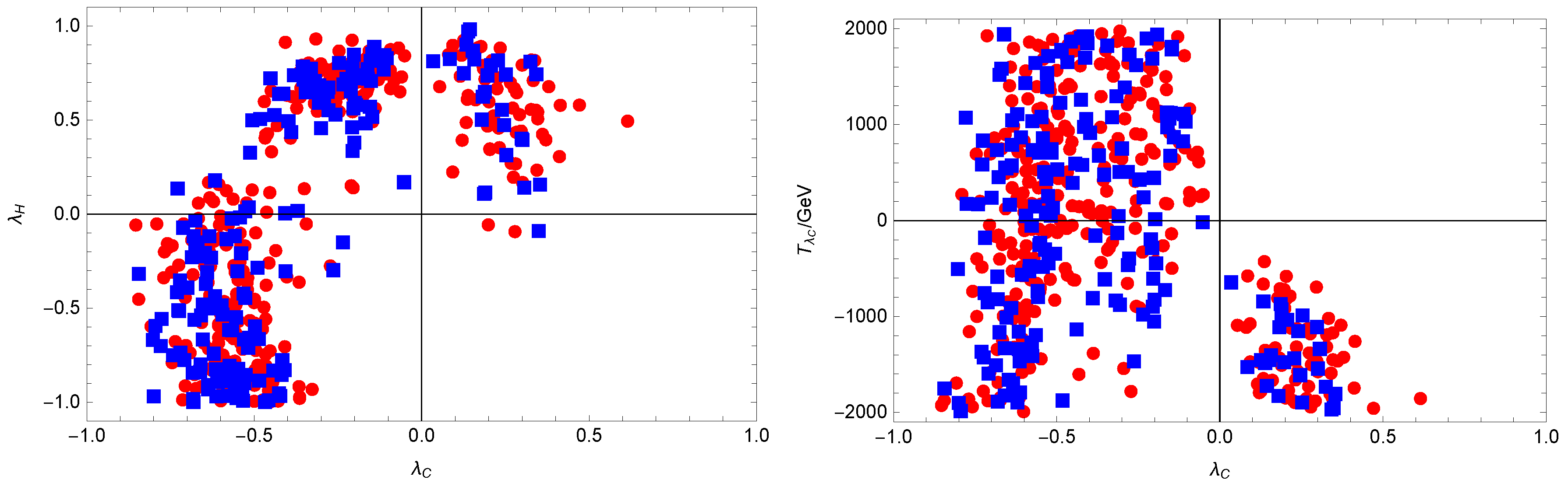
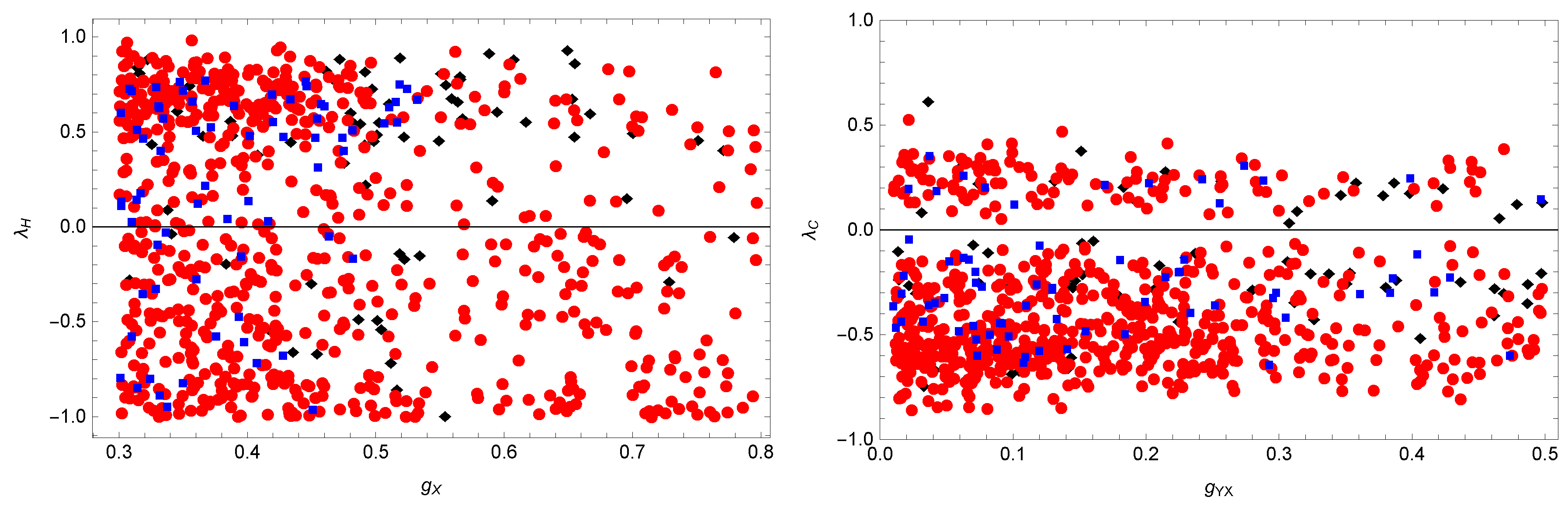
5 tan β 50 , 0.3 g X 0.8 , 0.01 g Y X 0.5 , 1 λ C 1 , 1 λ H 1 , 2 TeV T λ C 2 TeV , 2 TeV T λ H 2 TeV , 5 TeV T u 5 TeV , 4 TeV 2 M Q 2 8 TeV 2 , 4 TeV 2 M U 2 8 TeV 2 .
In Figure 2 and Figure 3, a 🟦 denotes the lightest CP-even Higgs mass in the region 123 GeV m h 0 127 GeV . A 🔴 represents the regions where 120 GeV m h 0 < 123 GeV and 127 GeV < m h 0 130 GeV . In the left diagram of Figure 2, the numerical results of m h 0 are plotted on the plane of g X versus g Y X . g X is the gauge coupling constant of the U ( 1 ) X group. g Y X is the mixing gauge coupling constant of the U ( 1 ) Y group and U ( 1 ) X group. So, they should have considerable effects on the results. Most of 🟦 and 🔴 are concentrated at the bottom left, forming a triangle with two sides as 0.3 g X 0.55 and 0 < g Y X 0.35 . The points are sparse in the other region. For the right diagram, we show the results of m h 0 in the plane of g X versus λ C . There are more points in the region where λ C < 0 than in the region where λ C > 0 . The concentrated area of 🟦 and 🔴 is like a rectangle with 0.1 λ C 0.6 and 0.3 g X 0.45 .
In the left diagram of Figure 3, m h 0 is shown on the plane of λ C versus λ H . Many points are in the first, second, and third quadrants. In the fourth quadrant, few points appear. This implies that the second and third quadrants are better for the 🟦. The numerical results of m h 0 versus λ C and T λ C are plotted in the right diagram of Figure 3. Obviously, the first quadrant is blank. That is to say, as λ C > 0 and T λ C > 0 , there is not any suitable result. Many 🟦 and 🔴 emerge in the second and third quadrants. In the fourth quadrant, the points are concentrated in the lower left corner. From Figure 2 and Figure 3, we can see that λ C , λ H , and T λ C are sensitive parameters for m h 0 .
The ratio R γ γ is also researched, and the corresponding results are shown in Figure 4 and Figure 5, where the notations are 🔴 0.95 R γ γ 1.03 and 🟦  1.03 < R γ γ 1.17 . These points (🟦 and 🔴) satisfy the constraint from m h 0 with 124 GeV m h 0 126 GeV . The left diagram of Figure 4 exhibits R γ γ in the plane of g X versus T u . Many points appear in the region where 0.3 g X 0.5 , where the 🔴 points are concentrated in the T u range as 3000 GeV T u 3000 GeV , and the 🟦 points are distributed on the upper and lower sides of 🔴. The effects of λ C and T u on R γ γ are studied in the right diagram of Figure 4, where 🟦 and 🔴 are distributed over almost the entire area of the graph. The 🟦 points mainly appear in the areas above, below, and to the right.
Both tan β and g X influence R γ γ , which is shown by the left diagram of Figure 5. This implies that tan β is an insensitive parameter and that the effect from tan β is mild. The 🟦 and 🔴 are concentrated in the area 0.3 g X 0.5 . In the right diagram of Figure 5, the numerical results of R γ γ are plotted on the plane of M Q F versus M U F . M Q F and M U F affect the scalar quark mass, which affects m h 0 and R γ γ . The 🔴 points are distributed throughout the region of the figure. In the upper right corner, there are almost no 🟦. Smaller values of M Q F and M U F produce relatively light scalar quarks, which can improve the scalar quarks’ contributions to R γ γ . Therefore, many 🟦 emerge in the lower left corner.
Similarly, we calculate the decays h 0 W W and h 0 Z Z . From the numerical results, we find that R W W is very close to R Z Z . Therefore, we use R V V ( with V = W , Z ) to denote both ratios. In Figure 6, the results of R V V are plotted with ⬧, 🔴, and 🟦. Here, the ⬧ represents 0.9 R V V < 1 , the 🔴 represents 1 R V V 1.03 , and the 🟦 denotes 1.03 R V V 1.20 . The left diagram of Figure 6 shows the relations between R V V , g X , and λ H . Most of the 🔴 and all 🟦 are concentrated in the region where 0.3 g X 0.55 , which implies that a large g X is not favorable. The number of 🟦 is smaller than that of 🔴. For the right diagram, the points are concentrated in the region where 1 < λ C < 0 and 0 < g Y X < 0.28 . As λ C > 0.5 , there is not a suitable point. For 🟦, the region where 0.7 < λ C < 0 and 0 < g Y X < 0.15 is advantageous. In both diagrams, there are not many ⬧, and the 🔴 are dominant.
Here, we study the Higgs boson decays h 0 l l ¯ Z and h ν l ν ¯ l Z ( with l = e , μ , τ ) with the parameters in Equation (66). The other parameters used are
tan β = 10 , g X = 0.37 , g Y X = 0.1 , λ C = 0.1 , λ H = 0.6 , T λ C = 0.1 TeV , T λ H = 0.3 TeV .
After the calculation, we obtain the corresponding numerical results in the U ( 1 ) X S S M :
B r ( h 0 l l ¯ Z ) = 8.1 × 10 4 , l = e , μ , B r ( h 0 τ τ ¯ Z ) = 8.5 × 10 4 , B r ( h 0 ν l ν ¯ l Z ) = 1.6 × 10 3 , l = e , μ , τ .
For the above decays, the numerical results in Equation (70) are stable. The authors studied these decays in the SM and give the following numerical results [16]:
B r ( h 0 l l ¯ Z ) = 7.5 × 10 4 , l = e , μ , B r ( h 0 τ τ ¯ Z ) = 7.3 × 10 4 , B r ( h 0 ν l ν ¯ l Z ) = 1.5 × 10 3 , l = e , μ , τ .
In comparison with the branching ratios in Equation (71), our numerical results are of the same order and a little greater than their results. This characteristic could be caused by the contributions of a new physics. From our numerical research, we find that the processes concerned are attainable in LHC experiments and may be detected in the near future.

5. Discussion and Conclusions

By introducing three Higgs singlets and right-handed neutrinos to the U ( 1 ) X extension of the MSSM, we obtained the U ( 1 ) X SSM. In the U ( 1 ) X SSM, the neutral CP-even parts of two Higgs doublets ( H d and H u ) and three Higgs singlets ( η , η ¯ , and S) mixed together, which constituted a 5 × 5 mass-squared matrix of the CP-even Higgs. The lightest eigenvalue corresponds to m h 0 , but at the tree level, it cannot reach 125 GeV. The loop corrections should be taken into account. In this work, we use the Higgs effective potential with one-loop corrections to study the Higgs mass m h 0 . The constraint from m h 0 near 125 GeV clearly confines the parameter space. The loop corrections from the scalar top quark are dominant among the SUSY loop corrections.
The Higgs boson decays h 0 γ γ and h 0 V V ( with V = W , Z ) were calculated. From the numerical results for R γ γ and R V V (with V = W , Z ), we find that the contributions of the U ( 1 ) X SSM are visible and can make these ratios larger than 1 in reasonable parameter spaces. Our numerical results are closer to the experimental data than the corresponding predictions of the SM. For the Higgs boson decays h 0 l l ¯ Z ( with l = e , μ , τ ) studied here, the branching ratios are in the region ( 8 9 ) × 10 4 . The branching ratios R ( h 0 ν l ν ¯ l Z ) ( with l = e , μ , τ ) were also calculated, and their numerical results were around 1.6 × 10 3 . For the Higgs boson decays h 0 l l ¯ Z and h 0 ν l ν ¯ l Z ( with l = e , μ , τ ) , our numerical results of their branching ratios were a little greater than the results in [16]. In the order analysis, these branching ratios were not small, and they are in the detectable range of the LHC [16,32,33,34,35]. Studying the contributions of new physics to the rare decays of the Higgs boson is useful for testing the properties of the Higgs boson and searching for a new physics beyond the SM. We hope that these decays will be detected in the near future and that they will be beneficial for the study of the Higgs boson.

Author Contributions

Formal analysis, S.-M.Z., X.W. and H.-B.Z.; Writing—original draft, S.-M.Z.; Writing—review and editing, X.-X.D. and T.-F.F. All authors have read and agreed to the published version of the manuscript.

Funding

This work was supported by the National Natural Science Foundation of China (NNSFC) (No. 12075074), the Natural Science Foundation of Hebei Province (A2020201002, A202201022, A2022201017), and the Natural Science Foundation of Hebei Education Department (QN2022173).

Institutional Review Board Statement

Not applicable.

Informed Consent Statement

Not applicable.

Data Availability Statement

Not applicable.

Conflicts of Interest

The authors declare no conflict of interest.

References

  1. CMS Collaboration. Observation of a new boson at a mass of 125 GeV with the CMS experiment at the LHC. Phys. Lett. B 2012, 716, 30. [Google Scholar] [CrossRef]
  2. ATLAS Collaboration. Observation of a new particle in the search for the Standard Model Higgs boson with the ATLAS detector at the LHC. Phys. Lett. B 2012, 716, 1. [Google Scholar] [CrossRef]
  3. T2K Collaboration. Indication of electron neutrino appearance from an accelerator-produced off-axis muon neutrino beam. Phys. Rev. Lett. 2011, 107, 041801. [Google Scholar] [CrossRef] [Green Version]
  4. MINOS Collaboration. Determination of f_s/f_d for 7 TeV pp collisions and a measurement of the branching fraction of the decay Bd-> D-K+. Phys. Rev. Lett. 2011, 107, 181802. [Google Scholar]
  5. Rosiek, J. Complete set of Feynman rules for the MSSM–ERRATUM. arXiv 1995, arXiv:hep-ph/9511250. [Google Scholar]
  6. Rosiek, J. Complete set of Feynman rules for the minimal supersymmetric extension of the standard model. Phys. Rev. D 1990, 41, 3464. [Google Scholar] [CrossRef] [PubMed] [Green Version]
  7. Staub, F. SARAH 4: A tool for (not only SUSY) model builders. Comput. Phys. Commun. 2014, 185, 1773. [Google Scholar] [CrossRef] [Green Version]
  8. Zhao, S.M.; Feng, T.F.; Zhang, M.J.; Yang, J.L.; Zhang, H.B.; Ning, G.Z. Scalar neutrino dark matter in U(1)XSSM. JHEP 2020, 2, 130. [Google Scholar] [CrossRef] [Green Version]
  9. Zhao, S.M.; Su, L.H.; Dong, X.X.; Wang, T.T.; Feng, T.F. Study muon g−2 at two-loop level in the U(1)XSSM. JHEP 2022, 3, 101. [Google Scholar] [CrossRef]
  10. Ellis, J.R.; Gaillard, M.K.; Nanopoulos, D.V. A Phenomenological Profile of the Higgs Boson. Nucl. Phys. B 1976, 106, 292. [Google Scholar] [CrossRef]
  11. Djouadi, A. The anatomy of electroweak symmetry breaking Tome II: The Higgs bosons in the Minimal Supersymmetric Model. Phys. Rep. 2008, 459, 1. [Google Scholar] [CrossRef] [Green Version]
  12. Cao, J.; Wu, L.; Wu, P.; Yang, J.M. The Z+ photon and diphoton decays of the Higgs boson as a joint probe of low energy SUSY models. JHEP 2013, 9, 043. [Google Scholar] [CrossRef]
  13. Chang, C.H.; Feng, T.F.; Yan, Y.L.; Zhang, H.B.; Zhao, S. M Spontaneous R-parity violation in the minimal gauged (B-L) supersymmetry with a 125 GeV Higgs boson. Phys. Rev. D 2014, 90, 035013. [Google Scholar] [CrossRef] [Green Version]
  14. Feng, T.F.; Zhao, S.M.; Zhang, H.B.; Zhang, Y.J.; Yan, Y.L. Gauged baryon and lepton numbers in supersymmetry with a 125GeV Higgs. Nucl. Phys. B 2013, 871, 223–244. [Google Scholar] [CrossRef] [Green Version]
  15. Particle Data Group. Review of particle physics. Prog. Theor. Exp. Phys. 2022, 2022, 083C01. [Google Scholar] [CrossRef]
  16. Chen, Z.Q.; Feng, Q.M.; Qiao, C.F. Higgs boson decays to a lepton pair and a Z boson. arXiv 2021, arXiv:2107.04858. [Google Scholar]
  17. Qin, Q.; Li, Q.; Lü, C.D.; Yu, F.S.; Zhou, S.H. Charged lepton flavor violating Higgs decays at future e+e colliders. Eur. Phys. J. C 2018, 78, 10. [Google Scholar] [CrossRef]
  18. Wang, T.T.; Zhao, S.M.; Dong, X.X.; Su, L.H.; Zhang, Z.N.; Li, W.; Feng, T.F. Lepton flavor violating decays τ→ Pl in the U(1)XSSM model. JHEP 2022, 4, 122. [Google Scholar] [CrossRef]
  19. Bélanger, G.; Silva, J.D.; Tran, H.M. Dark matter in U (1) extensions of the MSSM with gauge kinetic mixing. Phys. Rev. D 2017, 95, 115017. [Google Scholar] [CrossRef] [Green Version]
  20. Chankowski, P.H.; Pokorski, S.; Wagner, J. Z’ and the Appelquist–Carrazzone decoupling. Eur. Phys. J. C 2006, 47, 187. [Google Scholar] [CrossRef] [Green Version]
  21. Coleman, S.R. Radiative corrections as the origin of spontaneous symmetry breaking. Phys. Rev. D 1973, 7, 1888. [Google Scholar] [CrossRef] [Green Version]
  22. Kang, J.; Langacker, P.; Li, T.; Liu, T. Electroweak baryogenesis, CDM and anomaly-free supersymmetric U (1)’ models. JHEP 2011, 4, 097. [Google Scholar] [CrossRef] [Green Version]
  23. Yan, B.; Feng, T.F.; Zhao, S.M.; Zhang, H.B.; Yang, J.L. Vacuum stability in B-LSSM. J. Phys. G Nucl. Part. Phys. 2021, 48, 085003. [Google Scholar] [CrossRef]
  24. Keung, W.Y.; Marciano, W.J. Higgs-scalar decays: HW±+X. Phys. Rev. D 1984, 30, 248. [Google Scholar] [CrossRef]
  25. Gunion, J.F.; Haber, H.E.; Kane, G.; Sally, D. The Higgs Hunter’s Guide; Perseus Books: Massachusetts, UK, 1990. [Google Scholar]
  26. Bernreuther, W.; Gonzalez, P.; Wiebusch, M. Pseudoscalar Higgs bosons at the LHC: Production and decays into electroweak gauge bosons revisited. Eur. Phys. J. C 2010, 69, 31. [Google Scholar] [CrossRef]
  27. The ATLAS Collaboration. Search for high-mass dilepton resonances using 139 fb−1 of pp collision data collected at s = 13 TeV with the ATLAS detector. Phys. Lett. B 2019, 796, 68. [Google Scholar] [CrossRef]
  28. Cacciapaglia, G.; Csaki, C.; Marandella, G.; Strumia, A. The minimal set of electroweak precision parameters. Phys. Rev. D 2006, 74, 033011. [Google Scholar] [CrossRef] [Green Version]
  29. Carena, M.; Daleo, A.; Dobrescu, B.A.; Tait, T.M. Z’ gauge bosons at the Fermilab Tevatron. Phys. Rev. D 2004, 70, 093009. [Google Scholar] [CrossRef] [Green Version]
  30. Basso, L. The Higgs sector of the minimal SUSY B-LB-LB-L model. Adv. High Energy Phys. 2015, 2015, 980687. [Google Scholar] [CrossRef] [Green Version]
  31. Athron, P.; Balázs, C.; Jacob, D.H.; Kotlarski, W.; Stöckinger, D.; Stöckinger-Kim, H. New physics explanations of aμ in light of the FNAL muon g−2 measurement. JHEP 2021, 9, 080. [Google Scholar] [CrossRef]
  32. Sirunyan, A.M.; Tumasyan, A.; Adam, W.; Ambrogi, F.; Asilar, E.; Bergauer, T.; Brandstetter, J.; Dragicevic, M.; Erö, J.; Escalante Del Valle, A.; et al. Measurements of the Higgs boson width and anomalous H V V couplings from on-shell and off-shell production in the four-lepton final state. Phys. Rev. D 2019, 99, 112003. [Google Scholar]
  33. Rimoldi, M.; Mullier, G.; Miucci, A.; Merlassino, C.; Haug, S.; Weber, M.; Meloni, F.; Beck, H.P.; Ereditato, A. Combined measurement of differential and total cross sections in the H →γγ and the H → ZZ* → 4 decay channels at ⎷s = 13 TeV with the ATLAS detector. Phys. Lett. B 2018, 786, 114–133. [Google Scholar]
  34. Vukašinović, N.; Božović-Jelisavčić, I.; Smiljanić, I.; Kačarević, G.; Milutinović-Dumbelović, G.; Agatonović-Jovin, T.; Radulović, M.; Stevanović, J. Measurement of the H to Z Z branching fraction at a 350 GeV and 3 TeV CLIC. Phys. Rev. D 2022, 105, 092008. [Google Scholar] [CrossRef]
  35. Aaboud, M.; Aad, G.; Abbott, B.; Abdinov, O.; Abeloos, B.; Abhayasinghe, D.K.; Abidi, S.H.; AbouZeid, O.S.; Abraham, N.L.; Abramowicz, H.; et al. Cross-section measurements of the Higgs boson decaying into a pair of τ-leptons in proton-proton collisions at s = 13 TeV with the ATLAS detector. Phys. Rev. D 2019, 99, 072001. [Google Scholar] [CrossRef]
Figure 1. The Feynman diagrams for h 0 l ¯ l Z . (a,b) have h 0 -lepton-lepton vertex. (c) has h 0 Z Z ( Z ) vertex and (d) has h 0 Z A 0 vertex.
Symmetry 14 02153 g001
Figure 2. For the left diagram, the lightest CP-even Higgs mass ( m h 0 ) in the plane of g X versus g Y X ; for the right diagram, m h 0 in the plane of g X versus λ C .
Symmetry 14 02153 g002
Figure 3. For the left diagram, m h 0 in the plane of λ C versus λ H ; for the right diagram, m h 0 in the plane of λ C versus T λ C .
Symmetry 14 02153 g003
Figure 4. For the left diagram, R γ γ in the plane of g X versus T u ; for the right diagram, R γ γ in the plane of λ C versus T u .
Symmetry 14 02153 g004
Figure 5. For the left diagram, R γ γ in the plane of tan β versus g X ; for the right diagram, R γ γ in the plane of M Q F versus M U F .
Symmetry 14 02153 g005
Figure 6. For the left diagram, R V V ( with V = W , Z ) in the plane of g X versus λ H ; for the right diagram, R V V in the plane of g Y X versus λ C .
Symmetry 14 02153 g006
Publisher’s Note: MDPI stays neutral with regard to jurisdictional claims in published maps and institutional affiliations.

